Abstract
Recovery modeling and countermeasures for oil spilled at sea have been extensively researched, but research remains insufficient on recovery potential estimation methods. It is required to access the mechanical recovery potential by considering the relationship between oil behavior, environmental conditions, and the performance of clean-up activities. Two response-planning models were developed in this study. One is a spatially uniform recovery model for estimating recovery potential that reflects weathering, oil properties, and equipment efficiency. The other is a spatially nonuniform recovery model that considers not only the above characteristics but also local thickness reduction by skimming. A comparison between the two models and an analysis of their effects on response was carried out through the calculation using an accident scenario. It is possible to analyze the effect of the thin slicks, natural dissipation, and the quantification of deployable skimming systems with the spatially nonuniform recovery model. Finally, we analyzed interrelationships among residual oil volume on the sea, response time, and the number of skimming systems.
1. Introduction
Global oil consumption has increased [1,2]. Although the frequency of oil spill accidents at sea has decreased, large and small accidents still occur [3,4,5]. Thus, as long as oil transport and consumption are maintained or increased, we must continue to be prepared for and respond to catastrophic oil spill accidents. Researches pertaining to oil spills at sea can include remote sensing, trajectory modeling, spill modeling, and countermeasures [6,7,8,9]. The present study focuses on recovery at sea through countermeasure planning. Numerous studies have been conducted on spilled oil properties [10,11,12,13,14] and weathering [15,16,17,18,19,20,21]. Mackay and Matsugu [16] researched the evaporation rate of spilled oil, and Delvigne and Sweeney [19] investigated natural dispersion. These studies associated the sea state and the properties of the spilled oil with the weathering process. The properties of spilled oil undergo continuous change with time due to weathering processes such as spreading, evaporation, emulsification, and dispersion [22,23,24]. Mackay et al. [25] developed an oil spill behavior model that encompasses weathering and changes in oil properties, and Berry et al. [26] modeled oil transport and fate processes. However, these studies did not suggest the prediction of the response potential.
In terms of the response, various options can be employed at oil spill accidents. A skimming using the vessel, boom, and skimmer can be a primary choice among mechanical recovery, chemical dispersion, and in situ burning due to its environment-friendly advantages. Unfortunately, the skimming systems can recover a small amount in the case of very large-scale catastrophic spill accidents. During the Deepwater Horizon response, 2,063 skimmers were used [27]. However, skimmers captured only 3% of the total spill, despite high-profile efforts [28,29]. Since mechanical recovery should cover a wide geographic area, skimming systems were a critical resource that required strategic management to ensure sufficient capability [27]. Conrad [30] developed a model for determining the optimal location of recovery resources. Many studies carried out to maximize the recovery effectiveness of the mechanical clean-up. However, most of the previous studies focused on the window-of-opportunity [6,7,31,32,33,34,35,36,37] and the performance of skimmers [38,39,40]. The performance of response equipment and activities varies with oil weathering and sea conditions and is a critical factor as it has a direct effect on clean-up potential [32,41,42]. Therefore, it is still required to study the response in terms of recovery capacity.
The recovery capacity of the mechanical skimming systems should be carefully considered in the response-planning phase. To make a suitable response strategy, it is necessary to assess mechanical recovery capacity. Several previous studies have focused on the recovery potential estimation of skimming systems. Estimated Recovery System Potential (ERSP) [43,44,45] is a planning tool that is tailored to US contingency planning regulations and estimates the potential for mechanical recovery of spilled oil by an advancing skimming system. ERSP considers skimming, transit, and offloading/rigging time-related to the skimming capacity, efficiency, and on-board tankage in the recovery calculation. Furthermore, though the model includes the tendency of spreading and emulsification among weathering factors and the efficiency of recovery equipment, these factors are represented as relatively simple methods.
Response Options Calculator (ROC) [46,47,48] is a response model used to calculate aspects of the clean-up potential, such as recovery, chemical dispersion, and in situ burning, by reflecting weathering and changes in spilled oil properties and equipment efficiency. ROC also calculates recovery rates based on oil thickness and includes the time spent on skimming, transit, and offloading/rigging activities, as in ERSP. ROC considers the substantial role played by weathering in thickness variation, and the recovery efficiency is calculated every hour and applied. The oil characteristics, such as density, viscosity, and distillation cut, and environmental conditions, such as water temperature and wind speed, are included in these calculations.
Many previous studies related to recovery potential considering weathering, changes in oil properties, and equipment efficiency have been carried out. However, the models and studies to compare and analyze the effect of the oil thickness changes by oil recovery are insufficient. It is not easy to grasp quantitatively the effect of the oil thickness variation of the skimmed space on the recovery amount using the existing previous studies. Therefore, two response-planning models were developed in this study. One is a spatially uniform recovery model (hereinafter briefly referred to as the SUR model), and the other is a spatially nonuniform recovery model (hereinafter briefly referred to as the SNR model) considering the spatial thickness variation by skimming. The former is the extension of the previous studies [9,44,46,48], and the latter has some spatial and temporal improvement over the former. Recovery potential and its effect on response were compared and analyzed using two models and two case studies.
2. Methods for Estimating Recovery Potential of Skimming System
The recovery capacity calculation method considering oil property and equipment efficiency change was implemented in both the SUR model and SNR model. Both models of the present study consisted of weathering calculation and recovery calculation. The recovery calculation made a change in sea surface oil volume, and then the volume change made an effect in weathering calculation, and vice versa. The main difference between the two models is that the SNR model distinguishes the skimmed and the unskimmed areas in the oil slick and calculates the effect of recovery on thickness variation of each zone separately.
2.1. Spatially Uniform Recovery (SUR) Model
To calculate the recovery potential, the encounter rate (ER) of the emulsion, which is a mixture of oil and water, for a single skimming system could be obtained via Equation (1) [44,46,48]:
where w is the boom swath, v is the tow speed, and hem is the thickness of the emulsion.
The amount of recoverable encountered emulsion depended on the oil and sea conditions. The amount of recovered emulsion per unit time, emulsion recovery rate (ERR), is determined by multiplying the throughput efficiency (TE) [9,44]. In addition, the oil recovery rate (ORR) could be determined by subtracting the amount of water from the amount of emulsion [43]:
where ERR is the emulsion recovery rate, TE is the volume ratio of the recovered emulsion to the encountered emulsion, ORR is the oil recovery rate, and Φ is the water fraction in the emulsion.
The SUR model considered oil type and sea conditions and calculated the slick area and weathering over time. The area of the oil slick is expressed as the product of characteristic lengths l1 and l2:
where l1 is the spreading length under calm sea conditions, and l2 is the length increase due to spreading and wind [49]. The geometry of slicks was determined by the physical characteristics of oil films and by environmental parameters. Ermakov et al. [50] developed a model of the spreading of spills accounting for the surface stresses induced by wind waves. In this study, a simple spreading calculation method was used. In a calm sea, spreading undergoes three steps: an initial step, in which gravity and inertia are important (Equation (5)); an intermediate step dominated by gravity and viscosity (Equation (6)); and a final step during which surface tension and viscosity balance each other [51].
where t is time in seconds; a 3600 s time step is used in the calculation. t0 is the transition time from Equation (5) to Equation (6) and is a function of spilled volume, density, and viscosity [51].
After calculating the spreading on a calm sea, the transport due to wind was considered assuming a constant wind direction during the time step. Movement by the wind was assumed to occur at 3% of the wind speed [52]:
where Z(t) is the distance that the oil slick has traveled due to wind at time t.
Oil thickness was calculated every hour using Equation (8). The emulsion thickness could be obtained by inserting (1 − Φ) in the oil thickness equation:
where hoil is the average oil thickness, V is the remaining volume of oil on the sea surface, and Amod is the slick area. Area modification, Amod, considered a statistical estimate of the relative thickness distribution along the downwind axis with the droplet spreading algorithm [47].
The remaining oil volume over time is defined as the initial spilled volume minus the naturally removed volume and mechanically recovered volume from the start of the spill until time t:
where V0 is the instantaneous initial oil spill volume, and W is the evaporated and naturally dispersed volume at time t.
2.2. Spatially Nonuniform Recovery (SNR) Model
The spatial and temporal modifications were applied in the SNR model to take account of the skimmed zone and local oil thickness reduction by mechanical recovery. Applied methods and expected effects are described below. Concrete results using an accident scenario are detailed in Section 3.
2.2.1. Spatial Improvements
When calculating the amount of recovered oil by the skimming systems, studies of the SUR model assumed that the mechanically recovered volume was a reduction in the total volume of the spilled oil slick, as shown in Figure 1a. Although the relative thickness distribution by wind and droplet was already considered with statistical estimation [47], it was not easy to differentiate the local reduction of thickness by skimming activities. The thickness reduction by mechanical skimming showed at the same rate across the whole oil slick because SUR model studies assumed that oil was recovered at the same rate in all areas. However, as shown in Figure 1b, oil was mechanically recovered from only specific parts of the spill area rather than over the entire oil slick. In other words, the thickness of oil slick was decreased only where the skimming systems were operated. The actual oil slick thickness changed at different rates in skimmed areas and other areas. Therefore, the spatial variation in oil slick thickness should be considered, as the recovery potential of the skimming systems was affected by the oil slick thickness, as shown in Equation (1).
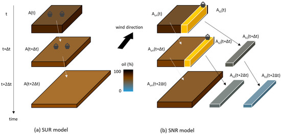
Figure 1.
Schematic drawing on the correlation between oil slick behavior and the skimming zone in (a) the spatially uniform recovery (SUR) model and (b) the spatially nonuniform recovery (SNR) model. The yellow area represents a zone where skimming is in progress. Aun: area of the unskimmed zone; As: area of the skimmed zone. The legend shows the amount of oil remaining on the sea surface, which can also be thought of as the oil thickness variation.
Furthermore, the SUR model was limited in that it considered neither the space occupied by an individual skimming system in the spatial scope of oil slick nor the interference between multiple skimming systems. Thus, when calculating the response capacity using a SUR model, the number of response resources applied to the oil slick area was virtually unlimited; the SUR model was allowed to apply the infinite quantity of skimming systems. However, there is a practical limit to the number of skimming systems that can be deployed to the limited size of an oil slick. Two spatial improvements were applied to the SNR model to overcome these two limitations.
First, to distinguish spatial differences in thickness, we differentiated the skimmed and unskimmed zones herein; Aun denotes the area of the unskimmed zone and As denotes the area of the skimmed zone. Figure 1a,b illustrate mechanisms from the SUR model and the SNR model, respectively. As shown in Figure 1a, the skimmed zone was not distinguished in the SUR model. The SNR model, however, distinguished both zones, as shown in Figure 1b. The yellow section denotes a zone in which skimming is in progress at time t. The skimming zone at time t transformed into a skimmed zone at next time, t + Δt. In other words, an area recovered by one skimming system became a skimmed zone in the next time step. The unrecovered oil among the encounter rate where the skimming system passed was regarded as the remaining oil of the skimmed zone. The amount of remaining oil in a skimmed zone equals ER minus ERR in Equation (2), by the definition of TE.
The oil thickness in the skimmed zone could be represented differently from that in the unskimmed zone because each zone was calculated separately. Furthermore, oil properties and behaviors such as weathering processes, including spreading phenomena, were calculated separately in the unskimmed and skimmed zones; it was assumed that any oil recovery during the next time step occurs only in an unskimmed zone.
Second, to consider the space occupied by an individual skimming system and interference between skimming systems, the area recovered by one skimming system and the quantity of skimming systems that can be deployed in the oil slick were computed and applied in the improved model.
Skimmers and oil booms are usually operated counter to the wind direction to take advantage of the oil movement due to wind during recovery [6]. The SNR model was thus developed to recover oil in the l2 direction. As, the area skimmed by a single skimming system in Δt, was calculated similarly to the volume rate in Equation (1), as shown in Equation (11). As the mechanical recovery was assumed to occur in the l2 direction, the l2 of the skimmed zone was identical to the l2 of the entire oil slick. The l1 length (l1s) of the skimmed zone was calculated by dividing the skimmed area As by l2:
where l1s is the l1 length of the skimmed zone. A spatial margin was added to prevent the collision of skimming systems, as shown in Equation (12). After this change, the area occupied by a single skimming system could be defined by Equation (13):
where Aoccu is the area occupied by a single skimming system and Amargin is the margin area. The full Aoccu did not represent the recovered area but was instead used to consider the interactions between skimming systems. The recovered area As is equal to Aoccu minus Amargin. l1margin is the marginal length in the l1 direction, which is assumed to be half of l1s.
Finally, the maximum number of skimming systems, x(t), that could be deployed in the unskimmed oil slick area at time t could be obtained via:
After oil recovery at time t, the l1 length of the unskimmed zone was updated via:
where l1’un(t) is the l1 length of the unskimmed zone after skimming, and l1un is the l1 length of the unskimmed zone before recovery. If there was no skimming, l1s is zero and l1’un is equal to l1un. Each space is illustrated in Figure 2.
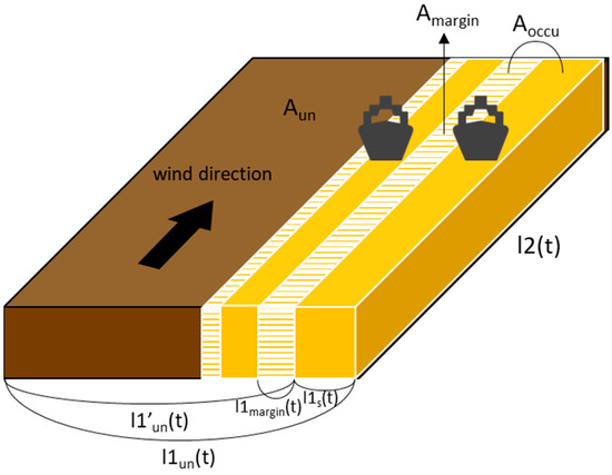
Figure 2.
Definitions of spaces used in the SNR model.
In spatially uniform recovery studies, differences in thickness due to mechanical recovery by skimming could not be resolved. The first improvement of the SNR model allowed us to distinguish skimmed and unskimmed zones, which in turn facilitates the individual calculation of the area of and oil thickness in each zone. As a result, weathering could be calculated differently for each zone, as well.
The thickness difference between the SUR model and the SNR model is illustrated in Figure 3. The SNR model supposed that encounter areas where the skimming systems passed were recovered only one time. The thickness in the SUR model tended to be slightly thinner than that of the unskimmed zone in the SNR model. A total of two zones (‘unskimmed’ and ‘skimmed‘) existed at 2 h in the SNR model because one skimming system began to recover at 1 h. The recovered zone is thinner than the unskimmed zone. This zone could be computed separately from the unskimmed zone due to the improvement mentioned below.
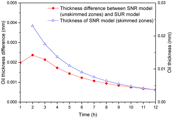
Figure 3.
Comparison between the thickness of the SNR model and SUR model; effect of distinguishing between skimmed and unskimmed zones.
The second improvement allowed the SNR model to describe the space occupancy by skimming systems and prevent interaction between them. The deployable quantity of skimming systems could also be calculated over time. In other words, the number of skimming systems that can be deployed was limited by considering interference between skimming systems. Figure 4 shows the number of skimming systems used in the calculations and the maximum number of skimming systems, x(t), that can be deployable in the unskimmed oil slick of the SNR model. In both calculations, 30 skimming systems were used as an input value. This value was applied continuously in the calculation of the SUR model. The quantity of skimming systems was 30 until 9 h in the SNR model. However, this value decreased from 10 h in the SNR model as the maximum quantity of applicable skimming systems decreased. The SNR model could consider the space occupied by an individual skimming system and the interactions between multiple skimming systems. These improvements allowed the model to reflect actual conditions better.
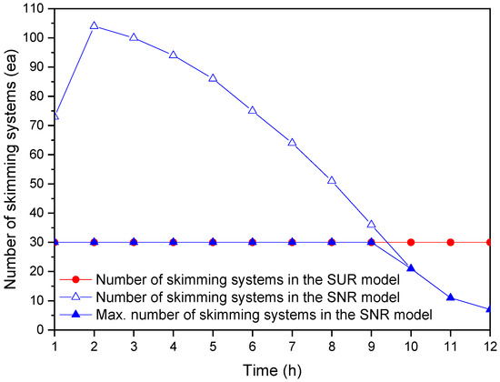
Figure 4.
Comparison of skimming systems quantity applied in the calculation and the maximum number of skimming systems, x(t), with time in the SNR model; effect of considering the space occupied by an individual skimming system and the interactions between multiple skimming systems.
2.2.2. Temporal Improvement
Oil spreading is a function of the remaining oil volume and time, and calculations of oil properties, weathering, and mechanical recovery were carried out at every time-step. The oil volume changed continuously with time due to weathering and clean-up activities, including skimming recovery. Weathering is a function of slick area (i.e., weathering may increase or decrease with the area). However, the SUR model does not explicitly reflect changes in oil volume in calculations of the spreading area, as shown in Equations (5) and (6).
The SNR model uses a remaining volume that changes continuously, instead of the initial spill volume, to reflect the changes in slick volume over time when calculating the spreading. Equations (5) and (6) in the SUR model thus have been modified to Equations (16) and (17) in the SNR model:
where V(t) is changed by weathering processes, such as oil evaporation, dispersion, and mechanical recovery.
Next, the area change over time should be calculated separately in each zone because the spatial improvement distinguished the skimmed zone and unskimmed zone. The l1 of the unskimmed zone is updated to l1’un as in Equation (15). The l1un(t + Δt) is defined by adding the increase by spreading and wind, Δl1, to the length l1’un(t):
where Δl1un(Δt) is the difference between the two l1un values calculated at time t and t + Δt in Equation (16) or Equation (17) and can be interpreted as the length increase due to spreading.
Likewise, the l1 of the skimmed zone at t + Δt could be calculated as the sum of Δl1s and the l1s(t) at the previous time step. The l1s(t) value is obtained by dividing the skimmed area As by l2 as in Equation (11), and the spreading at this value is:
The change in the length of l1 during Δt (from t to t + Δt), Δl1tot(Δt), is equal to the increase in length due to the total spreading in the unskimmed and skimmed zones:
The l2 lengths of the unskimmed and skimmed zones could be calculated using the same equation. As shown in Equation (7), l2 is defined by considering the length added due to wind to l1, which is the length considering spreading. Therefore, the spreading length Δl1 in Δt is added to the length at the previous time step. The increase in length due to wind, ΔZ, is also added:
An area comparison between the two models is shown in Figure 5. The area of the unskimmed zone, assumed to be where recovery occurred in the SNR model, is smaller than the SUR model area. Thus, the thickness of the SNR model is thicker than that of the SUR model.
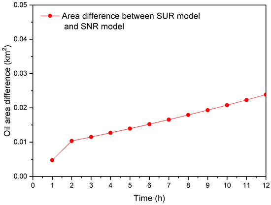
Figure 5.
Area comparison between the SUR model and the SNR model; the difference in effect reflecting thickness distribution.
Furthermore, it is possible to calculate the areas of the skimmed and unskimmed zones separately described above, using the volume of remaining oil instead of the initial spill amount. As a result, the area changes in the skimmed and unskimmed zones showed different behaviors. To separately calculate the skimmed and unskimmed zone areas, the unskimmed zone is defined as the outside the working range of the skimming systems. The spreading of the unskimmed zone during the next time step is calculated in this area. Therefore, if the skimmed area to be excluded becomes more significant than the area increment due to spreading at time t, the area of the unskimmed zone at t + Δt decreases. On the other hand, if the area increased due to spreading is larger, the area of the unskimmed zone will increase.
3. Results
3.1. Comparison of Calculation Results Using a Hypothetical Accident Scenario
In this section, the calculation results of two models (SUR model and SNR model) are compared and analyzed. The hypothetical accident scenario was created. The inputs used for the calculations are listed in Table 1. In this scenario, 500 kl of Bunker C oil was assumed to be spilled in the offshore area of Busan, Republic of Korea. The simulation time was 24 h after the accident. All 20 skimming systems were deployed from 1 h to 24 h. The three-year average wind velocity and water temperature in the Busan area [53] between 2014 and 2016 were used. Information of the Komara-50 skimmer, which is installed on the response vessel of the Busan Coast Guard, was used in the simulation. A TE was assumed to be 75%. Recovery efficiency (RE), which is defined as the percent of emulsion excluding water in the total recovered volume, was calculated over time. The size of the storage tank was assumed to be large enough to exclude time for emptying the storage tank.

Table 1.
Spill scenario of model comparison case study.
The SUR model considered reduction by both mechanical recovery and natural weathering, which includes evaporation and dispersion. The SNR model not only considered removal by recovery and weathering but also assumed that thin slicks (with a thickness of thinner than 0.6 μm) had been removed, as such slicks dissipate naturally from a response viewpoint [7,54].
As shown in Figure 6, the SNR model showed a total removal of 452 kl of oil during 24 h by three mechanisms, namely mechanical recovery, weathering, and sheen out due to thin thickness. Of this, 54% is due to recovery, 7% is due to weathering, and 39% is due to dissipation. There was no oil dissipation at 12 h. This could be explained by the thin skimmed zone generated from 17 h onward, which has a thickness of less than 0.6 μm. For example, 80 skimmed zones had a thickness of less 0.6 μm at 17 h, and the total volume of these 80 zones was approximately 29.7 kl. The total oil volume removed by dissipation during 24 h was 178 kl with 347 skimmed zones, and 20 skimmed zones were left. The same criteria were applied to the SUR model. However, no reduction in thickness to less than 0.6 μm was observed, as oil decreased over the whole oil slick body rather than in specific areas. In other words, the SUR model considered the thickness variation not by the mechanical recovery but by natural spreading. The SUR model showed a total removal of 251 kl of oil during 24 h due to two mechanisms. Of this, 230 kl was due to recovery, 21 kl was due to weathering.
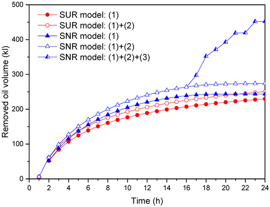
Figure 6.
Comparison of the cumulative volume of removed oil between the SUR model and the SNR model: (1) volume of oil recovered by the skimming systems, (2) volume removed by weathering, (3) volume dissipated by thin slicks with an oil thickness of less than 0.6 μm.
Figure 7 shows the number of skimming systems used in the SNR model calculation and the quantity of skimmed zones over time. Twenty skimming systems began response 1 h after the accident. Hence, 20 skimmed zones and one unskimmed zone existed at 2 h. Likewise, 20 skimmed zones appeared again due to recovery activities at 2 h, leaving 40 skimmed zones and one unskimmed zone at 3 h. In this way, the zones recovered at time t were converted to skimmed zones at t + Δt and calculated separately from the unskimmed zone. Twenty skimmed zones were newly generated at 17 h, because 20 skimming systems were operational at 16 h. At the same time, however, 80 of the existing skimmed zones dissipated due to the reduction of the thickness (i.e., <0.6 μm). Therefore, the number of skimmed zones decreased by 60 at 17 h compared to that at 16 h. The thickness of the unskimmed zone was reduced to less than 0.6 μm at 21 h. As a result, no more skimmed zones were generated. Though the applied number of skimming systems was initially constant at 20, it then dropped below 20 at 17 h, as the number of deployable skimming systems decreased with the unskimmed area (Figure 8).
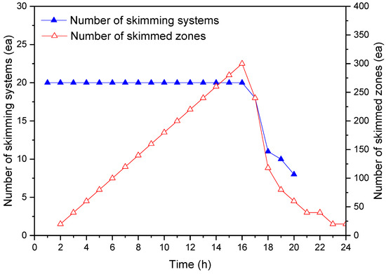
Figure 7.
The number of skimming systems used in the calculation and the number of skimmed zones with time in the SNR model.
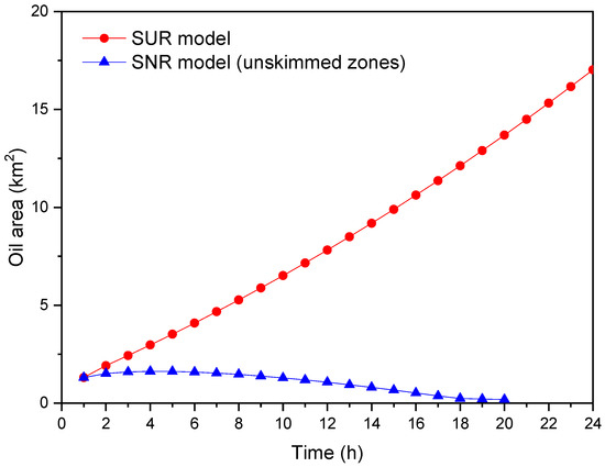
Figure 8.
Comparison between the SUR model oil slick area and the unskimmed zone area of the SNR model.
The size of the unskimmed zone (where recovery units can be operated) could be grasped in the SNR model. The SNR model took into account the space occupied by skimming systems and distinguished unskimmed and skimmed zones to consider spatial changes in thickness. Therefore, the maximum number of deployable skimming systems could also be calculated at a given time. In contrast, the SUR model did not explore the maximum number of deployable skimming systems, so 20 skimming systems were applied continuously in all calculations; spatial differences could not be distinguished, either.
Figure 8 illustrates the slick areas of the SUR model and the unskimmed zones in the SNR model. In the SUR model, the slick area was calculated as a function of the initial spill volume, as in Equations (5) and (6), and it continuously increased without reflecting the volume changes by the mechanical recovery. In contrast, it was possible to reflect volume changes since the SNR model distinguished skimmed and unskimmed zones, as described above. As the volume continuously decreased and the unskimmed zone was changed to skimmed zones beginning at 2 h by oil recovery, the unskimmed area was smaller than the SUR model area. Furthermore, area decrease could be observed in the unskimmed area from 6 h to 20 h. It was because the area converted from unskimmed to skimmed was larger than the area increases of the unskimmed zone due to spreading during this time.
The oil thickness of the unskimmed zone in the SNR model can be seen in Figure 9. In the SUR model, the volume decreased due to oil recovery in all oil slick areas. In contrast, the SNR model distinguished skimmed zones that became thin due to oil recovery from the unskimmed zone. Therefore, the thickness of the unskimmed zone was not directly affected by the mechanical removal in the SNR model. If no recovery activity was undertaken, any zone could remain unconverted into the skimmed zone. Then l1s in Equation (15) became zero, and the difference between l1 values from the SUR model and l1un from the SNR model appeared by only Equations (16) and (17). The volume reduction over time was reflected in these equations. The l1un and area in the SNR model were smaller than the l1 and area in the SUR model. The thickness of the unskimmed zone in the SNR model became thicker than that in the SUR model. However, the oil remaining in the unskimmed zone and the thickness was decreased, as mechanical recovery progressed and the unskimmed zone was converted into skimmed zones. At 21 h, the unskimmed zone dissipated as its thickness decreased below 0.6 μm, and weathering and recovery of that were no longer calculated.
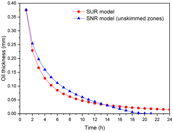
Figure 9.
Comparison of oil thickness in the SUR model and the SNR model for 24 h.
Figure 10 shows oil recovery rate and cumulative recovery volume. The recovery rate featured a trend similar to thickness, and the oil recovery rate was more significant in the SNR model than in the SUR model until 14 h. However, the recovery rate of the SNR model was lower than that of the SUR model at 15 h result from the reduced thickness in the SNR model. The amount of oil recovered during 24 h was 230 kl in the SUR model and 243 kl in the SNR model. Recovery volume of the SNR model was larger by 24 kl than that of the SUR model, despite the smaller quantity of skimming systems applied from 17 h onward.
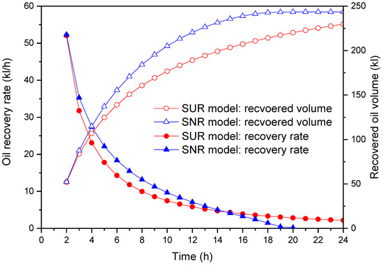
Figure 10.
Comparison of mechanical oil recovery rate and cumulative recovery volume between the SUR model and the SNR model.
The remaining oil volume on the sea surface over 24 h is illustrated in Figure 11. The total remaining volume of the SNR model was equal to the sum of unskimmed and all skimmed zones with a thickness of 0.6 μm or larger. The amount of oil remaining (compared to the initial spilled volume of 500 kl) was 50% in the SUR model and 10% in the SNR model at 24 h. However, the recovered volume of the SNR model was calculated using less than 20 skimming systems from 17 h onward. To compare the recovery time rather than volume, half of the initial spilled volume, 250 kl, is indicated in Figure 11. It took 24 h and 14 h for the volume of the remaining oil in the SUR model and the SNR model respectively to reach half of the initially spilled volume. Thus, less time was required to remove half of the initial spilled volume in the SNR model.
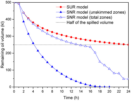
Figure 11.
Comparison of the remaining oil volume of the SUR model and unskimmed zone and total zone in the SNR model.
3.2. Comparison of Calculation Results Using Actual Accident Information
The calculation was performed using the information of the actual accident; the inputs used for the calculations are listed in Table 2. In this scenario, 900 kl of Basrah light oil was assumed to be spilled [55]. The simulation time was 72 h after the accident. Information of Normar 200TI skimmer, which was deployed on response vessel Hwangryong 208, was used in the simulation. All 10 skimming systems were applied from 1 h to 72 h. The size of the storage tank was assumed to be large enough to exclude time for emptying the storage tank.
Table 2.
Spill scenario input values using actual accident information.
The volume of remaining oil on the sea surface over 72 h is illustrated in Figure 12. The amount of oil remaining after 72 h was 390 kl in the SNR model and 494 kl in the SUR model. Recovered oil volumes were 97 kl and 109 kl for the SUR model and the SNR model, respectively. It took 140 h and 28 h, for the volume of the remaining oil in the SUR model and the SNR model respectively to reach half of the initially spilled volume.
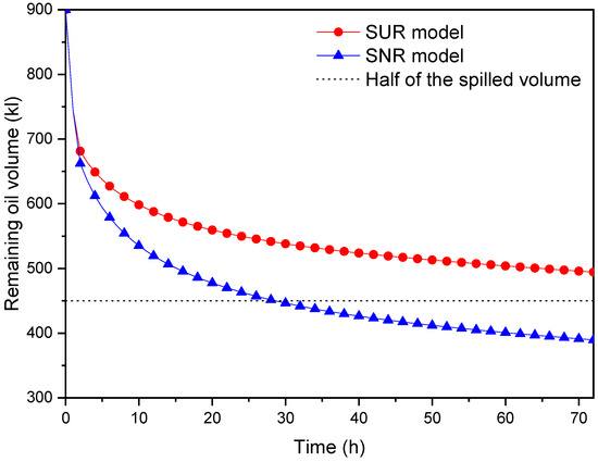
Figure 12.
Comparison of the remaining oil volume of the SUR model and the SNR model (for 900 kl spill case).
The comparisons of the number of skimming systems and recovery amounts were carried out. To remove the remaining surface oil, the SUR and SNR models required a different number of skimming systems. The comparison results among two models and response field information are summarized in Table 3. About 34 skimming systems were mobilized in the actual accident [55]. There was a significant difference between the SUR model and field data. On the other hand, the SNR model showed a similar value of field data.
Table 3.
Comparison of recovered emulsion and number of skimming systems (for 900 kl spill case).
4. Discussion
In terms of the response, various options can be employed at oil spill accidents. A skimming system can be a primary choice among mechanical recovery, chemical dispersion, and in situ burning. Numerous studies have been conducted to forecast spilled oil behaviors and establish response strategies for oil spill accidents at sea. However, current research remains insufficient on recovery potential estimation methods that consider oil weathering, slick behavior, and equipment efficiency. Many previous studies that aim to maximize the recovery focused on the window-of-opportunity [6,7,31,32,33,34,35,36,37], the performance of skimmers [38,39,40], and clean-up potential [32,41,42]. Nevertheless, it is still required to study the response in terms of recovery capacity. The mechanical recovery potential estimation model of the present study can help decision-makers to set up the mobilization and deployment plan of the skimming systems. It is beneficial to estimate the potential of mechanical recovery systems in terms of recovery capacity in the response-planning phase. The present study is not designed to command the field response activities but to support the expert group by providing the response planning tool.
Two models were developed in this study. One is the SUR model that does not consider skimmed zone and local thickness variations, and the other is a model considering skimmed zone and thickness distribution (the SNR model). Three improvements that allow the model to reflect more specific conditions were implemented in the SNR model. The calculation of two models was conducted through the hypothetical and actual accident scenarios to compare the effects of the spatial and temporal improvements.
The calculation of the hypothetical accident case study revealed that the total recovered oil volume was 230 kl in the SUR model and 243 kl in the SNR model for 24 h. There was little difference between the SUR and SNR models in the oil recovery rate and volume from Figure 10. On the other hand, the remaining oil volume in the sea surface showed a considerable difference between the two models in Figure 11. Furthermore, it took 24 h and 14 h for the volume of remaining oil in the SUR and SNR models, respectively, to reach half of the initially spilled volume. Thus, less time was required to remove half of the initially spilled volume in the SNR model. It seems that the improvement of the SNR model well facilitates the sheen out of the remaining thin oil in the skimmed zones. Moreover, the actual accident case study showed a significant difference in calculation results. The SNR model calculated a similar number of skimming systems and recovery amounts with the field data.
Nevertheless, it is better to clarify the limitation of the SNR model. Skimming systems do not work like vacuum cleaners in actual spills. It means that the field operation of the skimming systems cannot precisely follow the mathematical model of the present study. The SUR and SNR models can mathematically calculate any size of the spill and recovery. However, that does not mean that both models can be applied to any size and shape of the slick. The spreading of oil is a very complicated process. The present study used the spreading models of Fay [51] and Galt and Overstreet [47] in calculating the slick area. Therefore, the uncertainty of the present study is the same as that of the previous models.
To identify the uncertainty of the SNR model, the effect of the parameter on the calculation results was analyzed. Mathematical modeling of the SNR model was developed to distinguish spatial differences in thickness between the skimmed and unskimmed zones. In addition, a spatial margin was added to prevent the collision of skimming systems, as shown in Equation (12). This marginal length might make some uncertainty on the number of skimming systems during the calculation. The uncertainty due to this marginal length was quantitatively analyzed for the 500 kl spill case study of Section 3.1. In the normal condition, the marginal length in the l1 direction, l1margin, is assumed to be half of l1s. The uncertainty of the calculation results was analyzed by varying the marginal length from the half to the double of the normal size condition. The number of skimming systems were compared in Figure 13. As the marginal length increased, the recovery time when a total of 20 skimming systems were operated decreased. Figure 14 shows the number of skimmed zones. The smaller the marginal length, the more the skimmed zones. The remaining oil volume of uncertainty study is summarized in Table 4.
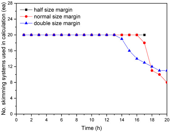
Figure 13.
Effect of marginal length on the number of skimming systems (uncertainty of SNR model for 500 kl spill case study).
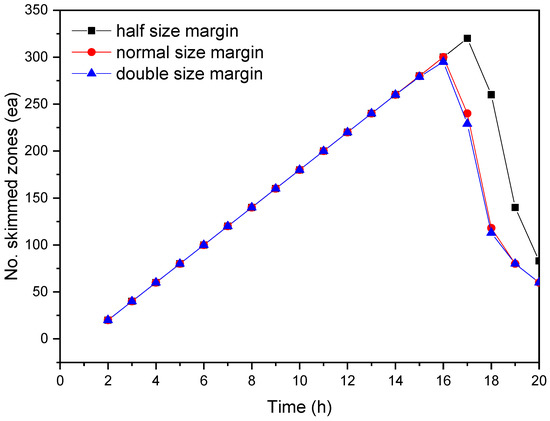
Figure 14.
Effect of marginal length on the number of skimmed zones (uncertainty of SNR model for 500 kl spill case study).
Table 4.
Effect of marginal length on the remaining oil volume of unskimmed zones (uncertainty of SNR model for 500 kl spill case study).
Unfortunately, the skimming systems cannot entirely cover a wide geographic area in the case of very large-scale catastrophic spill accidents. It is essential to be guided with aerial observation and remote sensing. The deployment of the skimming systems could be directed to the thickest oil with aerial support to optimize recovery. The approach of the present study can be used to start with one slick and then tracks portions of it as skimming varies spatially and over time. That said, it is practically difficult to handle all the slicks in the same manner with the present model. Most numerical oil spill models are based on a Lagrangian approach. The Lagrangian spill model, aerial observation, and remote sensing could give the present recovery model the information on the location and thickness of slick. Then, the present recovery model can be used to estimate the mechanical recovery potential based on the collected information, but there are many technical challenges to handle this issue. It will be future work.
Finally, even though the SNR model cannot perfectly reflect all details of field conditions, it can allow a better understanding of the effect of nonuniformity in recovery activities on the response effectiveness and the amount of oil remaining floating. It will be helpful to make a response plan. Given enough accident information, this model can be utilized to estimate and reserve the necessary response resources in the event of oil spill accidents.
5. Conclusions
The recovery capacity of the mechanical skimming systems should be carefully considered in the response-planning phase. To make a suitable response strategy, it is necessary to assess mechanical recovery capacity. The SNR and SUR models of the present study consisted of weathering calculation and recovery calculation. The recovery calculation made a change in sea surface oil volume, and then the volume change made an effect in weathering calculation, and vice versa. To evaluate the spatial and temporal improvement of the SNR model, the recovery potential and its effects on the responses were compared and analyzed using case studies. The main findings are described below.
First, spatially uniform studies are limited in that the whole remaining oil in the sea surface is considered a single oil slick, with no spatial variations in thickness by mechanical clean-up activities. The first improvement in the SNR model considers these spatial changes in thickness by distinguishing areas where oil recovery was performed from those where it was not. Through this change, a more realistic mechanical recovery volume can be calculated using the thickness of each zone; the area of and weathering in each zone can also be calculated separately. This zone distinction in the SNR model allowed the model to represent thin slicks, which could not be easily distinguished in the SUR model, and reflect natural oil dissipation effects by clean-up activities. In the calculation result through the SNR model, a total of 367 skimmed zones were distinguished. In all, 347 zones of total skimmed zones and the unskimmed zone with thin thickness dissipated during 24 h, leaving 20 skimmed zones at 24 h in the case study.
Second, the SUR model takes into account neither the space occupancy by a skimming system nor spatial inference with other skimming systems. Therefore, any quantity of skimming systems could be deployed by the user during the calculations with no spatial constraints. That leads to an unaffordable response strategy in decision-making. The second improvement of the SNR model involved the calculation of both the space occupied by a skimming system and the interactions between skimming systems. This allowed the improved model to estimate the maximum applicable number of skimming systems over time and use this number in the recovery potential calculation. The unskimmed area in the SNR model decreased over time. As a result, the quantity of deployable skimming systems also decreased, and this decrease was reflected in the recovery volume calculation. The upper limit to the number of skimming systems depends on the slick area, and thus the number of skimming systems applied in the calculation changes with time. This enables the application of more realistic quantities of available skimming systems in the model. It will be very helpful in recovery strategy decision-making.
Third, spatially uniform studies calculate oil spreading using the initial spill volume, and changes in the residual oil volume due to weathering processes (such as evaporation and natural dissipation) and mechanical recovery were not considered. That can be a critical limitation in accessing the remaining oil mass balance, as the oil volume and area are essential factors in recovery potential calculations. The third improvement applied in the SNR model made it possible to consider the residual oil volume changes at the sea surface with time.
Author Contributions
Conceptualization, C.H.; methodology, Y.C., H.K. and C.H.; investigation and analysis, Y.C., H.K. and C.H.; writing—review and editing, Y.C. and C.H.; funding acquisition, C.-K.K., M.-I.C. and H.-J.C. All authors have read and agreed to the published version of the manuscript.
Funding
This research was a part of the project titled ‘Marine Oil Spill Risk Assessment and Development of Response Support System through Big Data Analysis’, funded by the Korea Coast Guard, grant number KCG-01-2017-05, ‘Development of mathematical modeling technology for CO2-CH4 multi-fluid subsea transport’, funded by the National Research Foundation of Korea (NRF), grant number 2017R1E1A1A03070672 and ‘Amphibious Recovery Technology and Equipment Development of Large Scale Marine Inflow Oil’, funded by the Korea Coast Guard, grant number 20190483.
Conflicts of Interest
The authors declare no conflict of interest.
References
- IEA. Oil 2019 Executive Summary; Analysis and Forecast to 2024; IEA: Paris, France, 2019. [Google Scholar]
- BP. BP Statistical Review of World Energy 2019; BP: London, UK, 2019. [Google Scholar]
- Musk, S. Trends in oil spills from tankers and ITOPF non-tanker attended incidents. In Proceedings of the Thirty-fifth AMOP Technical Seminar on Environmental Contamination and Response. Environment Canada, Vancouver, BC, Canada, 5–7 June 2012; pp. 775–797. [Google Scholar]
- ITOPF. Oil Tanker Spill Statistics 2018. Available online: https://www.itopf.org/knowledge-resources/data-statistics/statistics/ (accessed on 23 October 2019).
- Chen, J.; Zhang, W.; Wan, Z.; Li, S.; Huang, T.; Fei, Y. Oil spills from global tankers: Status review and future governance. J. Clean. Prod. 2019, 227, 20–32. [Google Scholar] [CrossRef]
- Fingas, M. Oil Spill Science and Technology, 1st ed.; Gulf Professional Publishing: Houston, TX, USA, 2010; ISBN 978-1-85617-943-0. [Google Scholar]
- Fingas, M. Oil Spill Science and Technology, 2nd ed.; Gulf Professional Publishing: Houston, TX, USA, 2016; ISBN 978-0-12-809413-6. [Google Scholar]
- Fingas, M.; Brown, C.E. A review of oil spill remote sensing. Sensors 2018, 18, 91. [Google Scholar] [CrossRef] [PubMed]
- Kim, H.; Choe, Y.; Huh, C. Estimation of a Mechanical Recovery System’s Oil Recovery Capacity by Considering Boom Loss. J. Mar. Sci. Eng. 2019, 7, 458. [Google Scholar] [CrossRef]
- Mooney, M. The viscosity of a concentrated suspension of spherical particles. J. Colloid Sci. 1951, 6, 162–170. [Google Scholar] [CrossRef]
- Jokuty, P.; Fingas, M.; Whiticar, S.; Fieldhouse, B. A Study of Viscosity and Interfacial Tension of Oils and Emulsions; Environmental Protection Service, Environment Canada: Ottawa, ON, Canada, 1995.
- Song, B.; Springer, J. Determination of interfacial tension from the profile of a pendant drop using computer-aided image processing: 1. Theoretical. J. Colloid Interface Sci. 1996, 184, 64–76. [Google Scholar]
- Fingas, M.; Fieldhouse, B. Studies on crude oil and petroleum product emulsions: Water resolution and rheology. Colloids Surf. A Physicochem. Eng. Asp. 2009, 333, 67–81. [Google Scholar] [CrossRef]
- Fingas, M.; Fieldhouse, B. Studies on water-in-oil products from crude oils and petroleum products. Mar. Pollut. Bull. 2012, 64, 272–283. [Google Scholar] [CrossRef] [PubMed]
- Monahan, E.C. Oceanic Whitecaps. J. Phys. Oceanogr. 1971, 1, 139–144. [Google Scholar] [CrossRef]
- Mackay, D.; Matsugu, R.S. Evaporation rates of liquid hydrocarbon spills on land and water. Can. J. Chem. Eng. 1973, 51, 434–439. [Google Scholar] [CrossRef]
- Payne, J.R.; Kirstein, B.E.; McNabb, G.D., Jr.; Lambach, J.L.; de Oliveira, C.; Jordan, R.E.; Hom, W. Multivariate Analysis of Petroleum Hydrocarbon Weathering in the Subarctic Marine Environment; American Petroleum Institute: Washington, DC, USA, 1983; Volume 1983, pp. 423–434. [Google Scholar]
- Payne, J.; Kirstein, B.; McNabb, G.D., Jr.; Lambach, J.; Redding, R.; Jordan, R.; Hom, W.; De Oliveira, C.; Smith, G.; Baxter, D. Multivariate Analysis of Petroleum Weathering in the Marine Environment–Sub Arctic; US Department of Commerce, National Oceanic and Atomospheric Administration: AK, USA, 1984.
- Delvigne, G.A.L.; Sweeney, C. Natural dispersion of oil. Oil Chem. Pollut. 1988, 4, 281–310. [Google Scholar] [CrossRef]
- Eley, D.; Hey, M.; Symonds, J. Emulsions of water in asphaltene-containing oils 1. Droplet size distribution and emulsification rates. Colloids Surf. 1988, 32, 87–101. [Google Scholar] [CrossRef]
- Zeinstra-Helfrich, M.; Koops, W.; Murk, A.J. The NET effect of dispersants—A critical review of testing and modelling of surface oil dispersion. Mar. Pollut. Bull. 2015, 100, 102–111. [Google Scholar] [CrossRef] [PubMed]
- Spaulding, M.L. A state-of-the-art review of oil spill trajectory and fate modeling. Oil Chem. Pollut. 1988, 4, 39–55. [Google Scholar] [CrossRef]
- Sebastiao, P.; Soares, C.G. Modeling the fate of oil spills at sea. Spill Sci. Technol. Bull. 1995, 2, 121–131. [Google Scholar] [CrossRef]
- Reed, M.; Johansen, Ø.; Brandvik, P.J.; Daling, P.; Lewis, A.; Fiocco, R.; Mackay, D.; Prentki, R. Oil spill modeling towards the close of the 20th century: Overview of the state of the art. Spill Sci. Technol. Bull. 1999, 5, 3–16. [Google Scholar] [CrossRef]
- Mackay, D.; Shiu, W.Y.; Hossain, K.; Stiver, W.; McCurdy, D. Development and Calibration of an Oil Spill Behavior Model; Toronto Univ (Ontario) Dept of Chemical Engineering and Applied Chemistry: Toronto, ON, Canada, 1982. [Google Scholar]
- Berry, A.; Dabrowski, T.; Lyons, K. The oil spill model OILTRANS and its application to the Celtic Sea. Mar. Pollut. Bull. 2012, 64, 2489–2501. [Google Scholar] [CrossRef]
- Guard, U.C. On Scene Coordinator Report Deepwater Horizon Oil Spill: Submitted to the National Response Team, September 2011; United States Coast Guard: Washington, DC, USA, 2011; p. 2014. [Google Scholar]
- Kerr, R.A. A Lot of Oil on the Loose, Not So Much to Be Found. Science 2010, 329, 734–735. [Google Scholar] [CrossRef]
- Lehr, B.; Nristol, S.; Possolo, A. Oil Budget Calculator—Deepwater Horizon, Technical Documentation: A Report to the National Incident Command; The Federal Interagency Solutions Group: USA, 2010. [Google Scholar]
- Conrad, J.M. Oil spills: The strategy of recovery. Coast. Zone Manag. J. 1978, 4, 409–434. [Google Scholar] [CrossRef]
- Nordvik, A.B. The technology windows-of-opportunity for marine oil spill response as related to oil weathering and operations. Spill Sci. Technol. Bull. 1995, 2, 17–46. [Google Scholar] [CrossRef]
- Nordvik, A.B. Time window-of-opportunity strategies for oil spill planning and response. Pure Appl. Chem. 1999, 71, 5–16. [Google Scholar] [CrossRef][Green Version]
- Bjerkemo, O.K. Behaviour of Oil and HNS Spilled in Arctic Waters–an Arctic Council Project; American Petroleum Institute: Washington, DC, USA, 2011; Volume 2011, p. abs229. [Google Scholar]
- Zhang, C.; Nedwed, T.; Tidwell, A.; Urbanski, N.; Cooper, D.; Buist, I.; Belore, R. One-Step Offshore Oil Skim and Burn System for use with Vessels of Opportunity; American Petroleum Institute: Washington, DC, USA, 2014; Volume 2014, pp. 1834–1845. [Google Scholar]
- Nedwed, T. Recent Advances in Oil Spill Response Technologies; European Association of Geoscientists & Engineers: Houten, The Netherlands, 2013; p. cp-350. [Google Scholar]
- Westerberg, V. Arctic Oil Spill Response: Recovery operations-Management and Performance; SSPA: Sweden, 2012. [Google Scholar]
- Champ, M.A.; Nordvik, A.B.; Simmons, J.L. Utilization of Technology Windows of Opportunity in Marine Oil Spill Contingency Planning, Response, and Training; American Petroleum Institute: Washington, DC, USA, 1997; Volume 1997, pp. 993–994. [Google Scholar]
- Schultz, R. Oil Spill Response Performance Review of Skimmers; ASTM Manual Series; ASTM: West Conshohocken, PA, USA, 1998; ISBN 978-0-8031-2078-5. [Google Scholar]
- ASTM. ASTM F631–15-Standard Guide for Collecting Skimmer Performance Data in Controlled Environments; ASTM: West Conshohocken, PA, USA, 2015. [Google Scholar]
- ASTM. ASTM F1780-18 Standard Guide for Estimating Oil Spill Recovery System Effectiveness; ASTM: West Conshohocken, PA, USA, 2018. [Google Scholar]
- Lehr, W.J. Review of modeling procedures for oil spill weathering behavior. Adv. Ecol. Sci. 2001, 9, 51–90. [Google Scholar]
- Oebius, H.U. Physical properties and processes that influence the clean up of oil spills in the marine environment. Spill Sci. Technol. Bull. 1999, 5, 177–289. [Google Scholar] [CrossRef]
- Allen, A.; Dale, D.; Galt, J.; Murphy, J. Effective Daily Recovery Capacity (EDRC) Project Final Report; Genwest System and Spiltec: Edmonds, WA, USA, 2012. [Google Scholar]
- BSEE. ERSP Calculator User Manual 2015; Genwest Systems, Inc.: Edmonds, WA, USA, 2015. [Google Scholar]
- Casey, D.; Caplis, J. Improving Planning Standards for the Mechanical Recovery of Oil Spills on Water; American Petroleum Institute: Washington, DC, USA, 2014; Volume 2014, pp. 1772–1783. [Google Scholar]
- Dale, D. Response Options Calculator (ROC) Users Guide; Genwest Systems, Inc.: Edmonds, WA, USA, 2011. [Google Scholar]
- Galt, J.; Overstreet, R. Development of Spreading Algorithms for the ROC; Genwest Systems, Inc.: Edmonds, WA, USA, 2009. [Google Scholar]
- Dale, D. Response Option Calculator (ROC) Technical Documentation; Genwest Systems, Inc.: Edmonds, WA, USA, 2011. [Google Scholar]
- Galt, J.A. Oil Weathering Technical Documentation and Recommended Use Strategies. Available online: https://www.genwest.com/wp-content/uploads/2017/09/Oil-Weathering-Tech-Doc-Recommeded-Use-Strategies.pdf (accessed on 21 May 2020).
- Ermakov, S.A.; Danilicheva, O.A.; Kapustin, I.A.; Molkov, A.A. Drift and Shape of Oil Slicks on the Water Surface; International Society for Optics and Photonics: Bellingham, WA, USA, 2019; Volume 11150, p. 111500J. [Google Scholar]
- Fay, J.A. The spread of oil slicks on a calm sea. In Oil on the Sea; Springer: Berlin/Heidelberg, Germany, 1969; pp. 53–63. [Google Scholar]
- Kinsman, B. Wind Waves: Their Generation and Propagation on the Ocean Surface; Courier Corporation: North Chelmsford, MA, USA, 1984; ISBN 0-486-64652-1. [Google Scholar]
- Korea Hydrographic and Oceanographic Agency Oceanographic Observation Portal. Available online: http://www.khoa.go.kr/kcom/cnt/selectContentsPage.do?cntId=31000000 (accessed on 24 September 2019).
- ITOPF. Aerial Observation of Marine Oil Spills; ITOPF Technical Information Paper; ITOPF: London, UK, 2011. [Google Scholar]
- Korea Coast Guard. Oil Spill Response Report; Korea Coast Guard: Incheon, Korea, 2015; pp. 105–121. [Google Scholar]
© 2020 by the authors. Licensee MDPI, Basel, Switzerland. This article is an open access article distributed under the terms and conditions of the Creative Commons Attribution (CC BY) license (http://creativecommons.org/licenses/by/4.0/).