Developing a Pilot Operational Oceanography System for an Enclosed Basin

Abstract

The first stages of the development of a pilot oceanographic observatory for an enclosed basin (Kalloni Gulf, Lesvos, Greece) are described. The focus of the present work is related to the estimation of the water exchange with the open sea, using a numerical model of the region, volume flux measurements based on current velocity, and sea-level measurements. Three different methods of assessment of the exchange are described and evaluated, in order to select a reference method to calibrate submarine telephone cable measurements. The high-resolution coastal circulation model for the enclosed sea, nested in a larger-domain model, is developed and evaluated against in situ data, focusing on the adequate representation of the exchange and the hydrographic structure in the basin. Monitoring the water level is selected as the best-suited method for estimating the water exchange in hourly-to-weekly time scales. The model reproduces adequately the tidal exchange and sea-level response, as well as the hydrographic characteristics of the basin. The cable voltage measurements exhibit tidal signals overwhelmed by low-frequency noise, possibly attributable to circuitry and ground failures; however, the most suitable method for estimating exchanges of the basin with the open sea appears to be sea-level monitoring.

1. Introduction

Enclosed and semi-enclosed coastal marine basins constitute areas of specific oceanographic interest due to their role as sources of anomalous property waters for the open sea, as well as their socioeconomic significance [1]. The contribution of land effluents and coastal microclimate, as well as relatively shallow water depths and small volumes, often cause the waters of such coastal areas to obtain hydrographic and ecosystem characteristics significantly different from those of the neighboring (and interacting) open sea. These regions exchange water with the offshore areas through the connecting straits, and function as sources of diversified water for the open sea, which in turn may affect the latter’s circulation and hydrographic properties. For that reason, special attention is directed to the suitable representation of these basins in general circulation models of regional scale, lacking the appropriate resolution to adequately reproduce the thermohaline functioning of the enclosed basins and their exchanges with the open sea [2,3,4].

In addition to the role that these basins play in the circulation and hydrography of the neighboring open sea, the specific hydrographic and biogeochemical characteristics of these basins greatly enhance their ecological and socioeconomic importance [5]. Due to their limited geographical area and the concentration of human population and activities there, enclosed basins exhibit a much higher sensitivity to human impacts [6] and thus there is a pressing need for drafting comprehensive and effective management policies, especially due to the range of contrasting pressures and demands from the different coastal stakeholder groups. However, the aim of drafting management policies for a coastal region requires exceptionally good understanding of the natural and anthropogenic processes and their ecological and socioeconomic impacts, and the associated development of monitoring and forecasting tools e.g., [7].

Currently, a great deal of effort is invested in developing, maintaining, expanding and managing operational oceanographic monitoring and forecasting, as well as database networks and providing services to a wide range of users [8,9]. These efforts are concentrated at global or regional scales, whose spatiotemporal coverage is essential in monitoring, understanding and responding to global-scale anthropogenic changes. However, due to the ecological and socioeconomic importance of coastal processes, similar networks dedicated to coastal monitoring have been formed and are under continuous development and expansion [10]. The Department of Marine Sciences of the University of the Aegean, aiming to develop a prototype oceanographic monitoring and forecasting observatory to support Blue Growth investment at local and regional scale, has selected the Gulf of Kalloni, of Lesvos Island, Greece, for a pilot application.

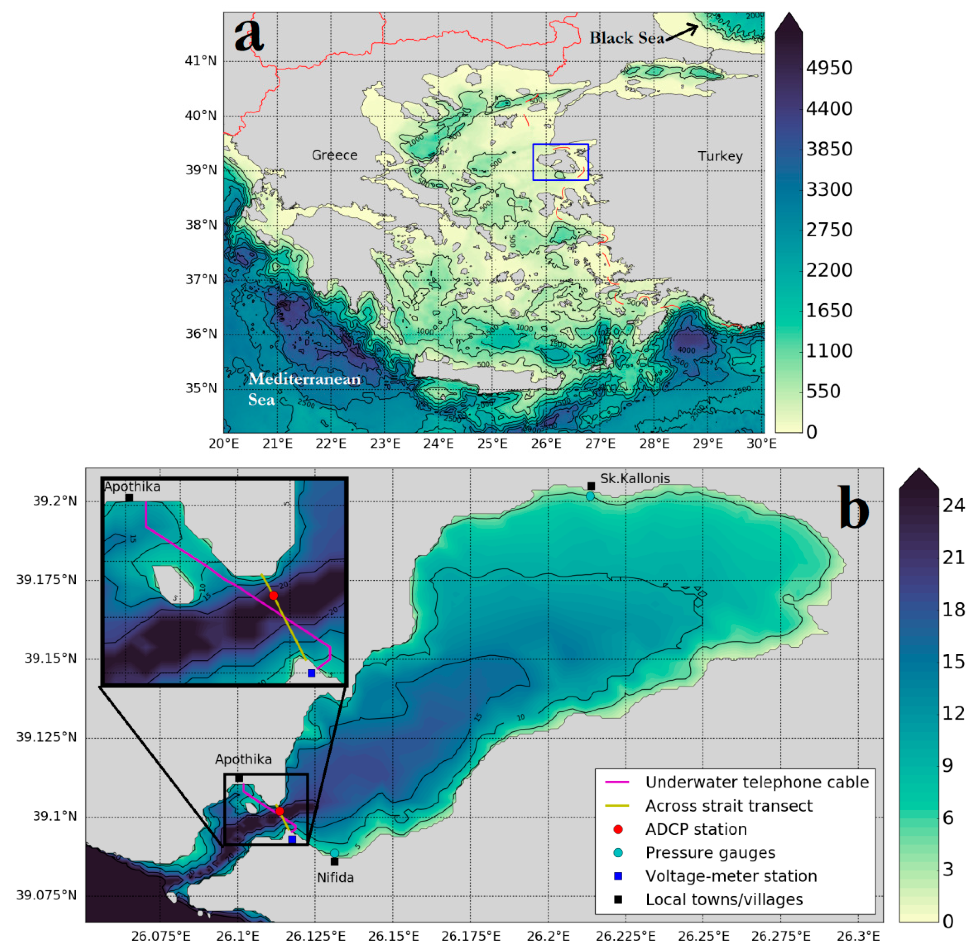
Area of Study: The Gulf of Kalloni

Kalloni Gulf is located at the center of Lesvos, an island of the north-eastern Aegean Sea (Figure 1), and is the one of the most productive and diverse coastal regions of the Eastern Mediterranean [11,12,13]. The wealth of its coastal ecosystem triggered Aristotle’s interest in describing organisms, their behavior and relationships, thus setting the basis of what is now called biology [14]. The gulf attracts various coastal activities, with significant anthropogenic impacts [15,16,17,18], so that a comprehensive management policy needs to be devised. This policy, however, is still in its early stages [19].

The Kalloni Gulf was formed by the flooding of the mountainous paleo-valley during the most recent glacial-interglacial transition. Thus, its bottom topography is not typical of enclosed or semi-enclosed basins: the strait connecting the gulf with the open sea lacks a sill separating the deep layers of the two basins, so that the exchange is controlled by the width and not the depth of the strait. This characteristic is typical of the gulfs of the Aegean islands, and thus developing a monitoring and forecasting system for the Kalloni Gulf may lead the way to develop a pilot management system for a number of coastal regions in Greece and abroad.

Other reasons for selecting the Kalloni Gulf for developing a pilot Coastal Observatory include:

(1)

The presence of a submerged telephone cable crossing the strait, potentially enabling us to obtain long-term, high-frequency estimates of the net exchange with the open sea [20,21] at minimal cost.

(2)

The ecological and socioeconomic significance of the gulf, which calls for the development of monitoring and forecasting infrastructure.

(3)

The vicinity of the gulf to the premises of the Department of Marine Sciences of the University of the Aegean, which would limit logistical costs and enable the exploitation of the Observatory for not only research, but also educational activities.

The present work constitutes the first step towards the development of the Coastal Observatory. The aim is to develop a pre-operational coastal monitoring and simulation system that will be able to adequately describe the exchange with the open ocean and the temporal evolution of the hydrographic characteristics of the gulf, in order to provide the basis for further development of a forecasting tool, a climatic projection tool and an ecosystem model for the region.

The development of the above-described pre-operational system requires the development of a coastal circulation model, as well as an observational strategy that will enable us to assess the model’s performance. In this work, emphasis is given on the development and application of several different methods to assess the net exchange at the strait, in order to provide a basis for calibration of the submarine telephone cable method, as well as validate the numerically-simulated exchanges.

An important factor for better understanding the physical characteristics of the basin, and one that must be addressed and quantified in this study, is the net water volume exchange at the connecting strait. In this framework, testing of different methods that can be used for this purpose is also of major importance. The cable method’s applicability, although having been exploited in several studies, is not yet certain in assessing the net exchange in this case for different reasons. First, a stable calibration curve to enable the accurate description of the net flux needs to be developed. In addition, the submarine cable’s route differs significantly from a simple cross-section of the strait (see Figure 1b,c), so the cable-estimated fluxes could differ from the fluxes through the strait. The numerical modelling method needs to be validated based on its accuracy in describing the exchange flow and reproducing the hydrographic properties of the gulf’s waters.

In the following section (“Materials and Methods”), three different methods are described for the assessment of the net exchange flow at the strait, to serve as reference for calibration of the cable measurements. In the same section, a brief description of the modelling strategy and implementation is given. The results of our data analyses, simulations and their comparison are described in the next section, to be followed by the discussion and conclusions sections.

2. Materials and Methods

2.1. Observational component—Exchanges at the Strait

The observation component of the Kalloni oceanographic system addressed herein focuses mainly on quantifying the volume exchange with the Aegean Sea in order to provide a basis of evaluation for the numerical model, as well as reference values for calibration of the submarine telephone cable method.

The assessment of the net exchange through the strait is based on estimating the terms of the water volume budget of the basin:

$$\frac{dV}{dt}=Q_{net}+P+R-E,$$

(1)

where $V$ is the volume of the basin, $Q_{net}$ the net water volume flux rate exchanged with the open sea through the strait (where positive values denote net inflow to the basin), $P$ the precipitation rate, $R$ the land effluents’ rate and $E$ the evaporation rate over the basin.

Over the time scale of a few days, and especially during the dry summer, when both precipitation and riverine input are approximately zero and the evaporation is of the order of a few mm per day, the atmospheric terms of Equation (1) can be neglected, since (as will be shown below, the variability of the sea-level is of the order of several cm, dominated by tides, while atmospheric and land mass exchanges amount to rates of the order of mm over several hours). Then, the rate of change of the basin volume is controlled by the net exchange at the straits:

$$\frac{dV}{dt}\simeq Q_{net}.$$

(2)

The submarine telephone cable provides us with a means to measure the voltage between the two shores across the strait and convert that to $Q_{net}$ measurements, assuming a net volume flux versus voltage curve is constructed to be used as the calibration curve.

In order to construct the calibration curve, two methods have been used to directly estimate net volume flux $Q_{net}$, and one to estimate it indirectly by measuring the rate of change of the water volume in the basin and using Equation (2) to obtain $Q_{net}$.

2.1.1. Submarine Telephone Cable Method

This method aims to record the electrical voltage difference between the two coasts of a strait, using the submarine cable as an extension of one of the electrodes of a voltmeter located on one coast to reach the opposite coast (Figure 1). In the Gulf of Kalloni case, the cable is an active optical fiber cable, and a metal shield has been used to carry the signal of the voltage potential from one coast to the other. The instrumentation, consisting of a FLUKE 8846A laboratory voltmeter connected to a Raspberry Pi micro PC acting as a data logger, was installed on the beach of Nyfida, next to the landing site of the submarine cable. One electrode of the voltmeter was locally grounded, and the other was connected to the shield of the submarine optical fiber cable, grounded on the Apotheka coast across the strait. The cable provided a cross-strait voltage time-series, extending from 2019-06-19 15:00 UTC to 2019-07-03 09:00 UTC, sampled every 1 second and averaged over 5-min intervals.

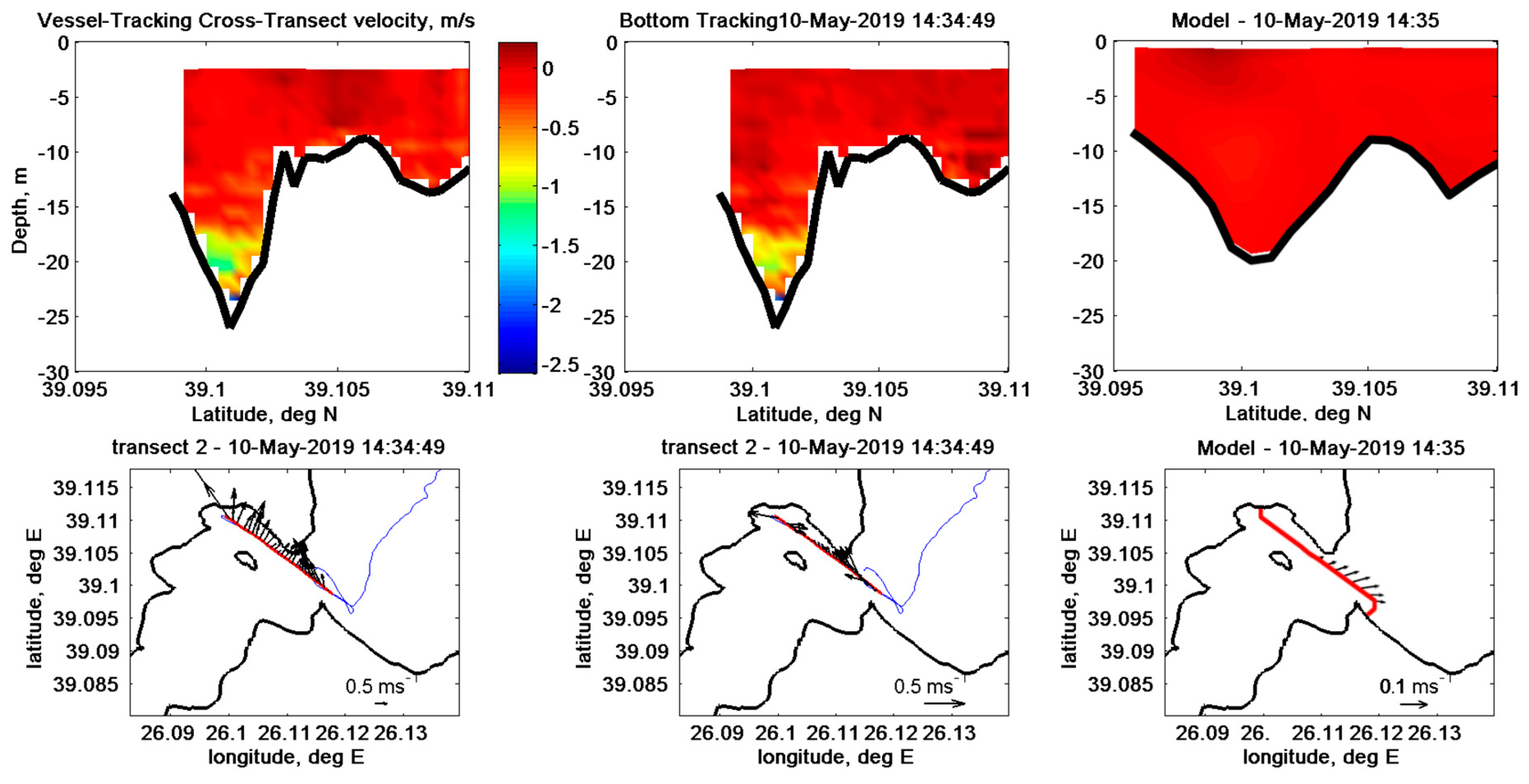
2.1.2. Volume Flux via Shipborne Acoustic Doppler Current Profiler Transects

A Nortek AWAC Acoustic Doppler Current Profiler transmitting at 600 kHz was attached off the port side of coastal research vessel R/V “Amphitriti” with the transmitters facing downwards. Two routes were followed by the vessel between the two coasts: one route directly followed the submarine cable path, from Nyfida beach to the village of Apotheka (hereafter referred to as the “long” route), and the other route was from Cape Perama (on the southern coast) to Cape Lena (on the northern coast), hereafter identified as the “short” route. The short route, of length about 0.5 km, corresponds approximately to part of the long route, of approximate length 2.5 km.

Table 1. List of transects performed across the strait.

Month	Date	Start Time (UTC)	End Time (UTC)	Sampling Interval (s)	Transect Type
May	9/5/2019	18:10	18:13	30	Long
	10/5/2019	11:27	11:33	30	Short
	10/5/2019	11:27	11:42	30	Long
	10/5/2019	11:42	11:57	30	Long
	10/5/2019	11:51	11:57	30	Short
	11/5/2019	13:49	13:55	10	Short
	11/5/2019	13:49	14:07	10	Long
	11/5/2019	14:08	14:26	10	Long
	11/5/2019	14:19	14:26	10	Short
	11/5/2019	14:29	14:40	10	Long
	11/5/2019	14:34	14:40	10	Short
	11/5/2019	14:40	14:46	10	Short
	12/5/2019	07:35	07:51	10	Long
	12/5/2019	07:35	07:41	10	Short
	12/5/2019	07:50	08:06	10	Long
	12/5/2019	08:00	08:06	10	Short
	12/5/2019	08:12	08:17	10	Short
	12/5/2019	08:17	08:22	10	Short
June	12/6/2019	10:31	10:38	10	Short
	12/6/2019	10:38	10:45	10	Short
	12/6/2019	10:45	10:52	10	Short
	12/6/2019	10:52	10:59	10	Short
	12/6/2019	11:00	11:96	10	Short
	19/6/2019	10:26	10:33	10	Short
	21/6/2019	13:51	13:56	10	Short
	24/6/2019	15:17	15:24	10	Long
	24/6/2019	15:24	15:30	10	Long
	24/6/2019	15:24	15:30	10	Long

presents the transects performed from May to June 2019 in an effort to collect as many volume flux estimates as possible.

The Nortek AWAC used in this study is not equipped with an inherent bottom tracking capability. Thus, two different methods were used to obtain absolute velocity profiles from the velocity relative to the AWAC’s transducers as recorded and provided by the instrument. The first method was a bottom-tracking technique, removing the AWAC-measured velocity of the most reflective depth-bin, corresponding to the seabed. The second method, referred to hereafter as the vessel-tracking technique, consisted of removing the vessel’s velocity as provided by the shipborne GPS. Results from applying both methods on a transect, as well as the modelled results, are presented in Figure 2. Based on the analysis presented in Section 3.2, the deep undercurrent appearing below ~17m in the observed transects is attributed to instrumental noise.

In order to obtain volume flux from the transect velocity data, the cross-transect velocity component was integrated vertically and horizontally along the vessel’s path:

$$Q_{net}={{\displaystyle \int }}_{L_1}^{L_2}{{\displaystyle \int }}_{-H\left(x\right)}^{0}u\left(x,z\right)dzdx,$$

(3)

where x is the along-transect horizontal coordinate, z the vertical coordinate, u the cross-transect velocity component, H(x) the water-depth a location x along the transect, and L₁, L₂ the beginning and end of the transect, respectively. As the boat did not reach the coast at any transect, the flow from the coast (or the seabed) to the nearest velocity measurements was assumed to be equal to the mean flow for each depth bin.

2.1.3. Volume Flux via Moored Acoustic Doppler Current Profiler (ADCP) Method

The volume flux through the strait was also estimated for a short period of time, from 2019-06-16 07:05 UTC to 2019-06-21 17:15 UTC using a Nortek Continental ADCP transmitting at 1000 kHz, deployed in an upward-looking mode at the seabed near Cape Lena (at latitude 39.101948 and longitude 26.113439), at a depth of 20 m. The ADCP sampled at 5-min intervals. Horizontal homogeneity was assumed to hold across the strait, in order to obtain a time-series of the volume-flux through it:

$$Q_{net}={{\displaystyle \int }}_{L_1}^{L_2}{{\displaystyle \int }}_{-H\left(x\right)}^{0}u\left(z,t\right)dzdx$$

(4)

2.1.4. Volume Flux via Rate of Change of Water Volume in the Basin

Another approach, perhaps the least demanding, is to obtain $Q_{net}$ based on Equation (2) by estimating the rate of change of the water volume. Using

$$V={{\displaystyle \iint }}^{}{{\displaystyle \int }}_{-H\left(x,y\right)}^{\eta }dzdxdy,$$

(5)

where $\eta$ is the vertical displacement of the sea-surface from the mean sea level and exploiting the definition of mean depth

$$\overline{H}=\frac{\overline{V}}{A},$$

(6)

where $A$ is the surface area of the Kalloni Gulf and the overbar denotes a lateral mean value over the basin’s area, we obtain

$$\frac{dV}{dt}=A\frac{d\eta }{dt}+\overline{H}\frac{dA}{dt}\cong A\frac{d\eta }{dt}$$

(7)

Vertical displacement estimates were obtained via the deployment of two bottom-pressure gauges in the port of Skala Kallonis (a HOBO U20L, at a depth of about 2 m) and off Nyfida beach (an RBR SOLO-D, at a depth of about 4 m). Pressure measurements were converted to depth using the hydrostatic relationship, and the mean values were removed to provide vertical displacement values.

2.2. Observational Component—Hydrographic Measurements

A series of hydrographic measurements were also performed in the interior of the gulf, as well as along the strait, in order to (a) record the evolution of the physical characteristics of the gulf throughout May–July 2019 and associate them to the thermohaline functioning variability during that period and (b) validate the numerical simulations. For that, a Seabird Electronics SBE19+ portable CTD equipped with a Wetlabs FLNTU-RT fluorometer-turbidity meter was used, sampling at 2 Hz. The CTD measurements underwent the standard processing procedure suggested by the manufacturer, and after quality control were introduced to the Ocean Data View platform for visualization and preliminary analysis.

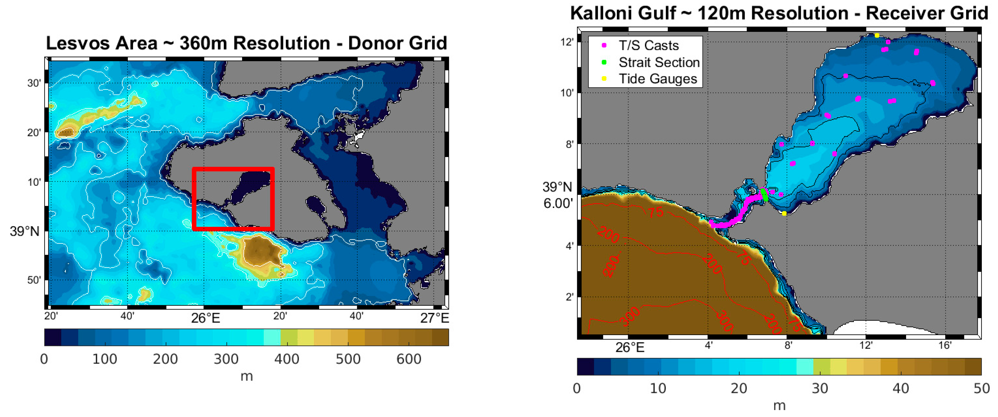
2.3. Numerical Simulations

The circulation model selected for the numerical simulation was the Regional Ocean Modeling System (ROMS 3.7) [22,23,24]). We developed a two-way nested simulation, fully exploiting the model’s capabilities with a refinement ratio of 1:3. The donor (or parent) grid had a horizontal resolution of approximately 360 meters and 30 vertical sigma levels. The receiver (or child) grid had a horizontal resolution of 120 meters with the same number of vertical levels (Figure 3). The donor’s grid-bathymetry was taken from the General Bathymetric Chart of the Oceans (GEBCO) 2014 database and that of the receiver from a digitized high-resolution naval map issued by the Hellenic Navy Hydrographic Service. A minimal selective smoothing was conducted for both grids’ bathymetry, setting the rx0 number [25] to be less than 0.4, particularly 0.35. The logarithmic law of wall was applied for the bottom stresses using a coefficient of 5×10⁻⁴. The selection came after several sensitivity test runs, and this value gave the smallest RMSE for sea surface height when compared with the tide gauges.

For momentum advection, the default third-order upstream bias scheme [26] was used with a weak Laplacian operator for stability. For tracers’ advection the sign preserving MPDATA scheme [27] also with a Laplacian operator along constant geopotential surfaces was used. The vertical mixing scheme of our choice was the classical Mellor – Yamada MY 2.5 [28] using the default background values for eddy viscosity and diffusivity. Boundary and initial conditions (temperature, salinity, sea surface height, u and v velocities) came from a regional scale ocean model of the Aegean Sea [29] locally developed and maintained (unpublished work), using mixed radiation—nudging conditions [30] for 3D fields (T, S, u, v), Chapman [31] for free surface (ζ), and Flather [32] for barotropic velocities (ubar, vbar). The riverine inputs for Kalloni Gulf are climatological daily time-series from a hydrological model covering the period 2003–2016 [33]. Atmospheric forcing comes from the European Centre for Medium-Range Weather Forecasts (ECMWF) ERA5 reanalysis dataset [34] and is incorporated in the model using COARE bulk formulas [35]. Finally, the harmonics for 13 tidal constituents (O1, K1, Q1, P1, M2, S2, N2, K2, MS4, M4, MN4, MF, MM) were obtained from Oregon State University Global Inverse Tidal Model [36].

The simulation covers the period from 1 January, 2018 to 31 July, 2019, initializing with a cold start (no spin up) as we consider that because of the small depths, the Kalloni Gulf converges to and enters a quasi-steady state after a few days.

3. Results

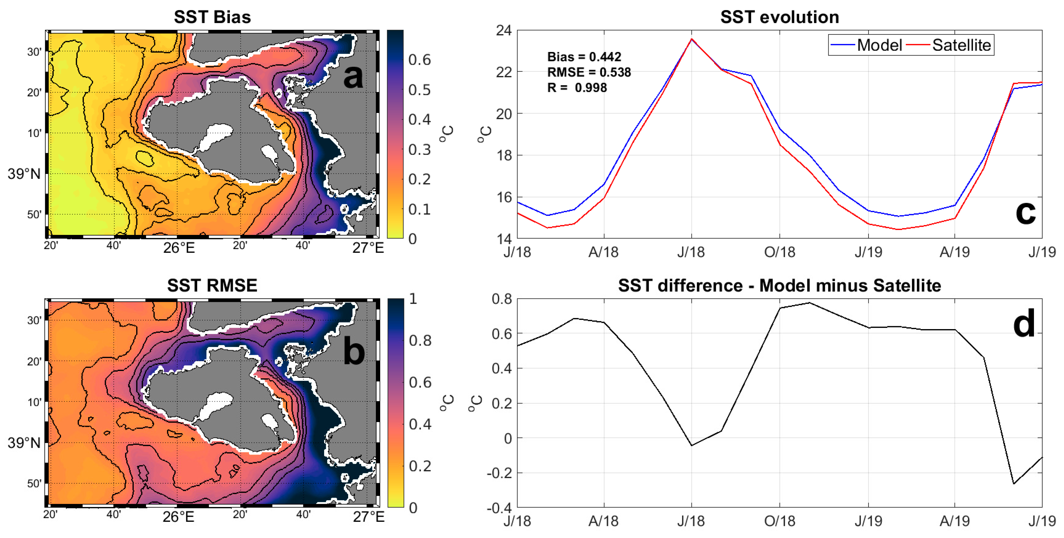
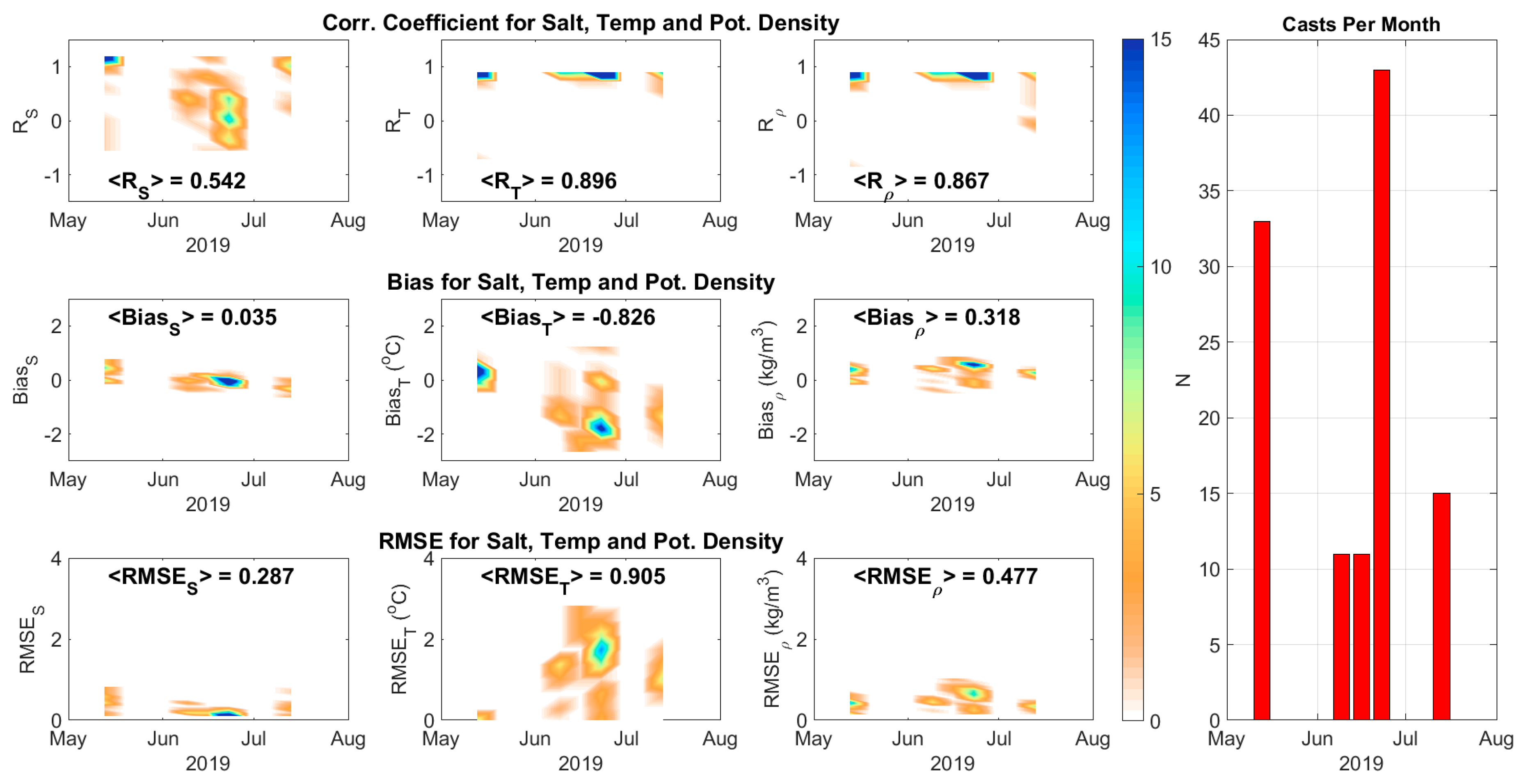
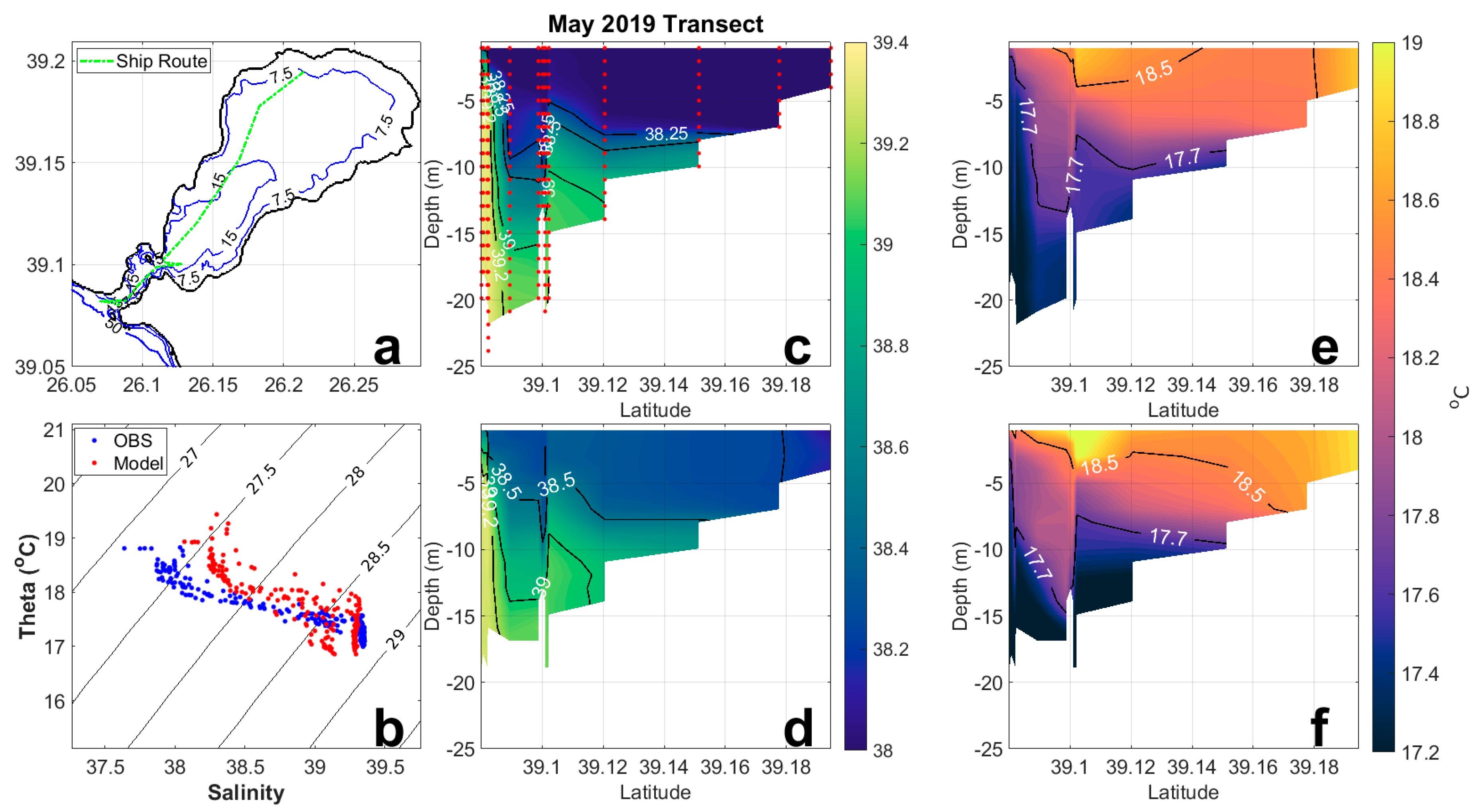
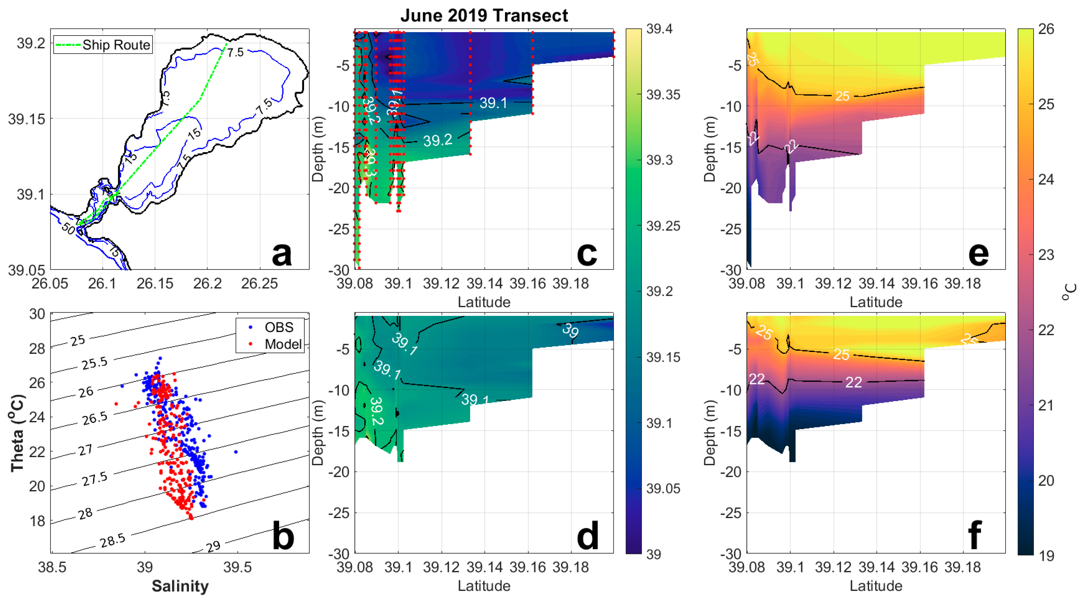
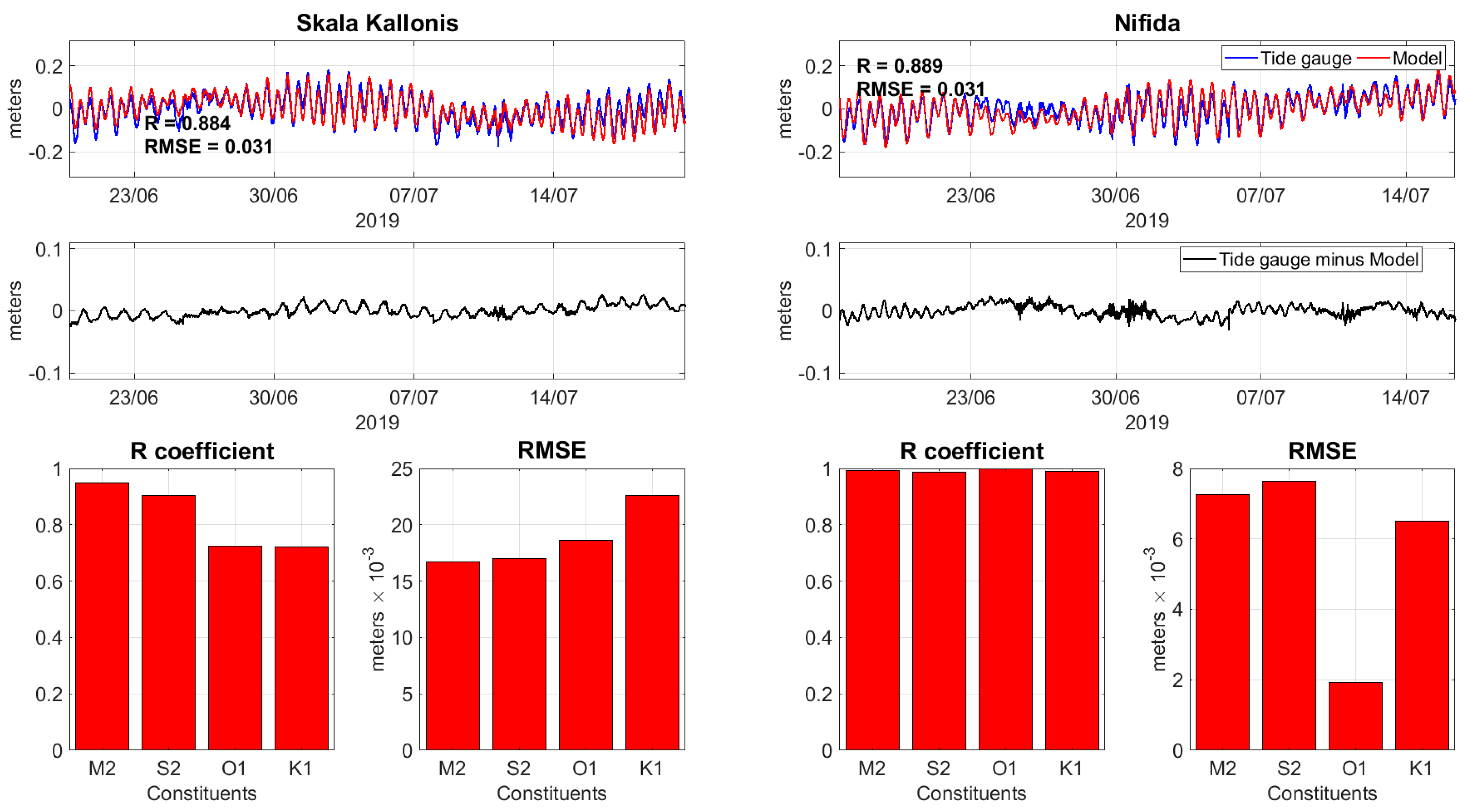
3.1. Model Validation

In order to validate the model’s results, we conducted a typical statistical analysis and comparison with the available in situ field data from surveys and altimetry data (sea surface temperature) for the period of simulation. The statistical metrics used are root mean square error (RMSE), bias skill and Pearson correlation coefficient. Here it must be clarified that the significance of each statistical metric varies according to the physical quantity we analyze and/or compare, i.e., in T/S profile comparison, RMSE and bias skill give a better and more thorough idea for model results than correlation coefficient, R.

The first comparison refers to the sea surface temperature (SST) of the donor grid. We compared the modelled SST with high/ultra-high spatial resolution (0.01 degrees) data from the Copernicus ocean service (product: Mediterranean Sea—High Resolution L4 Sea Surface Temperature Reprocessed, [37,38]). The results from the comparison for each grid point and for the whole basin are presented in Figure 4. The positive mean value of bias for each analysis shows that the donor model overestimates SST and has an RMSE of 0.5 °C magnitude. An interesting fact revealed by Figure 4d is that during winter months there is a systematic overestimation of SST, approximately equal to 0.04 °C and 0.19 °C for July 2018 and June–July 2019, respectively. The highest agreement between modelled and observed SST measures takes place during the periods of maximum stratification of the water column in late spring/summer. These differences have a direct impact on the thermohaline characteristics of Kalloni Gulf, and particularly to temperature distribution.

Figure 5 reveals the impact of the previous mentioned differences in sea surface temperature. The positive SST difference during May gives the smallest scores for RMSE and bias at temperature profiles for the same month. The negative sign difference mainly for June and secondarily for July worsens them because most of the profiles are along the strait that connects Kalloni Gulf to the Aegean Sea, where there is strong horizontal variability.

The salinity and temperature distribution along the major axis of Kalloni Gulf (including the strait) from CTD casts and model for May and June 2019 is presented in Figure 6 and Figure 7, confirming the previous results.

Both figures reveal that the model reproduces quite well the water-mass properties, as well as spatial distribution in the gulf and the strait. The depth of the isotherms and isohalines suggest that most of the mixing takes place at the narrowest point near the southern end of the strait, a feature well-reproduced by the model. Discontinuities in the vertical position of some isothermals and isohalines (most evident in Figure 6) are caused by temporal distancing of some neighboring stations.

Tidal processes seem to play a significant role for the function of Kalloni Gulf. Although the magnitude of tides in the Aegean Sea is small and considered to be insignificant, for a small semi-enclosed embayment like Kalloni, tides may be crucial for the exchanges with the Aegean. We compared the model sea surface height results with two tide gauges installed at the south (Nifida port) and north (Skala Kallonis) parts of the gulf (Figure 1 and Figure 3). Figure 8 and Figure 9 show that the model reproduces adequately the tidal signal and dominant harmonics. The results from the harmonic analysis (conducted using the UTIDE package [39] for MATLAB) are shown in

Table 2. Harmonic analysis results for Nifida.

Harmonic	Method	Percentile Energy (%)	Amplitude (m)	Phase (degrees)
M2	Tide Gauge: ROMS:	57.76 57.30	0.0555 0.0609	61.2 55.0
S2	Tide Gauge: ROMS:	8.41 14.59	0.0212 0.0307	91.3 81.0
K1	Tide Gauge: ROMS:	22.47 22.30	0.0347 0.0380	333.8 332.0
O1	Tide Gauge: ROMS:	4.14 3.06	0.0149 0.0141	304.0 300.0

and

Table 3. Harmonic analysis results for Skala Kallonis.

Harmonic	Method	Percentile Energy (%)	Amplitude (m)	Phase (degrees)
M2	Tide Gauge: ROMS:	54.79 61.34	0.0583 0.0604	64.0 58.1
S2	Tide Gauge: ROMS:	8.39 11.21	0.0228 0.0266	93.2 82.3
K1	Tide Gauge: ROMS:	20.17 16.71	0.0354 0.0301	335.8 334.3
O1	Tide Gauge: ROMS:	3.67 1.53	0.0151 0.0101	304.8 301.0

.

Note that the difference between observed and modelled sea level is very small, of the order of 0.01 m, and is dominated by a daily signal at Skala Kallonis, and by a semi-diurnal signal at Nifida. This difference is attributed to non-tidal, wind-forced sea-level variability related to the daily cycle of sea breeze, a local-scale phenomenon inadequately reproduced by the atmospheric forcing grid of 30-km resolution. Note that the semi-diurnal cycle of the difference at Nifida is attributed to the complicated topography, with sea areas both to the north (the interior of the gulf) and to the south (the open sea) of the site, possibly generating a double-peaked response daily. This effect will be investigated in more detail in the future, as it is outside the scope of this work.

3.2. Water Net Exchange through the Strait

The net exchange at the strait, as estimated using the various methods described in Section 2.1 and Section 2.3, are presented in Figure 9.

The net volume flux estimates provided by the bottom-mounted ADCP method and the sea-level-change methods exhibit an impressive agreement (Figure 9). Note that despite the fact that the sea-level gauge is located at the farthest point of the gulf relative to its entrance, there appears to be no significant phase difference between the results of the two methods, signifying that the sea-level signal is transported very fast to the other end of the Gulf. Thus, both methods can provide acceptable estimates of the net exchange through the strait. Furthermore, the two simulated fluxes (the “long” transect, along the cable, and the “short” transect, across the strait) are indistinguishable (as expected), which suggests that the cable method should provide good estimates for the exchange. However, this is not the case for the estimates produced by the vessel-borne ADCP along-transect method. ADCP values are generally quite noisy, which is why temporal averaging is generally used to provide statistically significant velocity estimates. The short width of the strait led to a choice of short time-averaging for each velocity profile, ranging from 30 seconds in the first transects of May 2019, to the settled value of 10 seconds for the remaining transects (Table 1). Additional errors are introduced by the method of bottom-referencing the velocity fields, either bottom or vessel tracking, in which both can result in noisy parameters. Despite the rather good agreement between the vessel-tracking and bottom-tracking methods regarding the cross-strait velocity fields (Figure 2, top panels), the integrated transport estimates diverge significantly and exhibit great variance when compared to the corresponding estimates provided by the other methods (Figure 9). It should be noted that using longer temporal averages in the post-processing stage did not significantly improve these estimates.

Based on its excellent agreement with the direct method of estimating net exchange via bottom-mounted ADCP, and its capacity to safely and at low-cost provide consistent estimates of net exchange at the strait, the method of sea-level monitoring was selected and is hereafter used as the reference method for assessing net fluxes.

3.3. Telephone Cable Data

The voltage data obtained by the telephone cable method are presented in Figure 10, overlaid on the net exchange estimated based on the sea-level variability method. It is of interest that the cable time-series is dominated by a low-frequency variability, of much larger variance than the tidal signal, in contrast to the net exchange at the strait by the reference method, which is clearly dominated by the tidal signal.

As the electric voltage difference between two coasts is a function not only of the net volume exchange but also of the mean conductivity of the exchanged waters and the seabed, as well as potential leaks in the circuitry and defective grounding of the cables, we decided to investigate if the voltage time-series conceals a useful signal correlated to the tidally-dominated water exchange, since none of the above-described factors would be characterized by a tidal frequency. To investigate this, the spectra of the voltage and reference net volume exchange time-series were computed (Figure 11).

While the net volume flux is dominated by both a diurnal and semidiurnal signal, and the semidiurnal tide is clearly more energetic than the diurnal, this is not the case in the cable signal, which contains a diurnal signal, but lacks a strong semidiurnal peak.

Thus, the facts that (a) the semidiurnal tide is not captured by the cable and (b) the dominance of a low-frequency noise unrelated to volume exchanges suggest that a direct calibration of the cable in order to provide net exchange estimates is not possible yet at this stage. However, in order to fully exploit all possibilities before rejecting the attempt to calibrate the cable, a harmonic analysis was performed for both of the above time-series, and then the synthetic tidal signals were reconstructed based on the four major tidal constituents. The results, presented in Figure 12, certify the lack of semidiurnal signal in the cable time-series, and thus the inability to correctly predict tidal exchange through the Strait. However, Figure 12 reveals an impressive agreement of the temporal evolution of the “beating” pattern between the time-series, presenting a minimal tidal exchange on 27 June, and maximal exchange on 20 June and about 4 July. It is beyond the scope of this work to further investigate this, as well as seek to quantify the possible role of the conductivity variability of water and sediment in the dominance of the low-frequency signal in the cable voltage time-series.

4. Discussion

This work was a testbed for several different methods in developing coastal tools for building a prototype Coastal Observatory.

One of our basic aims was to obtain good voltage difference estimates between the opposing coasts of the strait, in conjunction with net volume flux of water through the strait, in order to calibrate the submarine telephone cable method and proceed to incorporate it in the Coastal Observatory, employing it in detailed assessments of the water volume budgets. The results of the voltage measurements were not encouraging, as the tidal signal was overwhelmed by a low-frequency variability, possibly associated with changes in the electric conductivity of the seabed and/or potential failures of the continuity or leaks of the circuitry. Through collaboration with the telephone cable operators and improvement of our local facilities, we aim to improve and possibly minimize the noise of the measurements. However, this is not expected to completely solve the issue of calibration of the telephone cable method. As shown above, and in agreement with previous observations, the gulf frequently alters its functioning from dilution to concentration basin, and its salinity can exhibit a very large range of seasonal variability, from 37 in the winter to greater than 40 in late summer. Thus, the induced voltage difference can exhibit significant variability, not just due to volume flux changes, but also due to the salinity of the transported waters. It is clear that, when all possible hardware-related problems have been solved, incorporation of the underwater telephone cable in the arsenal of the Coastal Observatory will require a time-dependent (or conductivity-dependent) calibration effort. This work was a first step, contributing with the development, comparison and assessment of three independent methods providing reference estimates of the net volume flux through the Strait.

The method of using vessel-borne ADCP in order to record the spatial variability of the along-strait velocity produced very high transport estimates and was rejected. The failure of the method was attributed to highly noisy velocity estimates, arising both from too-short temporal averages of profiles, as well as noisy vessel positioning and estimation of bottom velocity. However, using longer time-averages to obtain more significant velocity profiles would minimize lateral resolution along the transects, thus overall cancelling the reason for performing them.

On the contrary, the two other methods (the direct method, using a moored ADCP, and the indirect method, via recording the sea-level change of the basin) produced impressive agreement and both can be used to provide reference volume net fluxes.

The use of the former method is based on the assumption of horizontal homogeneity across the strait. The assumption is quite valid, based on the following three arguments: (a) the small width of the strait, of the order of hundreds of meters, which is much less than the baroclinic Rossby radius, (b) the impressive agreement with the sea-level-change method, and (c) the high degree of horizontal homogeneity observed through the cross-strait transects performed through the implementation of the first method.

The sea-level-change method is valid only on relatively short time scales, of the order of tens of days, due to the assumption that the sea-level variability balances the exchange flow at the strait, thus neglecting the atmospheric and land water fluxes. This assumption proved to be very good for the time scales and for the time period addressed in the present work, however, for longer time periods and during the rainy season the validity would fail, as evaporation precipitation and riverine input would become increasingly important. Episodes of climatologically high values of precipitation and riverine runoff in Kalloni Gulf contribute to the water budget of the region with about 0.01 cm in 6 hours, while the evaporation ranges to about 0.002 m in 6 hours, signals much smaller than tidal variability. Thus, while in the summer, the simplification leading to Equation (2) can safely be adopted, during strong rainfall events the full water budget should be considered. Overall, this work has shown that this method is applicable for time periods of the order of several days and in the absence of heavy rainfall, and since it requires minimal effort and investment, it has already been incorporated in the Coastal Observatory of Kalloni Bay, through the installation of a permanent sea-level gauge in the Skala Kallonis harbor in September 2019. The continuous recording of high-frequency sea-level variability in the Gulf will provide us with the means to assess and calibrate the submarine telephone cable method, once all the problems introducing low-frequency noise have been solved.

The model developed for simulating coastal circulation in the Gulf of Kalloni adequately reproduced both the hydrographic properties within the gulf, as well as the net volume exchanges and mixing processes through the connecting strait. The circulation model can constitute the basis for short-term operational forecasting of the gulf’s circulation, as well as long-term climatic projections. Furthermore, the model can be used as a supportive tool for developing a comprehensive coastal management policy, assessing the impact of potential human intervention such as the construction of water reservoirs, ports and additional aquaculture installations.

The selection of a reliable reference method to estimate net exchanges over time scales of the order of tens of days, combined with the development of a model adequately simulating both the hydrographic characteristics and the tidal exchanges through the strait, will enable the further investigation (possibly via modelling) of the possible contribution of salt fluxes through the strait in the low-frequency signal dominating the cable signal. The long-term calibration of cable measurements in straits such as the Florida Keys is possible due to the minor variability of the mean conductivity of the water flowing over the cable. In the case of Kalloni Gulf, or other enclosed basins exhibiting a similar alternating behavior between concentration and dilution, the wide range of salinity and temperature may impose a signal reflecting the conductive flux variability through the strait. Further development of the Coastal Observatory (through the installation of permanent sea-level gauges and the employment of an in situ observation platform and numerical forecasting on a regular basis) will enable the in-depth investigation of the behavior of the cable facility and possibly its incorporation in the observatory.

Thus, future work will build on the herein developed basin-circulation model and exchange-assessment knowledge to expand our understanding of the variability of the net exchange, as well as the inflow and outflow through the strait at seasonal times scales, tightly related to the alternate functioning of the gulf as a concentration and dilution basin. This will significantly contribute to our understanding of the hydrodynamics of the gulf and forming a knowledge base for ecological and biogeochemical studies of the region. Another, parallel effort will be dedicated to expanding our current observations and modeling in developing a concise methodological study and description of recurring hydrodynamics processes in the gulf, such as tidal/current interactions [40]. The latter approach could also be incorporated in our arsenal of methodological tools for studying enclosed and semi-enclosed coastal basins.

Furthermore, the present work has shown that for any enclosed and semi-enclosed basins of similar size (significantly smaller than the barotropic Rossby number), a single site for monitoring the sea-level is the most reliable and cost-effective way to assess net exchanges with the open sea during the dry season and for time-scales of the order of 10 days or less, and thus provide a reference method for the use of submarine telephone cables to assess the exchange at the connecting straits. However, at longer time-scales, water exchanges with the atmosphere and the surrounding catchment area need to be considered, while salinity and temperature variability pose the need to develop seasonally-varying calibration curves.

5. Conclusions

This work describes the first stages in developing a Coastal Observatory, based on the combination of field observations and numerical simulations focused on Kalloni Gulf of Lesvos Island, Greece.

Preliminary results to use a submarine telephone cable laid on the sea-bed across the strait connecting the gulf with the open sea failed, probably due to leaking connections and/or high contribution of a variably conducting seabed on the signal.

Three different methods to assess the net volume exchange at the strait were developed, compared and assessed. The method of performing ADCP transects across the strait failed to provide stable transport estimates due to highly noisy velocity profiles. The method of using an upward-looking, bottom-mounted ADCP produced transport estimates exhibiting very good agreement with the method based on sea-level changes. The latter was selected as the most suitable method for the provision of estimates of the net exchange through the connecting strait, assuming it is applied in time scales of the order of tens of days.

The numerical model developed for pre-operational simulations of the gulf’s circulation and exchanges with the open sea reproduces adequately the hydrographic conditions in the gulf, as well as the volume exchanges at the strait. The model is considered ready for operational use; furthermore, its results will be integrated in a future cable calibration attempt, where the temporal variability of seawater conductivity on a seasonal basis will be taken into consideration.

References

1. Healy, T.; Harada, K. Enclosed and Semi-Enclosed Coastal Seas. J. Coastal Res. 1991, 7, i–iv. Available online: www.jstor.org/stable/4297799 (accessed on 25 February 2020).
2. Garvine, R.W.; Whitney, M.M. An estuarine box model of freshwater delivery to the coastal ocean for use in climate models. J. Mar. Res. 2006, 64, 173–194. [Google Scholar] [CrossRef]
3. Hordoir, R.; Polcher, J.; Brun-Cottan, J.-C.; Madec, G. Towards a parametrization of river discharges into ocean general circulation models: A closure through energy conservation. Clim. Dyn. 2008, 31, 891–908. [Google Scholar] [CrossRef]
4. Verri, G.; Pinardi, N.; Bryan, F.; Tseng, Y.; Coppini, G.; Clementi, E. A box model to represent estuarine dynamics in mesoscale resolution ocean models. Ocean Model. 2020, 148, 101587. [Google Scholar] [CrossRef]
5. Raicevich, S.; Barausse, A.; Canadelli, E.; Fortibuoni, T.; Mazzoldi, C. Historical Ecology of Semi-Enclosed Basins and Coastal Areas: Past, Present and Future of Seas at Risk; Regional Studies in Marine Science; Elsevier: Amsterdam, the Netherlands, 2018; Volume 21, pp. 1–102. [Google Scholar] [CrossRef]
6. Caddy, J. Marine catchment basin effects versus impacts of fisheries on semi-enclosed seas. ICES J. Mar. Sci. 2000, 57, 628–640. [Google Scholar] [CrossRef] [Green Version]
7. Petihakis, G.; Triantafyllou, G.; Korres, G.; Tsiaras, K.; Theodorou, A. Ecosystem modelling: Towards the development of a management tool for a marine coastal system part-II, ecosystem processes and biogeochemical fluxes. J. Mar. Syst. 2012, 94, S49–S64. [Google Scholar] [CrossRef]
8. Tintoré, J.; Pinardi, N.; Álvarez-Fanjul, E.; Aguiar, E.; Álvarez-Berastegui, D.; Bajo, M.; Balbin, R.; Bozzano, R.; Nardelli, B.B.; Cardin, V.; et al. Challenges for sustained observing and forecasting systems in the mediterranean sea. Front. Mar. Sci. 2019, 6, 568. [Google Scholar] [CrossRef] [Green Version]
9. Martín Míguez, B.; Novellino, A.; Vinci, M.; Claus, S.; Calewaert, J.-B.; Vallius, H.; Schmitt, T.; Pititto, A.; Giorgetti, A.; Askew, N.; et al. The European marine observation and data network (EMODnet): Visions and roles of the gateway to marine data in Europe. Front. Mar. Sci. 2019, 6, 313. [Google Scholar] [CrossRef] [Green Version]
10. Puillat, I.; Farcy, P.; Durand, D.; Karlson, B.; Petihakis, G.; Seppälä, J.; Sparnocchia, S. Progress in marine science supported by European joint coastal observation systems: The JERICO-RI research infrastructure. J. Mar. Syst. 2016, 162, 1–3. [Google Scholar] [CrossRef] [Green Version]
11. Panayotidis, P.; Feretopoulou, J.; Montesanto, B. Benthic Vegetation as an Ecological Quality Descriptor in an Eastern Mediterranean Coastal Area (Kalloni Bay, Aegean Sea, Greece). Estuar. Coast. Shelf Sci. 1999, 48, 205–214. [Google Scholar] [CrossRef]
12. Spatharis, S. Phytoplankton Diversity and Bloom Dynamics in Coastal Ecosystems under the Influence of Terrestrial Runoff. Ph.D. Thesis, University of the Aegean, Mytilene, Greece, 2007. [Google Scholar]
13. Debenay, J.-P. Relationships between foraminiferal assemblages and hydrodynamics in the Gulf of Kalloni, Greece. J. Foraminifer. Res. 2005, 35, 327–343. [Google Scholar] [CrossRef]
14. Leroi, A.M. The Lagoon: How Aristotle Invented Science; Penguin Books: London, UK, 2015; ISBN 9780143127987. [Google Scholar]
15. Zenetos, A.; Papathanassiou, E. Community parameters and multivariate analysis as a means of assessing the effects of tannery effluents on macrobenthos. Mar. Pollut. Bull. 1989, 20, 176–181. [Google Scholar] [CrossRef]
16. Diapoulis, A.; Bogdanos, K.; Haritonidis, S.; Konidis, A. The impact of pollution on the synthesis of the coastal benthos in the culf of Kalloni (Lesvos Island, Greece). Fresenius Environ. Bull. 1998, 7, 146–152. [Google Scholar]
17. Kefalas, E.; Castritsi-Catharios, J.; Miliou, H. The impacts of scallop dredging on sponge assemblages in the Gulf of Kalloni (Aegean Sea, northeastern Mediterranean). ICES J. Mar. Sci. 2003, 60, 402–410. [Google Scholar] [CrossRef]
18. Spatharis, S.; Danielidis, D.B.; Tsirtsis, G. Recurrent Pseudo-nitzschia calliantha (Bacillariophyceae) and Alexandrium insuetum (Dinophyceae) winter blooms induced by agricultural runoff. Harmful Algae 2007, 6, 811–822. [Google Scholar] [CrossRef]
19. Zanou, B.; Kopke, A. Cost-effective reduction of eutrophication in the Gulf of Kalloni (Island of Lesvos, Greece). Med. Mar. Sc. 2001, 2, 15. [Google Scholar] [CrossRef] [Green Version]
20. Hughes, P. Submarine Cable Measurements of Tidal Currents in the Irish Sea. Limnol. Oceanogr. 1969, 14, 269–278. [Google Scholar] [CrossRef]
21. Sanford, T.B. Motionally induced electric and magnetic fields in the sea. J. Geophys. Res. 1971, 76, 3476–3492. [Google Scholar] [CrossRef]
22. Haidvogel, D.B.; Arango, H.G.; Hedstrom, K.; Beckmann, A.; Malanotte-Rizzoli, P.; Shchepetkin, A.F. Model evaluation experiments in the North Atlantic Basin: Simulations in nonlinear terrain-following coordinates. Dyn. Atmos. Oceans 2000, 32, 239–281. [Google Scholar] [CrossRef]
23. Shchepetkin, A.F.; McWilliams, J.C. A method for computing horizontal pressure-gradient force in an oceanic model with a nonaligned vertical coordinate. J. Geophys. Res. 2003, 108, 3090. [Google Scholar] [CrossRef]
24. Shchepetkin, A.F.; McWilliams, J.C. The Regional Ocean Modeling System: A split-explicit, free-surface, topography following coordinates ocean model. Ocean Model. 2005, 9, 347–404. [Google Scholar] [CrossRef]
25. Haidvogel, D.B.; Beckmann, A. Numerical Ocean Circulation Modeling; Series on Environmental Science and Management; Imperial College Press: London, UK, 1999; Volume 2. [Google Scholar] [CrossRef]
26. Shchepetkin, A.F.; McWilliams, J.C. Quasi-monotone advection schemes based on explicit locally adaptive dissipation. Mon. Weather Rev. 1998, 126, 1541–1580. [Google Scholar] [CrossRef]
27. Smolarkiewicz, P.K.; Margolin, L.G. MPDATA: A Finite-Difference Solver for Geophysical Flows. J. Comput. Phys. 1998, 140, 459–480. [Google Scholar] [CrossRef] [Green Version]
28. Mellor, G.L.; Yamada, T. Development of a turbulence closure model for geophysical fluid problems. Rev. Geophys. Space Phys. 1982, 20, 851–875. [Google Scholar] [CrossRef] [Green Version]
29. Mamoutos, I.G.; Zervakis, V.; Tragou, E. The role of residual currents on the Aegean Sea. manuscript under preparation.
30. Marchesiello, P.; McWilliams, J.C.; Shchepetkin, A.F. Open boundary conditions for long-term integration of regional ocean models. Ocean Model. 2001, 3, 1–20. [Google Scholar] [CrossRef]
31. Chapman, D.C. Numerical treatment of cross-shelf open boundaries in a barotropic coastal ocean model. J. Phys. Oceanogr. 1985, 15, 1060–1075. [Google Scholar] [CrossRef] [Green Version]
32. Flather, R.A. A tidal model of the northwest European continental shelf. Mem. de la Soc. R. de Sci. de Liege 1976, 6, 141–164. [Google Scholar]
33. Chalazas, T.; Tzoraki, O.; Cooper, D.; Efstratiou, M.A.; Bakopoulos, V. Ecosystem service evaluation of streams for nutrients and bacteria purification in a grazed watershed. Fresenius Environ. Bull. 2017, 26, 7849–7859. [Google Scholar]
34. Copernicus Climate Change Service (C3S) (2017): ERA5: Fifth generation of ECMWF atmospheric reanalyses of the global climate. Copernicus Climate Change Service Climate Data Store (CDS), 2019. Available online: https://cds.climate.copernicus.eu/cdsapp#!/home (accessed on 10 September 2019).
35. Fairall, C.W.; Bradley, E.F.; Rogers, D.P.; Edson, J.B.; Young, G.S. Bulk parameterization of air-sea fluxes for tropical ocean-global atmosphere Coupled-Ocean Atmosphere Response Experiment. J. Geophys. Res. 1996, 101, 3747–3764. [Google Scholar] [CrossRef]
36. Egbert, G.D.; Erofeeva, Y.S. Efficient inverse modeling of barotropic ocean tides. J. Atmos. Ocean. Technol. 2002, 19, 183–204. [Google Scholar] [CrossRef] [Green Version]
37. Pisano, A.; Buongiorno Nardelli, B.; Tronconi, C.; Santoleri, R. The new Mediterranean optimally interpolated pathfinder AVHRR SST Dataset (1982–2012). Remote Sens. Environ. 2016, 176, 106–117. [Google Scholar] [CrossRef]
38. Buongiorno Nardelli, B.; Tronconi, C.; Pisano, A.; Santoleri, R. High and Ultra-High resolution processing of satellite Sea Surface Temperature data over Southern European Seas in the framework of MyOcean project. Remote Sens. Environ. 2013, 129, 1–16. [Google Scholar] [CrossRef]
39. Codiga, D. UTide Unified Tidal Analysis and Prediction Functions. 2020. Available online: https://www.mathworks.com/matlabcentral/fileexchange/46523-utide-unified-tidal-analysis-and-prediction-functions (accessed on 16 January 2020).
40. Armenio, E.; De Serio, F.; Mossa, M. Analysis of data characterizing tide and current fluxes in coastal basins. Hydrol. Earth Syst. Sci. 2017, 21, 3441. [Google Scholar] [CrossRef] [Green Version]
Figure 1. (a) Map of the Aegean Sea, connecting the Mediterranean and the Black Sea. The rectangle identifies Lesvos Island, whose center is dominated by Kalloni Gulf. (b) Bathymetric map of Kalloni Gulf, with contours every 5 m. The locations of the Acoustic Doppler Current Profiler (ADCP) station (red dot), the bottom-pressure gauges (cyan dots) and the voltage-meter station (blue square) are identified. In the inset box, a close-up of the Kalloni Strait is shown. The cable line (“long”) and the across-strait (“short”) transects are identified by the purple and yellow lines respectively.
Jmse 08 00336 g001
Figure 2. Top: Cross-transect velocity as recorded by the shipborne ADCP, referring to the bottom via vessel-tracking (left), bottom-tracking (middle) and numerical model (right) methods. Positive values signify inflow to the gulf. Bottom: Vertically integrated, seabed-referred velocities using vessel-tracking (left), bottom-tracking (middle) and numerical model (right).
Jmse 08 00336 g002
Figure 3. Left: Bathymetry of donor’s grid covering Lesvos area. Right: Kalloni Gulf (receiver grid) bathymetry and limits. Magenta dots show CTD casts through May, June and July 2019 surveys, green dots indicate the strait section from where several quantities were calculated from model outputs and compared with collected data, and yellow dots are the positions of two tide gauges stations at Nifida (south) and Skala Kallonis (north).
Jmse 08 00336 g003
Figure 4. (a) Sea surface temperature (SST) bias for each grid point. (b) Root mean square error (RMSE) for every grid point. (c) Basin’s monthly mean SST values, model and satellite. (d) Mean SST difference (model − satellite observation).
Jmse 08 00336 g004
Figure 5. Comparison between observed and modelled T/S profiles for Kalloni Gulf for May, June and July 2019. Positions of casts are given in Figure 2 (right panel).
Jmse 08 00336 g005
Figure 6. May 2019 along strait transect. Upper left (a), ship route along strait; lower left (b), T/S diagram for observed and modelled profiles. Upper middle (c) and right (e), observed salinity and temperature. Lower middle (d) and right (f), modelled salinity and temperature.
Jmse 08 00336 g006
Figure 7. June 2019 along strait transect. Upper left (a), ship route along strait; lower left (b), T/S diagram for observed and modelled profiles. Upper middle (c) and right (e), observed salinity and temperature. Lower middle (d) and right (f), modelled salinity and temperature.
Jmse 08 00336 g007
Figure 8. Sea surface height comparison (top row), difference between observed and modelled sea level (middle row), and correlation coefficient and RMSE for the dominant harmonics (bottom row) at Skala Kallonis (left) and Nifida (right).
Jmse 08 00336 g008
Figure 9. Net volume exchange at the strait, as estimated by the moored ADCP method (black line), the sea-level change method (green line), the shipborne ADCP method (dots), and as simulated across the long (red line) and the short (blue line) transects. For the latter method, both the vessel-tracking (red/purple) and bottom-tracking (blue/light blue) results are presented, as well as estimates of both long transects (+) and short transects (o). The whole period from May to July is presented in the top panel, while the lower panel provides a focus on the June 2020 cruises where we have simultaneous use of all three methods. The positive sign of the transport denotes inflow to the gulf.
Jmse 08 00336 g009
Figure 10. Time-series of telephone cable voltage (blue and net exchange based on the reference sea-level change method (green). The latter’s low-passed time-series is shown in red.
Jmse 08 00336 g010
Figure 11. Spectra of the net-exchange volume flux based on the reference method (left) and the cable voltage (right).
Jmse 08 00336 g011
Figure 12. Synthetically constructed time-series of net volume exchange through the strait (green) and cable voltage (blue), using the four main tidal constituents after harmonic analysis of the signals.
Jmse 08 00336 g012