Seepage Force on a Buried Submarine Pipeline Induced by a Solitary Wave

Abstract

In this study, a finite element method was used to establish a two-dimensional numerical model to solve the problem of the Biot equation describing the poroelastic seabed, and to analyze the seepage force on a buried submarine pipeline under the propagation of a solitary wave. The model provides a solution to the displacement of the poroelastic seabed and the variation of the pore-water pressure. By means of numerical simulation, the effects of Young’s modulus and permeability coefficient of the soil on the pore-water pressure and seepage force are discussed. In the simulation of solitary waves passing through fully buried submarine pipelines, numerical results indicate that the smaller the permeability coefficient in dense sandy bed the greater the vertical force acting on the pipeline, and the smaller the permeability coefficient in loose sand bed the smaller the vertical force acting on the pipeline. In general, when the permeability coefficient is large, the smaller the Young’s modulus the more obvious the influence of the vertical force on the pipeline, and when the permeability coefficient is small, the larger the Young’s modulus the more obvious the influence of the vertical force on the pipeline.

1. Introduction

Buried submarine pipelines are increasingly affecting daily life. Any damage to these pipelines by natural disasters or human factors has a major impact on the economy and society. For example, in 26 December 2006, the Hengchun earthquakes occurred in the Luzon Strait, where multiple international submarine pipelines meet. The turbidity currents triggered by the earthquake damaged the pipelines, resulting in disconnection from the internet and blockage of communication services in East Asia. It also blocked international finance services, causing incalculable financial losses. This example shows that the stability of buried submarine pipelines is a critical topic in marine engineering.

Biot [1] proposed the three-dimensional consolidation theory for poroelastic soil. The basic assumption of this theory is that soil particles comprise homogeneous and isotropic porous media, and water is present in the pores. Furthermore, the solid medium and pore water are compressible. The stress–strain relationship of the solid medium is linear, and the movement of the water in the pores satisfies Darcy’s law.

Massel [2] proposed the use of a nonlinear damper and inertia in the momentum equation to replace Darcy’s law for analysis of stiff porous seabed. Madsen [3] theoretically analyzed the permeability and pore water pressure of an infinitely deep porous seabed and calculated the periodic-wave-induced effective stress in this seabed. Yamamoto et al. [4] used Fourier series expansion and derived analytical solutions of the displacement, pore water pressure, and effective stress of a poroelastic seabed. They discussed saturated and unsaturated sand with infinite depth, and empirical data were employed for verification. Magda [5] proposed an analytical solution of the pore water pressure of a wave passing along seabed with finite depth and used the compressibility of soil and pore fluid to conduct a practicality test. Magda [6] employed a two-dimensional finite-element model to simulate the hydrodynamic force on a buried submarine pipeline as periodic waves passed through the seabed. Magda [7] discussed whether the soil on the seabed and the fluid are compressible to further determine the wave-effect-derived uplifting force and pore pressure on buried submarine pipelines. Wang et al. [8] used element-free Galerkin methods to numerically analyze two-dimensional seabed with finite depth. In addition to evaluating the instant liquidation under different soil and wave conditions, they discussed variation in the stability of the seabed, including wave length, compressibility of the pore fluid, and permeability and stiffness of the porous medium. Liu et al. [9] analyzed the problem of a long wave passing over unsaturated permeable seabed and solved the Navier–Stokes equation for the fluid flow and Darcy’s equation for the pore water flow in the soil.

Regarding the relevant experimental research, Nakamura et al. [10] conducted pore pressure measurement on seabed with fine and coarse sands, and compared the findings with theoretical results. Yamamoto et al. [4] conducted a pore water pressure test using a flume containing soil mixed with fine sand, coarse sand, and a small quantity of air. McDougal et al. [11] noticed discrepancies between the theoretical and experimental values of the pore pressure caused by waves and proposed the following three reasons for these discrepancies: (1) under the premise that pore fluid and soil are incompressible, the potential-flow theory used in numerical calculation could not include all critical and determining parameters of the soil and pore fluid; (2) compared with the soil model experiment conducted in the laboratory, for which the soil has finite thickness, the numerical calculation employed unreasonable boundary conditions, such as a seabed with semi-infinite depth; and (3) the simulation parameters in the numerical calculation and the parameters used in the laboratory model may not have been consistent.

In the past several decades, studies on the wave–seabed interaction have primarily focused on periodic waves. Sumer [12] stated that after the tsunamis caused by the earthquake in the Indian Ocean on 26 December 2004, and by the earthquake in northeastern Japan on 11 March 2011, engineers realized that their knowledge on the interaction between tsunamis, seabed, and underwater constructions was still limited and future research was required. Moreover, studies on the potential pipeline damage and seabed scouring that occur when a tsunami passes a nearshore buried submarine pipeline are few in the literature.

This study employed Biot’s compression theory and the finite-element method to construct a two-dimensional numerical model for determining the influence of a solitary wave on the pore-water pressure in a flat poroelastic seabed. The water in the seabed pores was assumed to be saturated and incompressible. The Young’s modulus and permeability coefficient of the seabed were the major soil parameters considered during analysis. Subsequently, the model was used to analyze the seepage force on a buried submarine pipeline due to excess pore-water pressure. In addition, the change over time of the seepage force under different soil permeability coefficients and Young’s moduli was determined, and this study deduced the relationship between the maximum force on the pipeline and these two parameters.

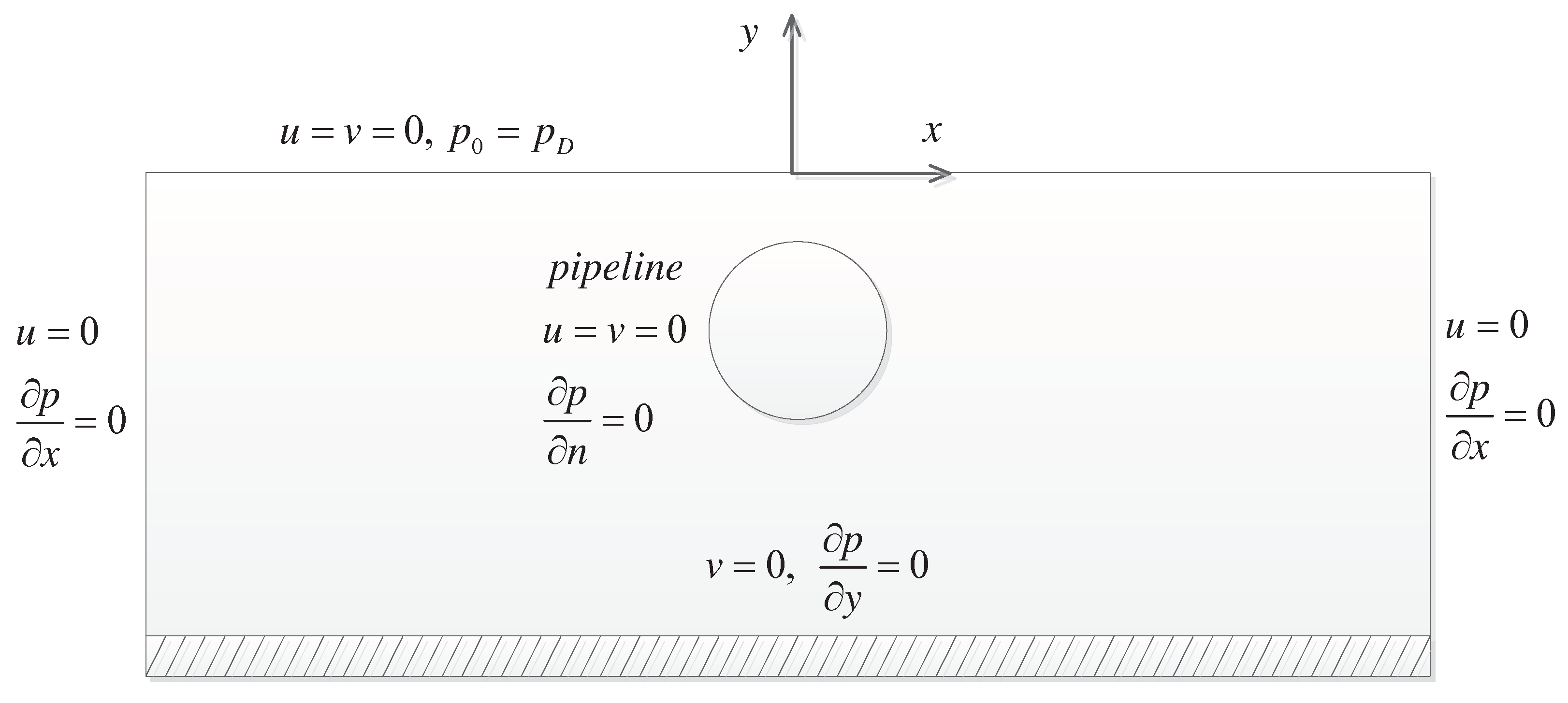
2. Mathematical Formulations

A schematic diagram of the research area of this study is displayed Figure 1, where a is the amplitude of the solitary wave, h is the still water depth, H is the depth of the poroelastic seabed, b is the burial depth of the pipeline, and D is the diameter of the pipeline. The calculation area of this model is the poroelastic seabed. The water pressure produced by the solitary wave is considered to be known and is provided. The soil on the seabed is considered a poroelastic medium that is homogeneous, isotropic, and compressible. The consolidation theory proposed by Biot [1] and storage equation proposed by Verruijt [13] are used to calculate the stress and pore water pressure caused by the solitary wave in the poroelastic soil as well as the seepage force on the pipeline buried under the seabed. The stress–strain relationship satisfies Hooke’s law, and the pore water is assumed to be incompressible and to satisfy Darcy’s law. The governing equations of the two-dimensional problem consist of two linear elastic equilibrium equations and the so-called storage equation:

$$G\left(\frac{{\partial }^{2}u}{\partial x^2}+\frac{{\partial }^{2}u}{\partial y^2}\right)+\frac{G}{1-2\mu }\frac{\partial }{\partial x}\left(\frac{\partial u}{\partial x}+\frac{\partial v}{\partial y}\right)=\frac{\partial p}{\partial x},$$

(1)

$$G\left(\frac{{\partial }^{2}v}{\partial x^2}+\frac{{\partial }^{2}v}{\partial y^2}\right)+\frac{G}{1-2\mu }\frac{\partial }{\partial y}\left(\frac{\partial u}{\partial x}+\frac{\partial v}{\partial y}\right)=\frac{\partial p}{\partial y},$$

(2)

$$\frac{k}{\gamma }\left(\frac{{\partial }^{2}p}{\partial x^2}+\frac{{\partial }^{2}p}{\partial y^2}\right)=\frac{\partial }{\partial t}\left(\frac{\partial u}{\partial x}+\frac{\partial v}{\partial y}\right).$$

(3)

where u and v are the soil displacements in the x- and y-directions, respectively, p is the excess (wave-induced) pore-water pressure, $G=E/\left[2\right(1+\mu \left)\right]$ is the shear modulus for isotropic soil, E is Young’s modulus of elasticity for isotropic soil, $\mu$ is Poisson’s ratio of the soil, k is the coefficient of soil permeability, $\gamma$ is the unit weight of pore fluid, and t is the time.

The boundary conditions are illustrated in Figure 2. Assume that the bottom of the permeable seabed is stiff and impermeable:

$$v=0,$$

(4)

$$\frac{\partial p}{\partial y}=0.$$

(5)

For the convenience of computation, the left and right boundaries are also set to be stiff in the vertical direction and impermeable, like the bottom:

$$u=0,$$

(6)

$$\frac{\partial p}{\partial x}=0.$$

(7)

The lateral boundaries should be far enough away from the pipeline so that the artificial boundary conditions would not affect the results. At the seabed surface, the effect of the relative movement between the water and seabed is neglected, and only the transmission of the water pressure is considered:

$$u=v=0,$$

(8)

$$p=p_D,$$

(9)

where $p_D$ is the dynamic pressure caused by the solitary wave. Under the assumption of hydrostatic pressure distribution,

$$p_D=\gamma \eta ,$$

(10)

where $\eta$ is the free-surface elevation of solitary wave. In this research, Boussinesq’s solution for solitary waves [14] is applied to obtain $\eta$ as

$$\eta =a{\mathrm{sech}}^2\sqrt{\frac{3}{4}\frac{a}{h^3}}(x-ct),$$

(11)

where a is the wave amplitude and $c=\sqrt{g(h+a)}$ is the wave speed. The pipeline is assumed to be fixed in the soil and will not cause disturbance to the seabed. The boundary conditions of the pipeline surface are as follows:

$$u=v=0,$$

(12)

$$\frac{\partial p}{\partial n}=0,$$

(13)

where n is the coordinate normal to the pipeline surface.

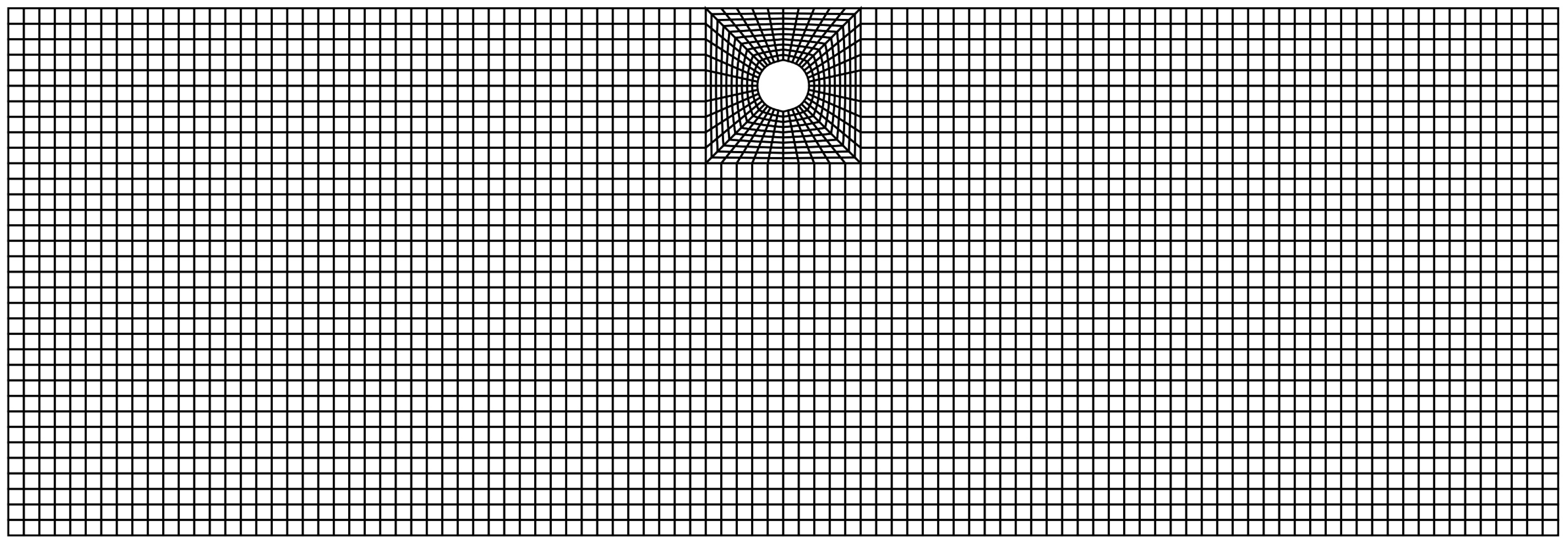
3. Finite-Element Methods

This study employs the finite-element model proposed by Smith et al. [15] to solve Equations (1)–(3) and the corresponding boundary conditions Equations (4)–(13). The displacement of the elastic seabed $(u,v)$ and excess pore water pressure p are determined. When the nodal values of these three variables are discrete, the variables in the elements can be expressed as

$$\tilde{u}=\left[{\mathbf{N}}_u\right]\left\{\mathbf{u}\right\},$$

(14)

$$\tilde{v}=\left[{\mathbf{N}}_u\right]\left\{\mathbf{v}\right\},$$

(15)

$$\tilde{p}=\left[{\mathbf{N}}_p\right]\left\{\mathbf{p}\right\},$$

(16)

where $\left[{\mathbf{N}}_u\right]$ and $\left[{\mathbf{N}}_p\right]$ are the shape functions for the displacement and pore water pressure, respectively, whereas $\left\{\mathbf{u}\right\}$, $\left\{\mathbf{v}\right\}$, and $\left\{\mathbf{p}\right\}$ are the nodal values of each element. The element used is rectangular (Figure 3). Each element has eight displacement nodes (Nodes 1–8) and four water pressure nodes (Nodes 1, 3, 5, and 7). The displacement and pore water pressure shape functions are

$${\left[{\mathbf{N}}_u\right]}^T=\left\{\begin{array}{c}\frac{1}{4}(1-\xi )(1-\eta )(-\xi -\eta -1)\\ \frac{1}{2}(1-\xi )(1-{\eta }^2)\\ \frac{1}{4}(1-\xi )(1+\eta )(-\xi +\eta -1)\\ \frac{1}{2}(1-{\xi }^2)(1+\eta )\\ \frac{1}{4}(1+\xi )(1+\eta )(\xi +\eta -1)\\ \frac{1}{2}(1+\xi )(1-{\eta }^2)\\ \frac{1}{4}(1+\xi )(1-\eta )(\xi -\eta -1)\\ \frac{1}{2}(1-{\xi }^2)(1-\eta )\end{array}\right\},$$

(17)

$${\left[{\mathbf{N}}_p\right]}^T=\left\{\begin{array}{c}\frac{1}{4}(1-\xi )(1-\eta )\\ \frac{1}{4}(1-\xi )(1+\eta )\\ \frac{1}{4}(1+\xi )(1+\eta )\\ \frac{1}{4}(1+\xi )(1-\eta )\end{array}\right\},$$

(18)

where $(\xi ,\eta )$ is the transformed coordinate system.

The Galerkin approximation is used, and then from Equations (1)–(3), a group of equations and a discrete equation of continuous equations are as follows [15]:

$$\left[{\mathbf{k}}_m\right]\left\{\mathbf{u}\right\}-\left[\mathbf{c}\right]\left\{\mathbf{p}\right\}=\left\{\mathbf{f}\right\},$$

(19)

$${\left[\mathbf{c}\right]}^T\left\{\frac{d\mathbf{u}}{dt}\right\}-\left[{\mathbf{k}}_c\right]\left\{\mathbf{p}\right\}=\left\{\mathbf{0}\right\},$$

(20)

where $\left[{\mathbf{k}}_m\right]$ and $\left[{\mathbf{k}}_c\right]$ are the elastic stiffness matrix and fluid conductivity matrix, respectively; $\left[\mathbf{c}\right]$ is the integral of the shape function; $\left\{\mathbf{f}\right\}$ is the external loading vector; $\left\{\mathbf{u}\right\}$ and $\left\{\mathbf{p}\right\}$ are the displacement and pore water pressure of the node element, respectively

$$\left\{\mathbf{u}\right\}={[u_1,v_1,u_2,v_2,u_3,v_3,\dots ,u_8,v_8]}^T,$$

(21)

$$\left\{\mathbf{p}\right\}={[p_1,p_3,p_5,p_7]}^T.$$

(22)

In Equation (19), $\left\{\mathbf{f}\right\}$ is the external force added to the system. In the time interval $[t_0,t_1]$, the variation in external force is $\{\Delta \mathbf{f}\}$, and then the increment of Equation (19) can be expressed as

$$\left[{\mathbf{k}}_m\right]\{\Delta \mathbf{u}\}-\left[\mathbf{c}\right]\{\Delta \mathbf{p}\}=\{\Delta \mathbf{f}\},$$

(23)

where $\{\Delta \mathbf{u}\}$ and $\{\Delta \mathbf{p}\}$ are the variation of the displacement and pore pressure, respectively. Linear interpolation is used in this time interval for $\{\Delta \mathbf{u}\}$, and then

$$\{\Delta \mathbf{u}\}=\Delta t\left((1-\varphi ){\left\{\frac{d\mathbf{u}}{dt}\right\}}_0+\varphi {\left\{\frac{d\mathbf{u}}{dt}\right\}}_1\right),$$

(24)

where $\varphi$ is the weight, generally set to 0.5. This equation is combined with Equation (20) to obtain the following incremental recursive equations:

$$\left[\begin{array}{cc}\left[{\mathbf{k}}_m\right]& -\left[\mathbf{c}\right]\\ {\left[\mathbf{c}\right]}^T& \varphi \Delta t\left[{\mathbf{k}}_c\right]\end{array}\right]\left\{\begin{array}{c}\left\{\Delta \mathbf{u}\right\}\\ \left\{\Delta \mathbf{p}\right\}\end{array}\right\}=\left\{\begin{array}{c}\left\{\Delta \mathbf{f}\right\}\\ \Delta t\left[{\mathbf{k}}_c\right]{\left\{\mathbf{p}\right\}}_0\end{array}\right\}.$$

(25)

After solving the increment from Equation (25), the variables at time $t_1$ can be obtained as

$$\begin{array}{c}\hfill {\left\{\mathbf{u}\right\}}_1={\left\{\mathbf{u}\right\}}_0+\{\Delta \mathbf{u}\}\\ \hfill {\left\{\mathbf{p}\right\}}_1={\left\{\mathbf{p}\right\}}_0+\{\Delta \mathbf{p}\}.\end{array}$$

(26)

Figure 4 illustrates the grid system used to calculate the force on the pipeline under the seabed (see Section 6). Due to the round boundary formed by the pipeline, the boundary-fitted meshes generated using a transfinite interpolation technique [16] is employed within the rectangle zone of the pipeline nearest proximity. Square elements are used outside the rectangle zone. In the cases without the pipeline (Section 5), only square elements are employed.

4. Model Validation

After the model was established, an analytical solution of the one-dimensional soil consolidation problem [17] was compared with the numerical calculation results to verify the accuracy of the proposed model. As Figure 5 shows, the soil model comprised four square meshes that were 1-m deep and 0.25-m wide. A linear load $P_{\mathrm{load}}$ was assumed to act on the surface of the soil and was spatially evenly distributed but varied over time. The grid had eight nodes, each of which had three degrees of freedom. The bottom of the soil and the side boundaries were set to be impermeable boundaries. That is,

$$\frac{\partial p}{\partial n}=0.$$

(27)

The boundary conditions at the sides were fixed, meaning no x-directional displacement. The top of the soil is drained. That is,

$$p=0.$$

(28)

In the solution of Schiffman [17], a nondimensional time factor T is set, which has the following relationship with time t:

$$T=\frac{c_{v}t}{H_{dr}^2},$$

(29)

where $H_{dr}$ is the maximum drainage path, and $c_v$ is the consolidation parameter defined as

$$c_v=\frac{k}{m_v\gamma }$$

(30)

with $m_v$ the coefficient of volume compressibility:

$$m_v=\frac{(1+\mu )(1-2\mu )}{E(1-\mu )}.$$

(31)

For easy comparison with the analytical solutions, during calculation, the effective Young’s modulus was set to $E=1.0$, the effective Poisson’s ratio to $\mu =0$, the ratio of permeability parameter over the unit weight of water to $k/\gamma =1.0$, and the maximum drainage path to $H_{dr}=1$. The coefficient of volume compressibility could then be obtained, $m_v=1.0$, as well as the consolidation parameter, $c_v=1.0$. The time interval for the calculation was set to $\Delta t=0.1$. The loading on the soil surface $P_{\mathrm{load}}$ was set to be linear, increasing at a fixed velocity, and reaching the fixed load $P_{\mathrm{load}}$ at $t_0=0.1$ (Figure 6).

Figure 7 illustrates how the excess pore water pressure changed over time at different depths, as calculated using the model. The pore pressure first increased due to the surface load, and then dissipated because of the drainage at the top of the soil. Figure 7 also illustrates the analytical solution of Schiffman [17] of the excess pore water pressure at the bottom of the soil, which was favorably consistent with the numerical solution. This example demonstrates that the model can accurately determine the raising and dissipation behavior of excess pore water pressure while the porous soil is being compressed.

5. Pore Pressure Induced by Solitary Waves

To understand the pore water pressure change under different seabed and solitary wave conditions, this study first simulated the reaction of seabed not containing a pipeline when the solitary wave passed by. In each calculation case in this section, the simulation conditions were as follows: solitary wave amplitude $a=0.25$ m, water depth $h=5.0$ m, seabed depth $H=12.5$ m, and Poisson’s ratio of the seabed soil $\mu =0.33$. In the computational results presented below, the pore-water pressure is normalized by $p_0$, the maximum magnitude of the dynamic pressure on the seabed as

$$p_0=\gamma a{\mathrm{sech}}^2\sqrt{\frac{3}{4}\frac{a}{h^3}}.$$

(32)

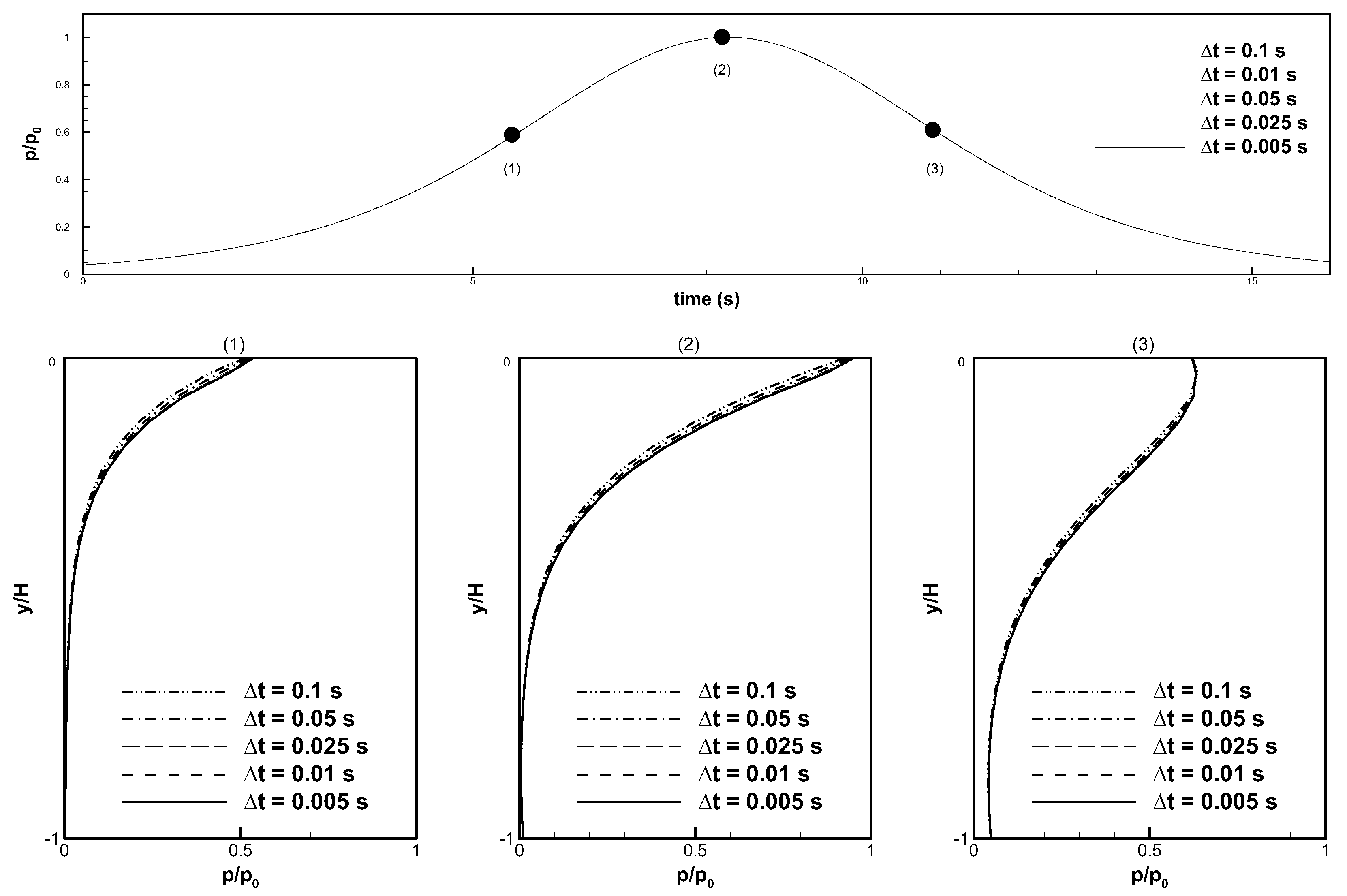
5.1. Convergence Study

First, a convergence test of the model was performed to determine a suitable time step. The soil permeability coefficient of the seabed was $k=1.0\times {10}^{-3}\mathrm{m}/\mathrm{s}$, Young’s modulus was $E=1.0\times {10}^4$ kPa, and the other parameters were as listed previously. The calculation time interval $\Delta t=0.1$ s, 0.05 s, 0.025 s, 0.01 s, and 0005 s. Total simulation time is 30 s, and the mesh size is $0.368\mathrm{m}\times 0.368\mathrm{m}$. Figure 8 shows, for different time steps, the excess pore water pressure change at a fixed place on the seabed as a solitary wave passed by. The upper panel illustrates the solitary wave height at that location, whereas the lower panel displays the vertical profile of the excess pore-water pressure on the seabed at three time points. Figure 8 indicates that the calculation results converged. The difference between the pressure obtained for $\Delta t=0.01$ s and $\Delta t=0.005$ s was extremely small. Considering calculation efficiency, this study adopted $\Delta t=0.01$ s as the time step in subsequent numerical simulations. The computing time of the subsequent cases is about 15 min on a personal computer with an Intel Core i5 3.8 GHz CPU.

5.2. Effects of Permeability

The Young’s modulus at the seabed was set to $E=2.5\times {10}^3$ kPa, and three permeability coefficients were employed: $k=2.5\times {10}^{-1}$ m/s, $2.5\times {10}^{-2}$ m/s, and $2.5\times {10}^{-3}$ m/s. Figure 9 shows the contours of nondimensional excess pore-water pressure when the wave crest passed $x=0$ for seabed with different permeability coefficients. When the permeability coefficient was small, the pore water pressure transmission speed was low. As the depth was increased, the pore pressure isopleth skewed toward the back of the solitary wave’s crest. When the permeability coefficient was large ($k=2.5\times {10}^{-1}$ m/s), the pore pressure isopleth was almost symmetrical. Figure 10 illustrates the vertical pressure distribution over time at a fixed location and for various permeability parameters. When the permeability coefficient was small, pore water pressure was transmitted less easily, and the vertical pressure gradient was more pronounced.

5.3. Effects of Young’s Modulus

The Young’s modulus of loose and dense seabed are generally $E\simeq O\left({10}^3\right)\sim O\left({10}^4\right)$ kPa and $E\simeq O\left({10}^6\right)\sim O\left({10}^7\right)$ kPa, respectively. To determine the influence of Young’s modulus on the excess pore-water pressure caused by a solitary wave, in the following cases the Young’s modulus at the seabed was set to be $E=1.0\times {10}^4$ kPa or $1.0\times {10}^7$ kPa, the permeability parameter as $k=1.0\times {10}^{-4}$ m/s, and the amplitude of the solitary wave as $a/h=0.5$. The rest of the parameters were the same as in Section 5.2. Figure 11 displays the contours of the nondimensional excess pore-water pressure when the solitary wave’s crest passed $x=0$ for different Young’s moduli. Figure 12 illustrates the vertical profile of excess pore-water pressure at the same location at different times for two types of soil. When the permeability coefficients were the same, the more dense soil was displaced more easily and more readily transmitted the pore-water pressure to the depths of the seabed. Therefore, the excess pore-water pressure gradient of the dense soil was smaller than that of the loose soil.

6. Seepage Force on Pipeline Induced by Solitary Waves

This section discusses the solitary-wave-induced seepage force on a pipeline buried under soils of different Young’s moduli and permeability coefficients. The seepage force herein refers to the resultant force on the pipeline induced by excess pore-water pressure. A series of tests on different wave amplitudes showed that the seepage force varies nearly linearly with the wave amplitude. In order to shorten the article, the effect of wave amplitude is not discussed.

The simulation conditions were as follows: solitary wave amplitude $a=1.0$ m, water depth $h=3.0$ m, pipeline diameter $D=1.0$ m, burial depth $b=1.0$ m, Poisson ratio $\mu =0.33$, and time interval $\Delta t=0.01$ s. To investigate the effects of Young’s modulus and permeability coefficient of the soil on seepage force, five Young’s modulus values were employed (i.e., $E=1.0\times {10}^3$, $1.0\times {10}^4$, $1.0\times {10}^5$, $1.0\times {10}^6$, and $1.0\times {10}^7$ kPa) and seven permeability coefficients were used (i.e., $k=1.0\times {10}^{-3}$, $5.0\times {10}^{-4}$, $1.0\times {10}^{-4}$, $5.0\times {10}^{-5}$, $1.0\times {10}^{-5}$, $5.0\times {10}^{-6}$, and $1.0\times {10}^{-6}$ m/s) in simulations. A total of 35 calculations were performed.

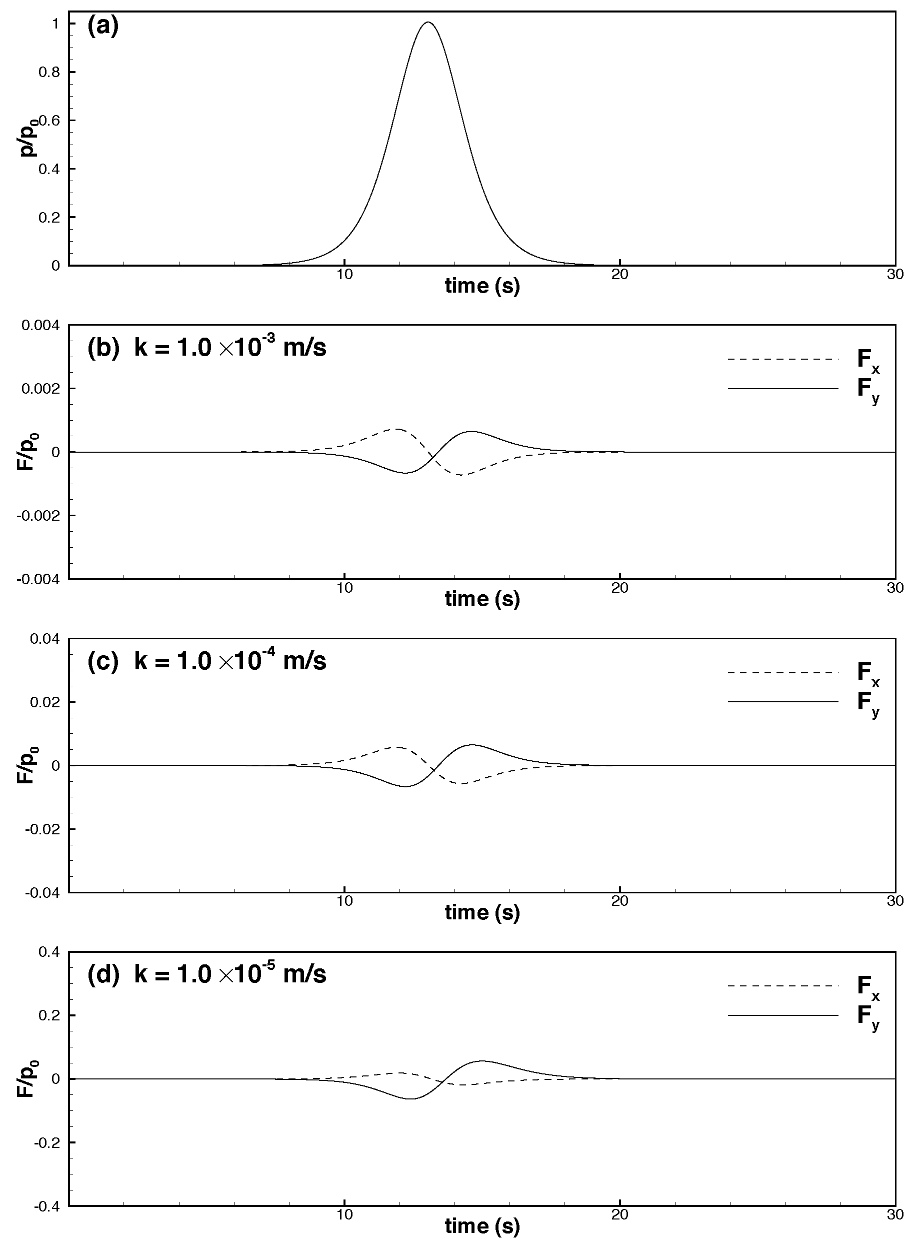
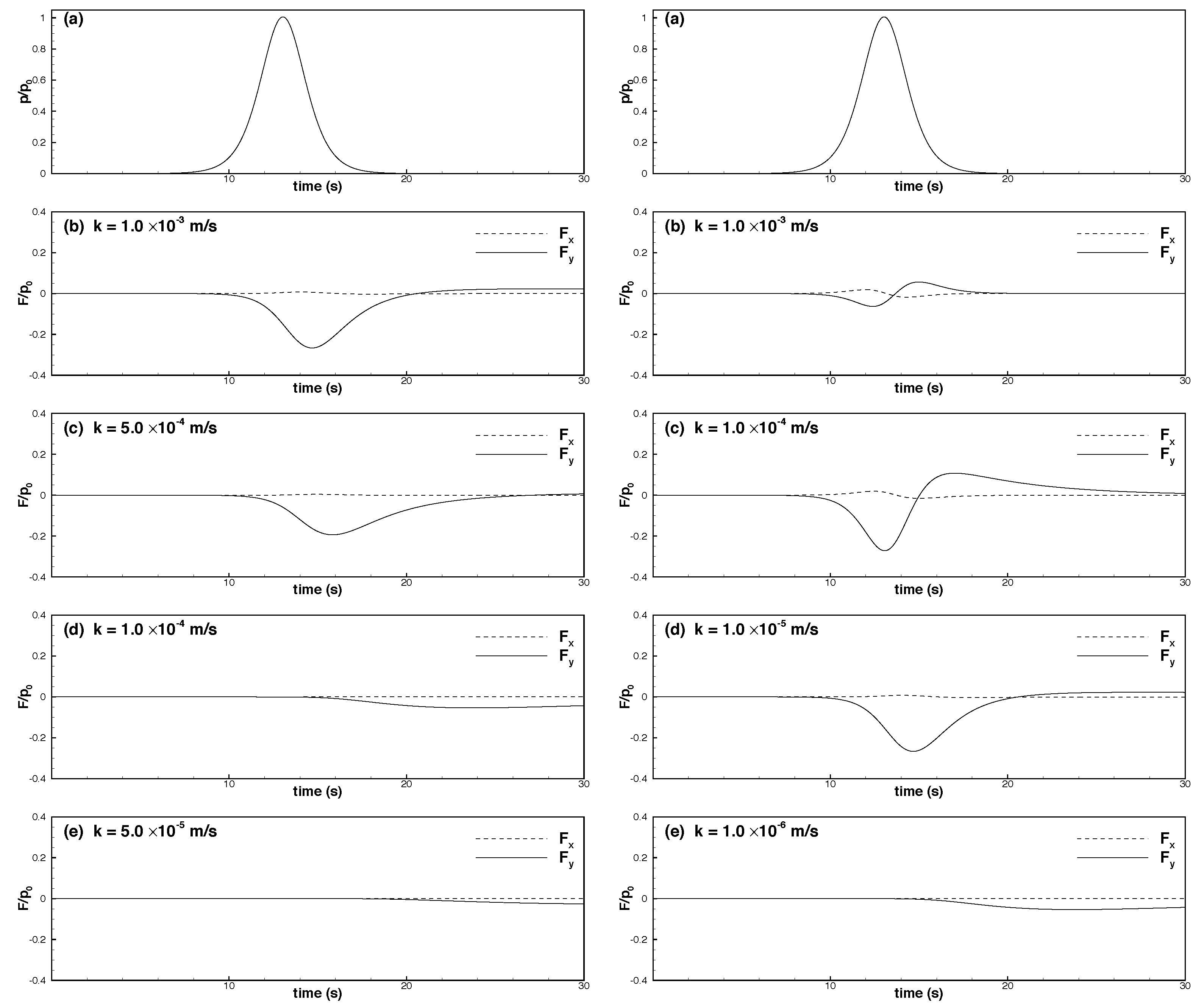
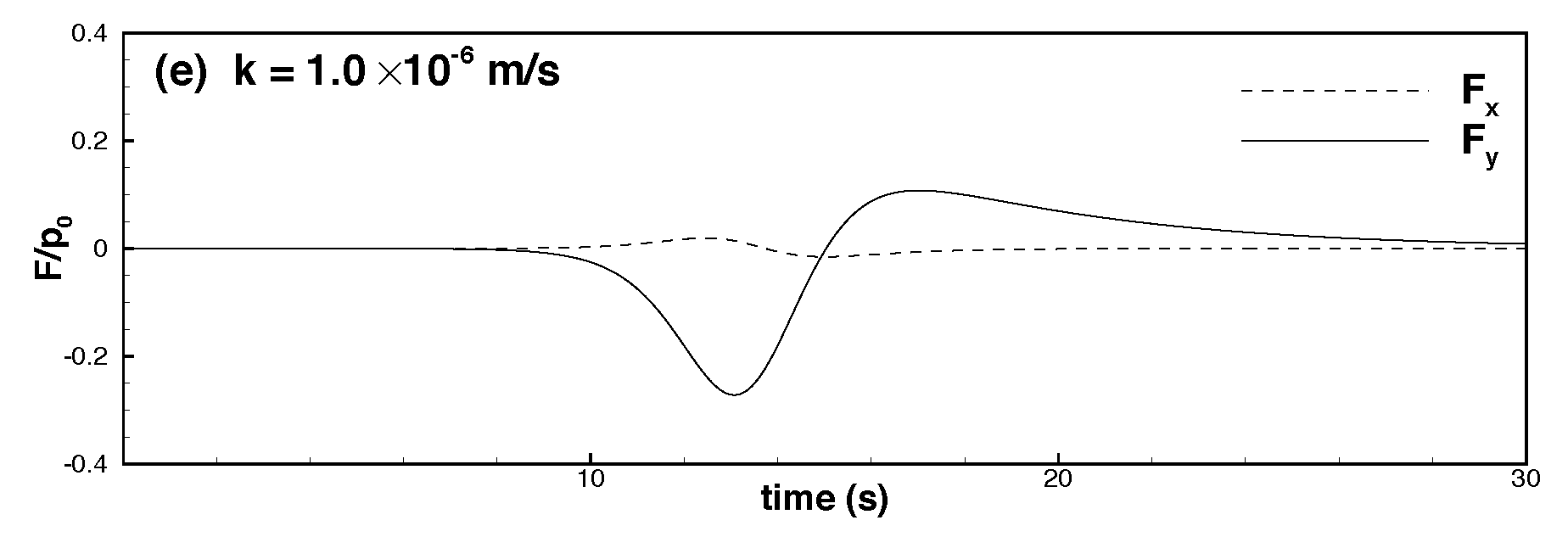
6.1. Effects of Permeability

The influence of the permeability coefficient of the seabed soil on seepage force on the pipeline was determined for a certain Young’s modulus. In the first simulation, the Young’s modulus was set to $1.0\times {10}^3$ kPa, representing loose, sandy soil. The left half of Figure 13 illustrates the change over time in the solitary-wave-induced seepage force on the pipeline in seabed with various permeability coefficients and the corresponding seabed surface water pressure changes. The seepage force on the pipeline is calculated by integrating the excess pore pressure along the surface of the pipeline. $F_x$ and $F_y$ are the horizontal and vertical components of the seepage force, respectively. The results demonstrated that in loose soil with high permeability coefficient ($k=5.0\times {10}^{-4}\sim {10}^{-3}$ m/s), a downward seepage force was exerted on the pipeline when the solitary wave approached, with the force in the horizontal direction being relatively small. The downward seepage force reached its maximum after the solitary wave’s crest has passed and decreased as the solitary wave left. By contrast, in loose soil with low permeability coefficient ($k\le {10}^{-4}$ m/s), the pipeline seepage force was lower, although the same trend of increasing and then decreasing downward seepage force was observed. However, the reaction time was delayed compared with the action of the solitary wave. When the permeability coefficient was small, the pore water flow was slow, causing a greater delay as the permeability coefficient was decreased.

In the second simulation case, the Young’s modulus was set to $E=1.0\times {10}^5$ kPa, representing medium-dense soil. The seepage force induced by the solitary wave for various permeability coefficients is illustrated in the right half of Figure 13. When the permeability coefficient was large ($k={10}^{-3}$ m/s), the magnitudes of vertical and horizontal seepage forces were equal. When the permeability coefficient was small ($k={10}^{-4}$∼${10}^{-5}$ m/s), the downward seepage force was substantially higher, and the time delay of occurrence increased as k was reduced, as for the loose sand. However, when the permeability coefficient was rather low ($k={10}^{-6}$ m/s), the vertical seepage force was low and there was a long-time delay.

In the third simulation case, the Young’s modulus was set to $1.0\times {10}^7$ kPa, representing dense soil. The calculation results are displayed in Figure 14. Because pore water pressure is transmitted more quickly in dense soil, when the permeability coefficient was large ($k={10}^{-3}$∼${10}^{-4}$ m/s), the gradient of excess pore water pressure in the seabed was small; consequently, the seepage force on the pipeline was also small. As the permeability coefficient was reduced, the vertical gradient of the excess pore water pressure increased, so the seepage force in the vertical direction increased.

In summary, this study learned that in looser soil, a larger permeability coefficient resulted in a higher vertical seepage force, whereas in more dense soil, a smaller permeability coefficient resulted in a higher vertical seepage force. Compared with the vertical seepage force, the horizontal seepage force was low in both cases.

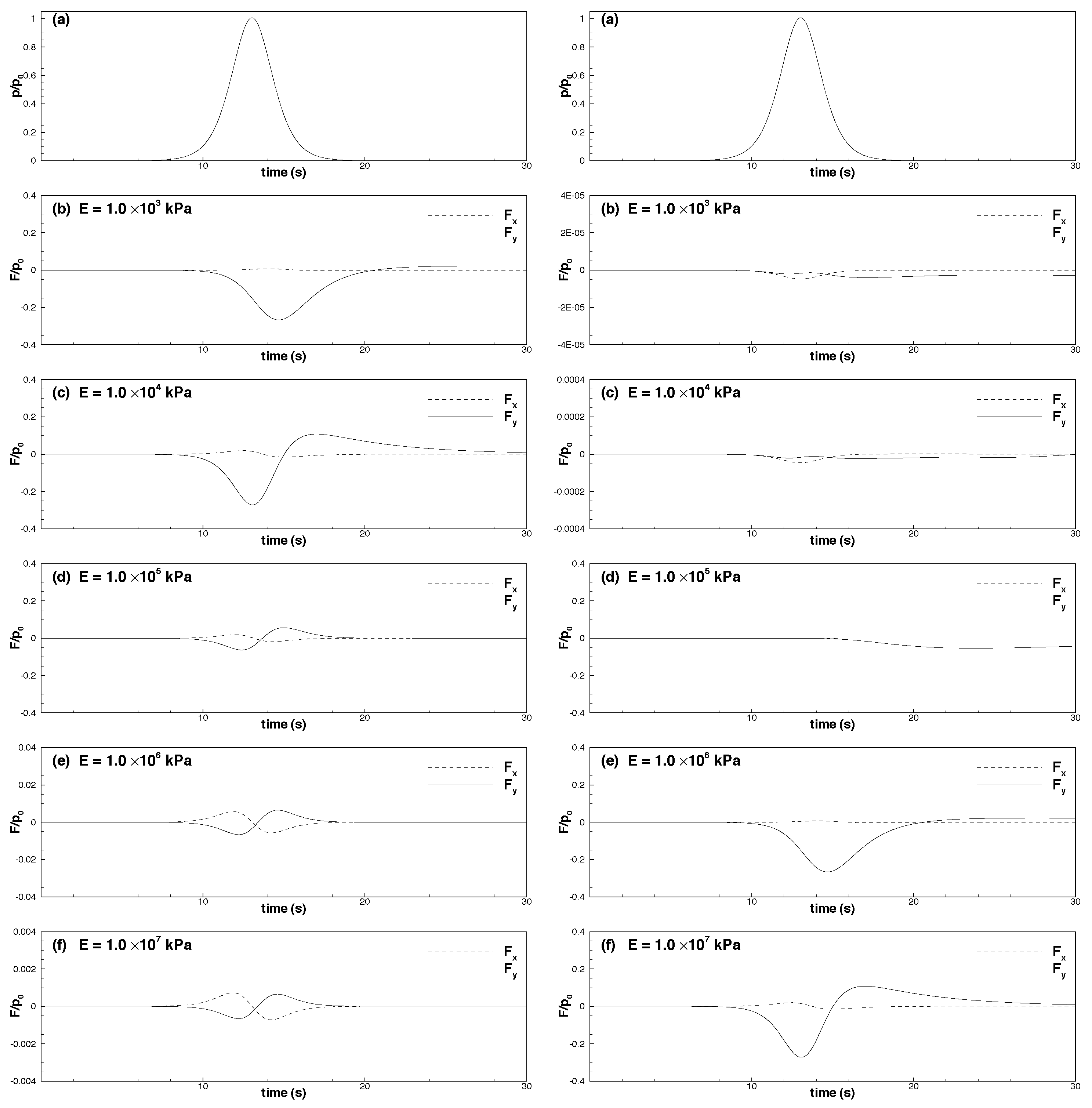
6.2. Effects of Young’s Modulus

The influence of the Young’s modulus of the seabed soil on pipeline seepage force was next determined for various permeability coefficients. Figure 15 illustrate the seepage force over time under different Young’s moduli ($E={10}^3$∼${10}^7$ kPa) for a permeability coefficient of $k={10}^{-3}$ m/s and ${10}^{-4}$ m/s, respectively. When the permeability coefficient was large (the left half of Figure 15), because the permeability of the pore-water flow was stronger, the pore water pressure gradient was more pronounced in the loose soil, resulting in a high vertical seepage force. By contrast, in the soil with smaller permeability coefficient (the right half of Figure 15), because the pore water flow permeability was low, the more dense soil enabled faster pore water pressure transmission and generated a more pronounced pressure gradient, thereby generating a higher vertical seepage force.

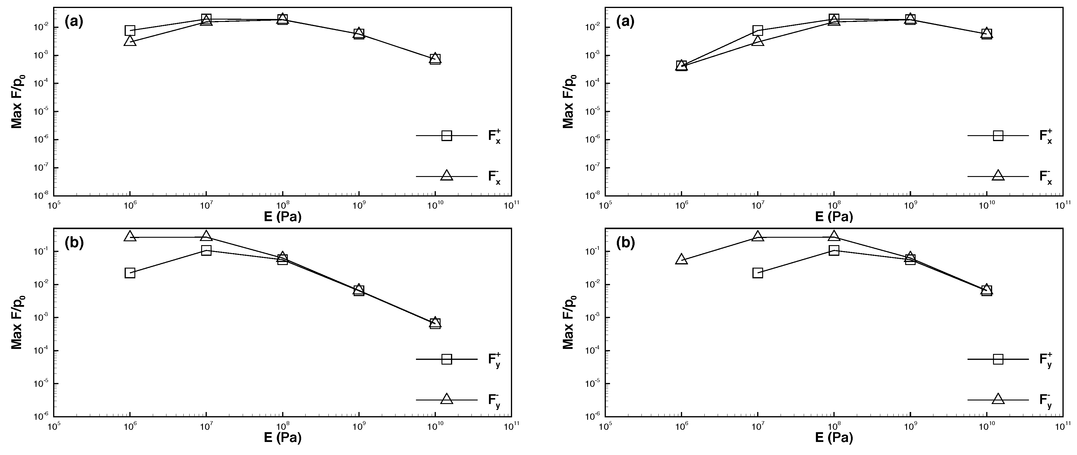
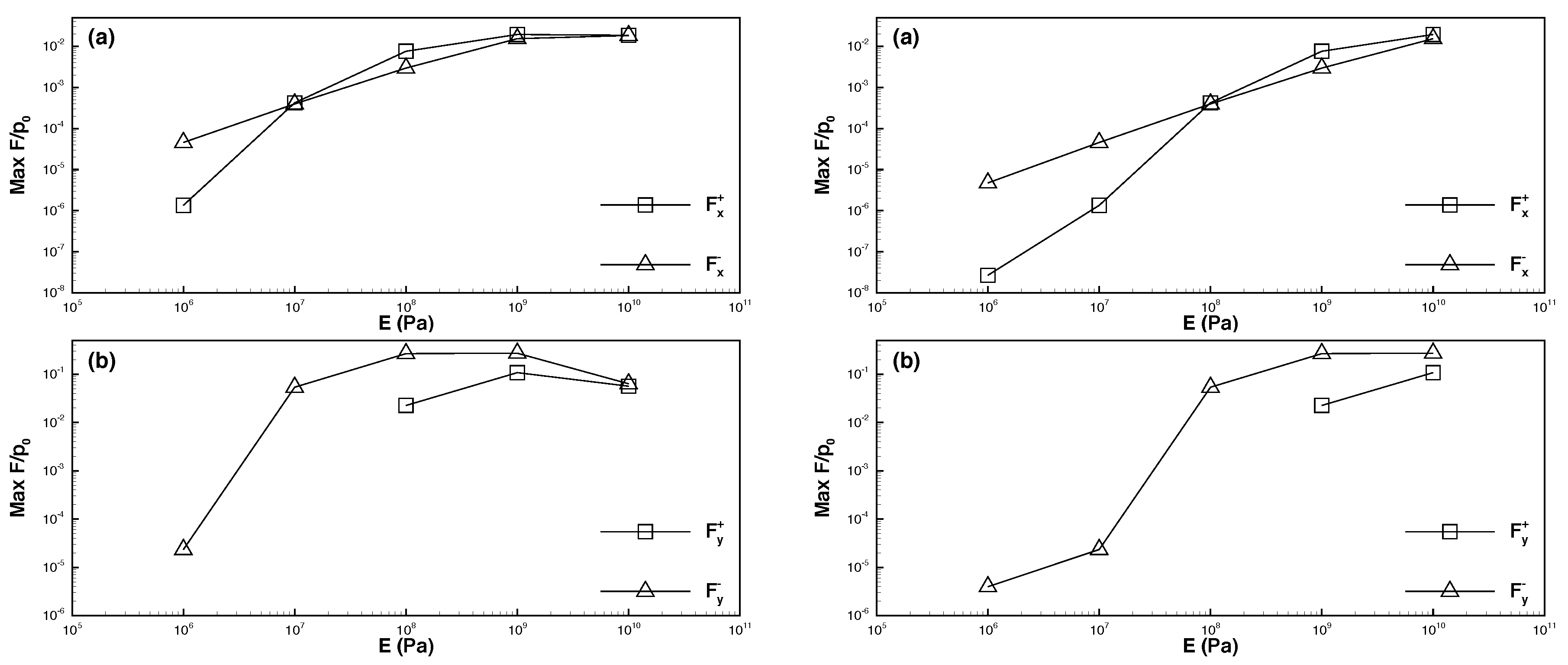
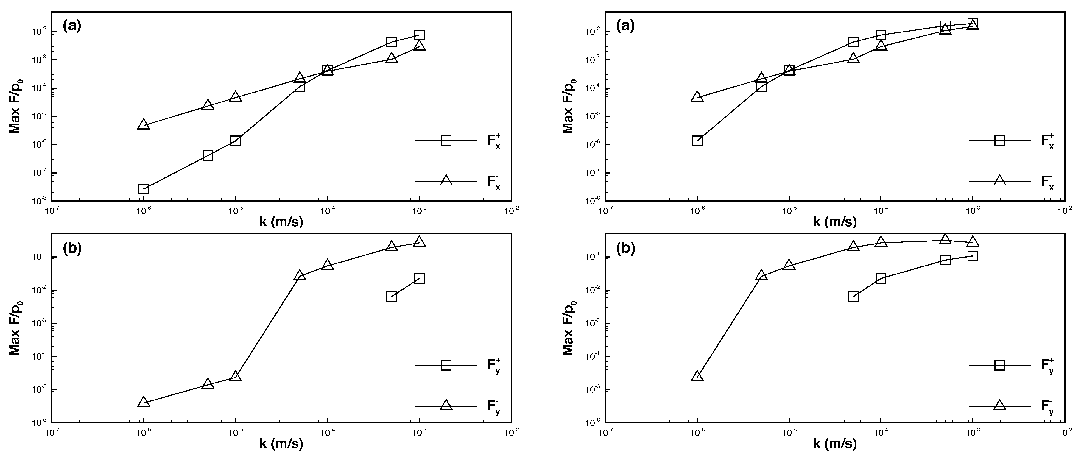
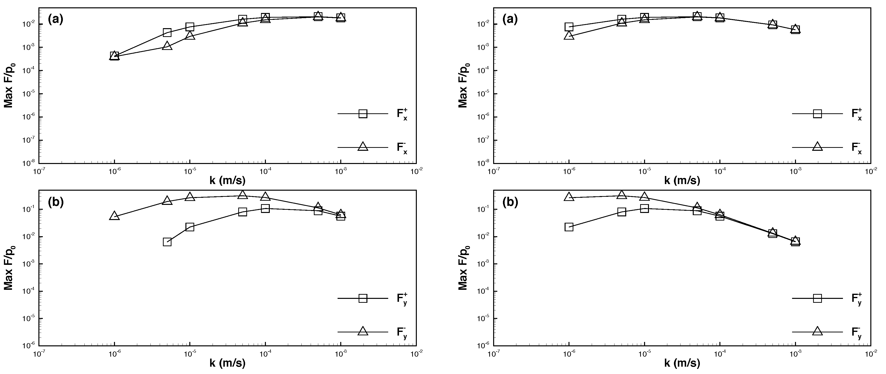
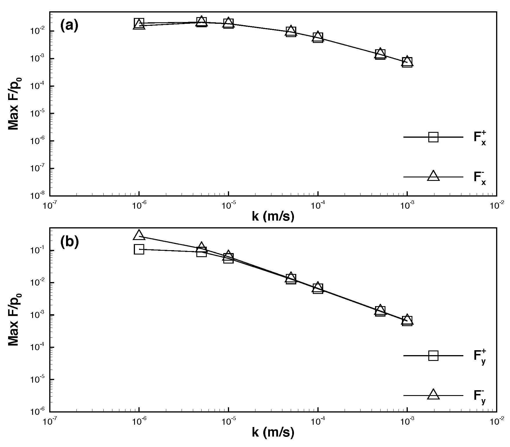
6.3. Maximum Seepage Forces

The relationships between maximum seepage force in different directions and the parameters employed above are illustrated in Figure 16, Figure 17, Figure 18, Figure 19 and Figure 20, where $F_x^{+}$ and $F_x^{-}$ denote the maximum rightward and leftward horizontal forces, respectively, whereas $F_y^{+}$ and $F_y^{-}$ are the maximum upward and downward vertical forces, respectively.

First, under certain permeability coefficients (i.e., $k={10}^{-3}$, ${10}^{-4}$, ${10}^{-5}$, and ${10}^{-6}$ m/s), the relationship between the maximum seepage force and Young’s modulus was determined (Figure 16 and Figure 17). The figures reveal that the trends in horizontal and vertical maximum seepage force were similar, but the vertical component of the force was one order of magnitude higher than the horizontal component. Because the vertical downward component was the dominant component, this study focused on the downward seepage force when discussing the trend of change. When the permeability coefficient was large (e.g., $k={10}^{-3}$ m/s), the maximum seepage force decreased as the Young’s modulus was increased. When $k={10}^{-4}$ m/s, the maximum seepage force first increased and then decreased as the Young’s modulus was increased. When the permeability coefficient was small (e.g., $k={10}^{-5}$ and ${10}^{-6}$ m/s), the maximum seepage force increased as the Young’s modulus was increased.

Next, under specific Young’s moduli (i.e., $E={10}^3$, ${10}^4$, ${10}^5$, ${10}^6$, and ${10}^7$ kPa), the relationship between the maximum seepage force on the pipeline and the permeability coefficient was determined (Figure 18, Figure 19 and Figure 20). In looser soil (i.e., $E={10}^3$∼${10}^4$ kPa), the maximum seepage force increased as the permeability coefficient was increased. In medium-dense soil (i.e., $E={10}^5$ kPa), the maximum seepage force first increased and then decreased as the permeability coefficient was increased. In dense soil (i.e., $E={10}^6$∼${10}^7$ kPa), the maximum downward seepage force decreased as the permeability coefficient was increased.

7. Conclusions

This study employed Biot’s consolidation theory and used the finite-element method to construct a model for calculating the stress and pore water pressure of a two-dimensional elastic medium. The model was used to analyze the pore water pressure transmitted as a solitary wave passes over poroelastic seabed as well as the resultant seepage force exerted on a pipeline buried in the soil. This study investigated the influence of the Young’s modulus of the seabed and permeability coefficient on the force exerted on a pipeline by systematically simulating the variation in seepage force under different parameter conditions.

The soil of the seabed is assumed to be homogeneous with a flat mudline. The pore water within the seabed is assumed to be incompressible. The flow above the seabed is generated only by the solitary waves. The assumptions of the soil are common, but the pore water may be compressible if there is air in it. In the ocean, in addition to surface waves, there are also tides and currents. Future studies may include the compressibility of the pore water and the effects of currents, and also discuss soil liquefaction and the deformation of seabed when a solitary wave is transmitted to the nearshore and uprushes.

Several conclusions were drawn from the findings:

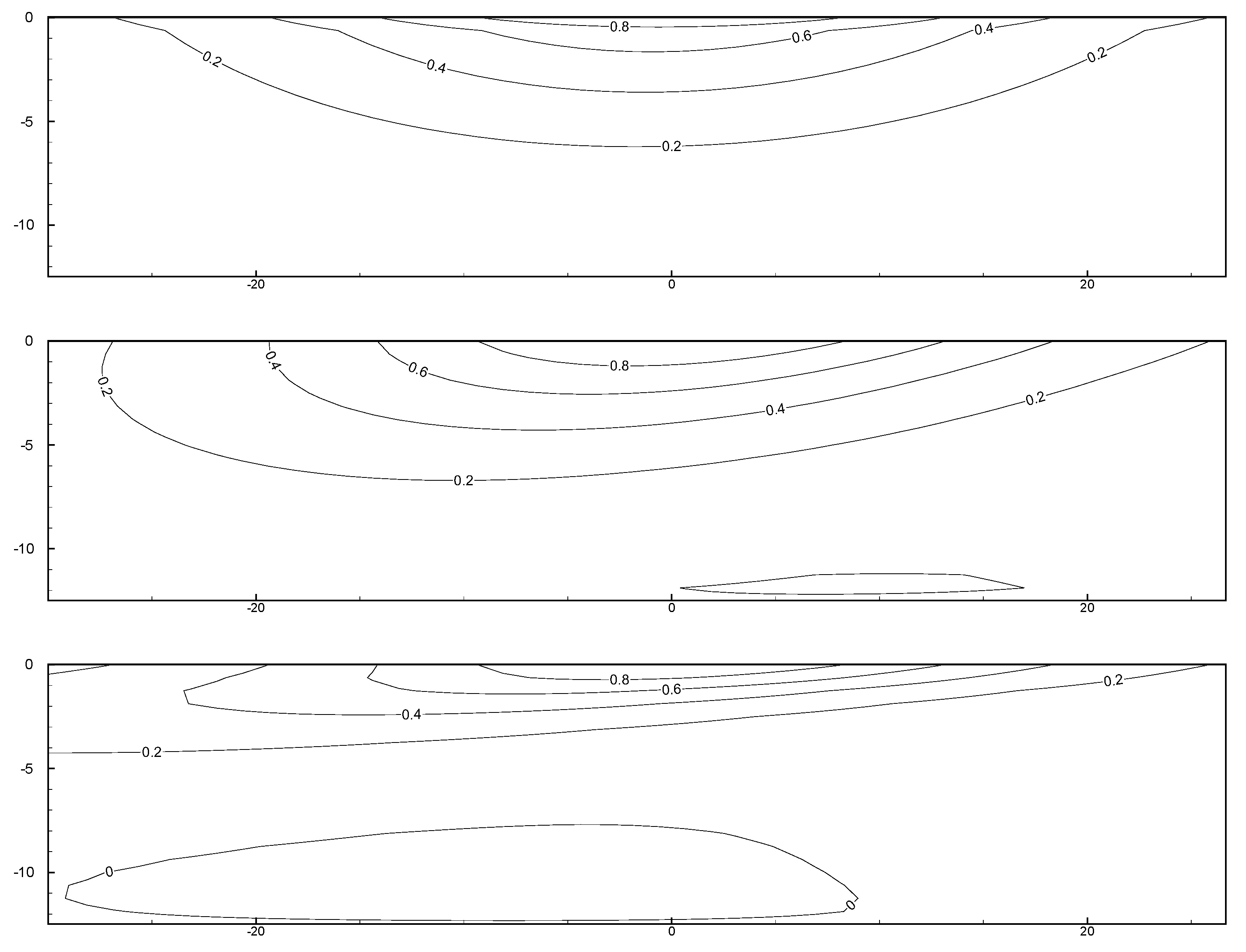
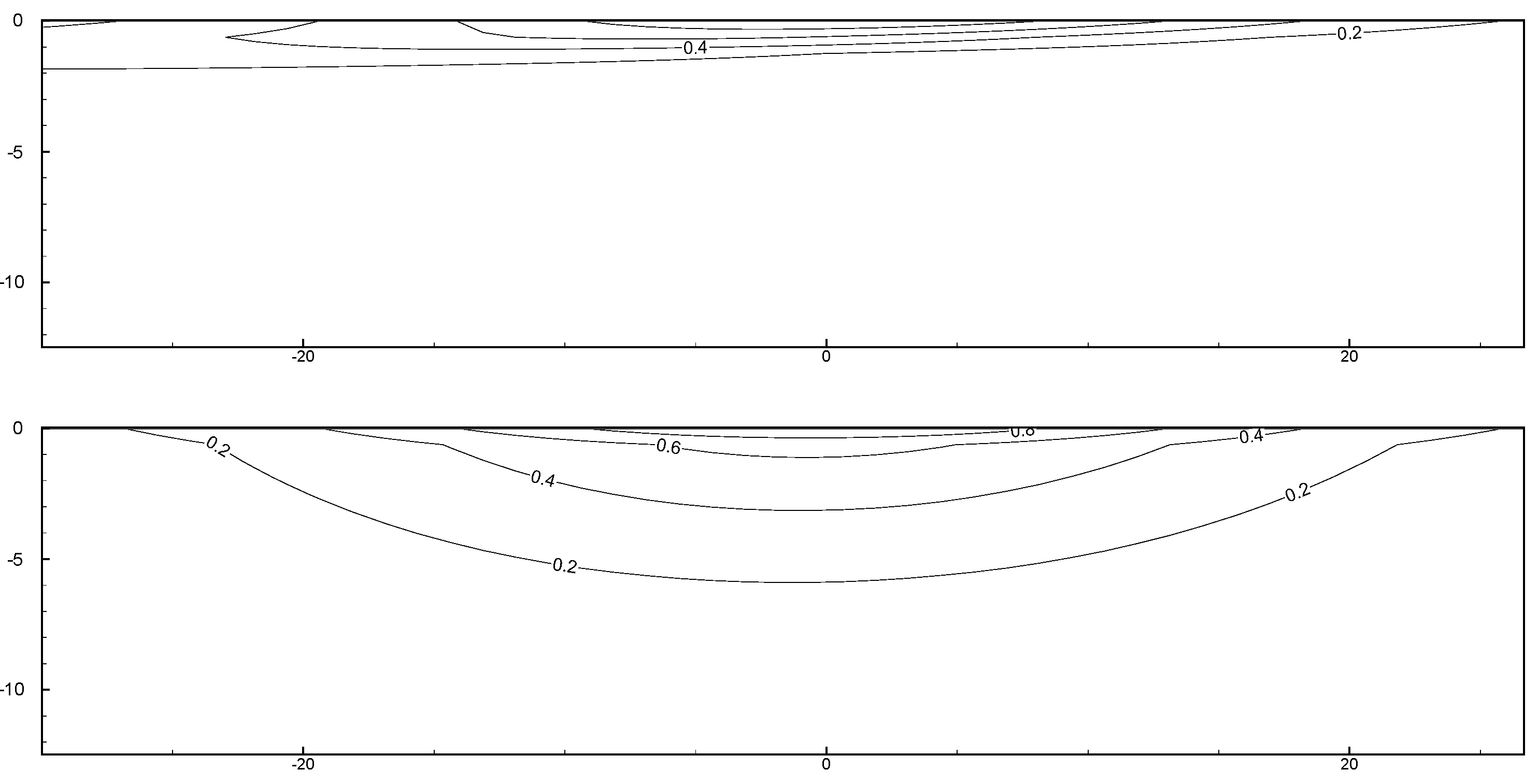
• A lower permeability coefficient increased the difficulty in the propagation of water pressure, thus increasing the vertical gradient of excess pore water pressure. Additionally, when excess pore water pressure dissipated more slowly, the corresponding isoline shifted behind the peak of the solitary wave as the depth increased, indicating an asymmetrical spatial distribution.
• When the permeability coefficient was constant, dense seabed soils were more likely to be displaced, thus enabling the dissipation of pore water pressure into the depths of the seabed. Hence, the gradient of excess pore water pressure associated with dense seabed soils was lower than that of excess pore water pressure associated with loose seabed soils.
• Most of the seepage force exerted on pipelines embedded in loose seabed soils was vertical:
  • When the permeability coefficient was higher and the solitary wave amplitude increased, the maximum downward vertical force ($F_y^{-}$) increased considerably, whereas the upward vertical force ($F_y^{+}$) decreased slightly. The horizontal force was weaker than the vertical force by one order of magnitude. Moreover, the maximum leftward and rightward horizontal forces ($F_x^{-}$ and $F_x^{+}$) increased with the solitary wave amplitude.
  • When the permeability coefficient was lower and the solitary wave amplitude increased, the maximum downward and upward vertical forces decreased, and the upward force was weaker than the downward force by one order of magnitude. Furthermore, the horizontal force was weaker than the vertical force by nearly two orders of magnitude. As the solitary wave amplitude increased, the maximum rightward horizontal force increased, whereas the maximum leftward horizontal force decreased.
• The force exerted on a pipeline embedded in dense seabed soils was weaker than that exerted on a pipeline embedded in loose seabed soils. Specifically, if the permeability coefficient was higher, the force exerted on the pipeline in dense seabed soils was weaker than that exerted on the pipeline in loose seabed soils by two to three orders of magnitude (or greater if the coefficient was lower).

References

1. Biot, M.A. General theory of three-dimensional consolidation. J. Appl. Phys. 1941, 12, 155–164. [Google Scholar] [CrossRef]
2. Massel, S.R. Gravity waves propagated over permeable bottom. J. Waterw. Harb. Coast. Eng. 1976, 102, 111–121. [Google Scholar]
3. Madsen, O.S. Wave-induced pore pressures and effective stresses in a porous bed. Géotechnique 1978, 28, 377–393. [Google Scholar] [CrossRef]
4. Yamamoto, T.; Koning, H.L.; Sellmeijer, H.; Van Hijum, E. On the response of a poro-elastic bed to water waves. J. Fluid Mech. 1978, 87, 193–206. [Google Scholar] [CrossRef]
5. Magda, W. Analytical Solution for the Wave-Induced Excess Pore-Pressure in a Finite-Thickness Seabed Layer. In 24th International Conference on Coastal Engineering; American Society of Civil Engineers: New York, NY, USA, 1994; pp. 3111–3125. [Google Scholar]
6. Magda, W. Wave-induced uplift force acting on a submarine buried pipeline: Finite element formulation and verification of computations. Comput. Geotech. 1996, 19, 47–73. [Google Scholar] [CrossRef]
7. Magda, W. Wave-induced cyclic pore-pressure perturbation effects in hydrodynamic uplift force acting on submarine pipeline buried in seabed sediments. Coast. Eng. 2000, 39, 243–272. [Google Scholar] [CrossRef]
8. Wang, J.G.; Karim, M.R.; Lin, P.Z. Analysis of seabed instability using element free Galerkin method. Ocean Eng. 2007, 34, 247–260. [Google Scholar] [CrossRef]
9. Liu, P.L.F.; Park, Y.; Lara, J.L. Long-wave-induced flows in an unsaturated permeable seabed. J. Fluid Mech. 2007, 586, 323–345. [Google Scholar] [CrossRef]
10. Nakamura, H.; Onishi, R.; Minamide, H. On the Seepage in the Seabed Due to Waves. In Proceedings of 20th Coastal Engineering Conference; Japan Society of Civil Engineers: Tokyo, Japan, 1973; pp. 421–428. (In Japanese) [Google Scholar]
11. McDougal, W.G.; Davidson, S.H.; Monkmeyer, P.L.; Sollitt, C.K. Wave-induced forces on buried pipelines. J. Waterw. Port Coast. Ocean Eng. 1988, 38, 331–336. [Google Scholar] [CrossRef]
12. Sumer, B.M. Flow–structure–seabed interactions in coastal and marine environments. J. Hydraul. Res. 2014, 52, 1–13. [Google Scholar] [CrossRef]
13. Verruijt, A. Elastic Stoage of Aquifers. In Flow through Porous Media; De Wiest, R.J.M., Bear, J., Eds.; Academic Press: New York, NY, USA, 1969; pp. 311–376. [Google Scholar]
14. Boussinesq, J. Théorie des ondes et des remous qui se propagent le long d’un canal rectangulaire horizontal, en communiquant au liquide contenu dans ce canal des vitesses sensiblement pareilles de la surface au fond. J. Math. Pures Appl. 1872, 17, 55–108. [Google Scholar]
15. Smith, I.M.; Griffiths, D.V.; Margetts, L. Programming the Finite Element Method; John Wiley & Sons, Ltd.: Chichester, UK, 2015. [Google Scholar]
16. Gordon, W.J.; Hall, C.A. Construction of curvilinear co-ordinate systems and applications to mesh generation. Int. J. Numer. Methods Eng. 1973, 7, 461–477. [Google Scholar] [CrossRef]
17. Schiffman, R.L. Field applications of soil consolidation, time-dependent loading and variable permeability. Highw. Res. Board Bull. 1960, 248, 25. [Google Scholar]
Figure 1. Schematic diagram of research area.
Jmse 08 00324 g001
Figure 2. Boundary conditions of the soil consolidation problem.
Jmse 08 00324 g002
Figure 3. Nodal points of rectangular element.
Jmse 08 00324 g003
Figure 4. Mesh system of the calculation with a pipeline (400 non-rectangular elements with in the rectangle zone of the pipeline nearest proximity, and 3300 square elements outside the rectangle zone).
Jmse 08 00324 g004
Figure 5. Mesh system of one-dimensional soil consolidation problem.
Jmse 08 00324 g005
Figure 6. Surface loading of one-dimensional consolidation problem.
Jmse 08 00324 g006
Figure 7. Results of the excess pore-water pressure in the one-dimensional consolidation problem.
Jmse 08 00324 g007
Figure 8. Distribution of excess pore-water pressure computed using different time steps.
Jmse 08 00324 g008
Figure 9. Contours of dimensionless excess pore-water pressure for different permeability coefficients (from top to bottom: k = 2.5 × 10 1 , 2.5 × 10 2 , 2.5 × 10 3 m / s ); Young’s modulus E = 2.5 × 10 3 kPa.
Jmse 08 00324 g009
Figure 10. Distribution of excess pore-water pressure for Young’s modulus E = 2.5 × 10 3 kPa, and various permeability coefficients: ——–, k = 2.5 × 10 1 m / s ; , k = 2.5 × 10 2 m / s ; · , k = 2.5 × 10 3 m / s .
Jmse 08 00324 g010
Figure 11. Contours of dimensionless excess pore-water pressure for different value of Young’s modulus (From top to bottom, E = 1.0 × 10 4 and 1.0 × 10 7 kPa ); k = 1.0 × 10 4 m/s.
Jmse 08 00324 g011
Figure 12. Distribution of excess pore-water pressure for permeability coefficient k = 1.0 × 10 4 m/s and various Young’s modulus: ——–, E = 1.0 × 10 4 kPa; , E = 1.0 × 10 7 kPa.
Jmse 08 00324 g012
Figure 13. Time evolution of seepage force exerted on the pipeline at various k values and left: E = 1.0 × 10 3 kPa ; right: E = 1.0 × 10 5 kPa . (a) Dynamic pressure at the seabed above the pipeline; (be) horizontal and vertical components of seepage force at different k value.
Jmse 08 00324 g013
Figure 14. Time evolution of seepage force exerted on the pipeline at E = 1.0 × 10 7 kPa and various k values. (a) Dynamic pressure at the seabed above the pipeline; (be) horizontal and vertical components of seepage force.
Jmse 08 00324 g014aJmse 08 00324 g014b
Figure 15. Time evolution of seepage force exerted on the pipeline at various E values and left: k = 1.0 × 10 3 m / s ; right: k = 1.0 × 10 6 m / s . (a) Dynamic pressure at the seabed above the pipeline; (bf) horizontal and vertical components of seepage force at different E value.
Jmse 08 00324 g015
Figure 16. Maximum force on the pipeline in relation to Young’s modulus; left: k = 1.0 × 10 3 m / s ; right: k = 1.0 × 10 4 m / s . (a) Horizontal component; (b) vertical component.
Jmse 08 00324 g016
Figure 17. Maximum force on the pipeline in relation to Young’s modulus; left: k = 1.0 × 10 5 m / s ; right: k = 1.0 × 10 6 m / s . (a) Horizontal component; (b) vertical component.
Jmse 08 00324 g017
Figure 18. Maximum force on the pipeline in relation to soil permeability; left: E = 1.0 × 10 3 kPa ; right: E = 1.0 × 10 4 kPa . (a) Horizontal component; (b) vertical component.
Jmse 08 00324 g018
Figure 19. Maximum force on the pipeline in relation to soil permeability; left: E = 1.0 × 10 5 kPa ; right: E = 1.0 × 10 6 kPa . (a) Horizontal component; (b) vertical component.
Jmse 08 00324 g019
Figure 20. Maximum force on the pipeline in relation to soil permeability; E = 1.0 × 10 7 kPa . (a) Horizontal component; (b) vertical component.
Jmse 08 00324 g020