Statistical Modeling of Bilge Water Discharge from Ships During Normal Operation

Abstract

This study estimated the amount of bilge water spilled from ships during normal operation and identified the contributing factors of the discharge by building a statistical model. To build the statistical model, we collected as much information as possible about the amount of bilge water in ships, then used the collected information to formulate a probability distribution of the discharge amount according to Bayesian statistics, and determined the parameters included in the model by applying a Markov Chain Monte Carlo method. The analysis of those parameters shows that the integrated bilge treatment system (IBTS) primarily contributes to reductions in the discharge amount, and that the container-type ship is involved with especially large discharge amounts.

1. Introduction

Normal maritime operations are one of the sources of hydrocarbon release into the ocean. Liquid, including hydrocarbons, is discharged through the washing of ballast and oil tanks. Bilge water (a mixture of water and oil accumulated in the bottom plate of a vessel, which includes a high concentration of organic hydrocarbons) is discharged into the marine environment for a number of reasons. Such discharge from vessels during normal operations is predicted to be a major source of hydrocarbon release into the ocean, along with runoff from rivers and sewage [1]. Bilge water shares a similarity with ballast water, as both are discharged from ships, then unfavorably influence the marine environment. A recent status of treating ballast water was reported by the authors of [2]. This paper presents a method for quantifying the amount of bilge water discharge in order to mitigate marine pollutions due to the normal ship operations.

Oil spills due to maritime accidents devastate the marine environment, especially if the spilled oil drifts on the surface of the sea and eventually arrives at coasts adjacent to the accident site. This marine environmental pollution attracts much attention, because the amount of oil spilled per unit time is extremely large. Meanwhile, the amount of discharge during normal operations per unit time is small. However, unlike oil spills due to maritime accidents, bilge water discharge occurs constantly from numerous vessels [3].

Recently, the United States Environmental Protection Agency (EPA) strengthened requirements for polluted liquid discharge on all commercial vessels greater than 79 feet in length under normal operations [4]. These vessels need to meet several requirements of the vessel general permit (VGP) when they enter within three nautical miles of the United States coastline or inland waters. This enhancement of the regulation suggests that more attention ought to be paid to chronic discharge, such as bilge water discharge, as well as to oil spillage due to maritime accidents.

Several other regulations have been imposed to prevent the marine environment from pollution owing to normal maritime operations. For instance, to reduce petroleum hydrocarbon input to the ocean, the 1978 Protocol of the International Convention for the Prevention of the Pollution from Ships (MARPOL 73/78) was implemented, first in the United States in 1981, and then worldwide in 1983. This regulation mandates the installation of improved ballast tanks to prevent liquids, including hydrocarbons, from leaking into the ocean. These efforts have reduced pollution by petroleum oil. Recently, the International Maritime Organization (IMO) discussed the promotion of the Integrated Bilge Water Treatment System (IBTS), which is able to separately process oily water and clean water to reduce bilge water production and to reuse oily sludge as fuels.

In order to identify which vessel specifications can be factors in bilge water discharge, this study attempted to build a statistical model that appropriately expresses the relationship of the vessel specification with discharge amount. The statistical model developed in this study enables us to quantify the bilge water discharge from various ship types. The establishment of such a statistical model provides useful information for refining the structural design of vessels that tend to discharge a relatively large amount of hydrocarbon, and for updating maritime regulations to protect the marine environment from pollution due to hydrocarbon discharge. In particular, the quantification of bilge water and identification of discharge factor can offer optimized usages of the IBTS and efficient eliminations of discharge factor.

In this study, data were collected through a search of the literature on the amount of bilge water discharged from ships during normal operations, together with information about ship type and construction year. The collected data was then used to build a Bayesian statistical model. Bayesian statistics is a powerful methodology for elucidating a relationship between two variables, even if there is only a small amount of information available. The authors of [5] constructed a receptor model to identify air pollution sources based on the Bayesian method. The authors of [6] used the Bayesian approach to assess the ecological risk in Tokyo surface water due to several toxic substances.

The IBTS mentioned above is expected to contribute to reduction in bilge water. Nevertheless, other factors that potentially result in the discharge of bilge water must be considered. The main purpose of this study was to identify other factors through examining the statistical properties of the parameters used in the model. This study hypothesized that a Bayesian statistical model that involves multiple parameters would provide us with a way to identify the other factors. This paper describes how such a model was built and discusses the factors influencing bilge water discharge by interpreting properties of that model.

In the subsequent sections, two statistical models are described: constant and variable discharge probability models. Through a comparison between those two models, this paper demonstrates the importance of considering uncertainties in the data and parameters used for constructing the model, thereby proving the usefulness of the statistical modeling.

2. Data Collection

Published papers and reports [7,8,9,10] were referred to for the data on ship type, ship size, amount of bilge water, and ship construction year (

Table 1. Data collected for building statistical models. “ND” (no data) means that the item was unavailable. In the Integrated Bilge Water Treatment System (IBTS) column, “W/” and “W/O” refer to vessels with and without IBTS, respectively. In the ship type column, PCC and VLCC stand for pure car carrier and very large car carrier, respectively.

No.	IBTS	Size [GT]	Ship Type	Construction Year	Bilge Water Amount $[{\mathrm{m}}^3/\mathrm{day}]$	Discrete Value of Bilge Water Amount	Ref.
1	W/	145635	Tanker	1987	0.0000	0	[7]
2	W/	149407	Tanker	1999	0.0000	0	[7]
3	W/	50890	Bulk	1995	0.0010	0	[7]
4	W/	75637	Container	1997	0.0280	0	[7]
5	W/	75201	ND	ND	0.1753	0	[8]
6	W/	57623	PCC	1998	0.2330	0	[7]
7	W/	ND	Bulk	ND	0.2532	0	[9]
8	W/	ND	Container	ND	0.2532	0	[9]
9	W/	ND	PCC	ND	0.2532	0	[9]
10	W/	55880	PCC	2000	0.2890	0	[7]
11	W/	ND	ND	ND	0.3945	0	[9]
12	W/	97825	ND	ND	0.4148	0	[8]
13	W/O	ND	Bulk	ND	0.4274	0	[9]
14	W/	53822	Container	2003	0.4880	0	[7]
15	W/	27986	Bulk	1999	0.5010	1	[7]
16	W/O	108000	Bulk	1987	0.6720	1	[7]
17	W/O	52214	PCC	1977	0.6790	1	[7]
18	W/	ND	VLCC	ND	0.7562	1	[9]
19	W/O	ND	PCC	ND	0.8219	1	[9]
20	W/O	46047	PCC	1981	0.9770	1	[7]
21	W/	160079	Tanker	2000	1.0000	2	[7]
22	ND	58192	ND	ND	1.1000	2	[10]
23	W/O	ND	ND	ND	1.5123	3	[9]
24	W/O	42145	ND	ND	1.6866	3	[8]
25	ND	79275	ND	ND	1.7000	3	[10]
26	W/O	42145	Container	1986	1.7100	3	[7]
27	W/O	ND	VLCC	ND	1.8411	3	[9]
28	W/O	145635	Tanker	1987	1.8530	3	[7]
29	W/O	102395	Bulk	1985	1.8810	3	[7]
30	W/O	ND	Container	ND	2.8931	5	[8]
31	ND	141881	ND	ND	3.0000	6	[10]
32	W/O	40354	ND	ND	4.0893	8	[8]
33	W/O	40354	Container	1986	4.1460	8	[7]

). In this table, bilge water amount is written in the unit of m³/day, which was converted from unit of m³ per half year used by the authors of [8], and from m³ per month used by the authors of [9].

One may claim that factors of the bilge water discharge can be revealed just by reading the values listed in Table 1. Such a simple analysis may be enough in order to qualitatively evaluate discharge amounts. However, it cannot serve as a reliable way to address the seawater pollution due to two problems. First, bilge water amount data are generally contaminated by errors through measurement and analysis processes. Second, a conclusion from the simple analysis is inapplicable to a prediction of the amount of discharge from many vessels other than the ones listed in Table 1. Statistical modeling is one of the rational methods for resolving these two problems and for maximizing the utility of collected data.

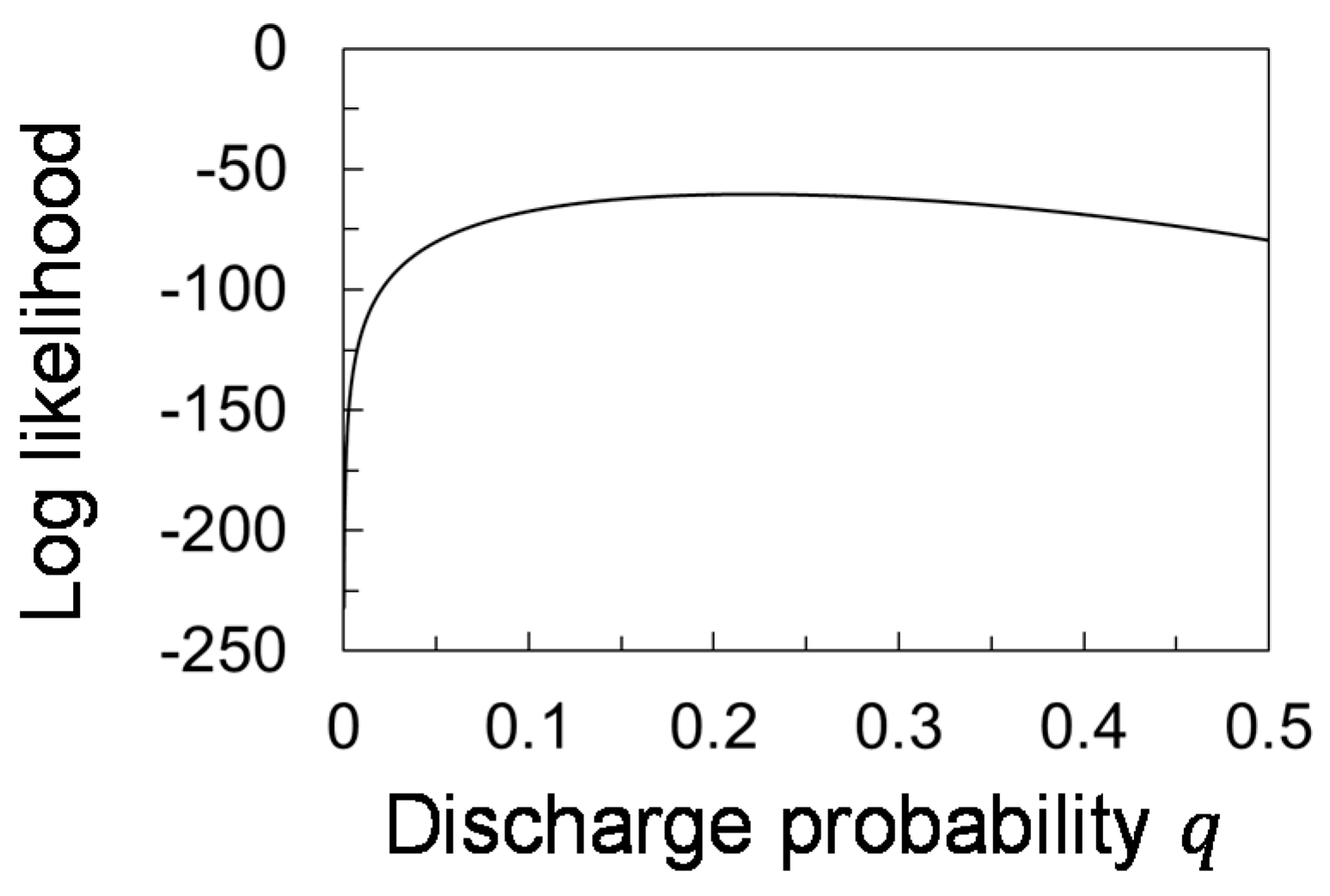
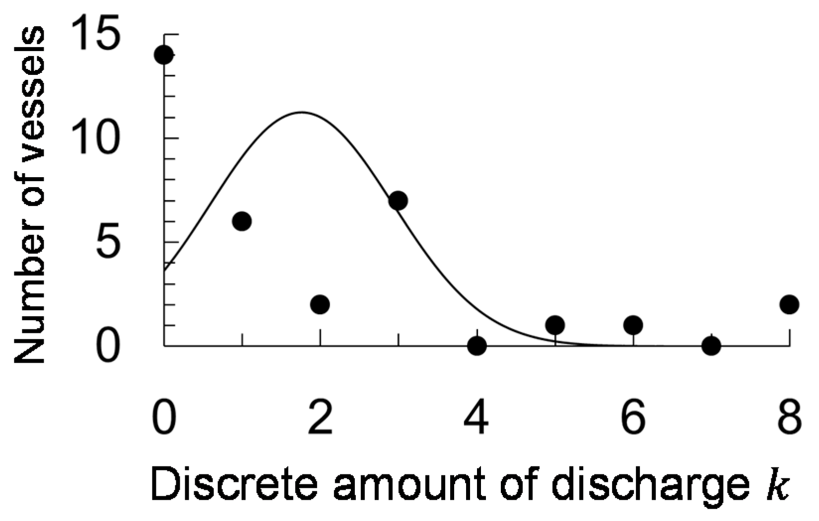
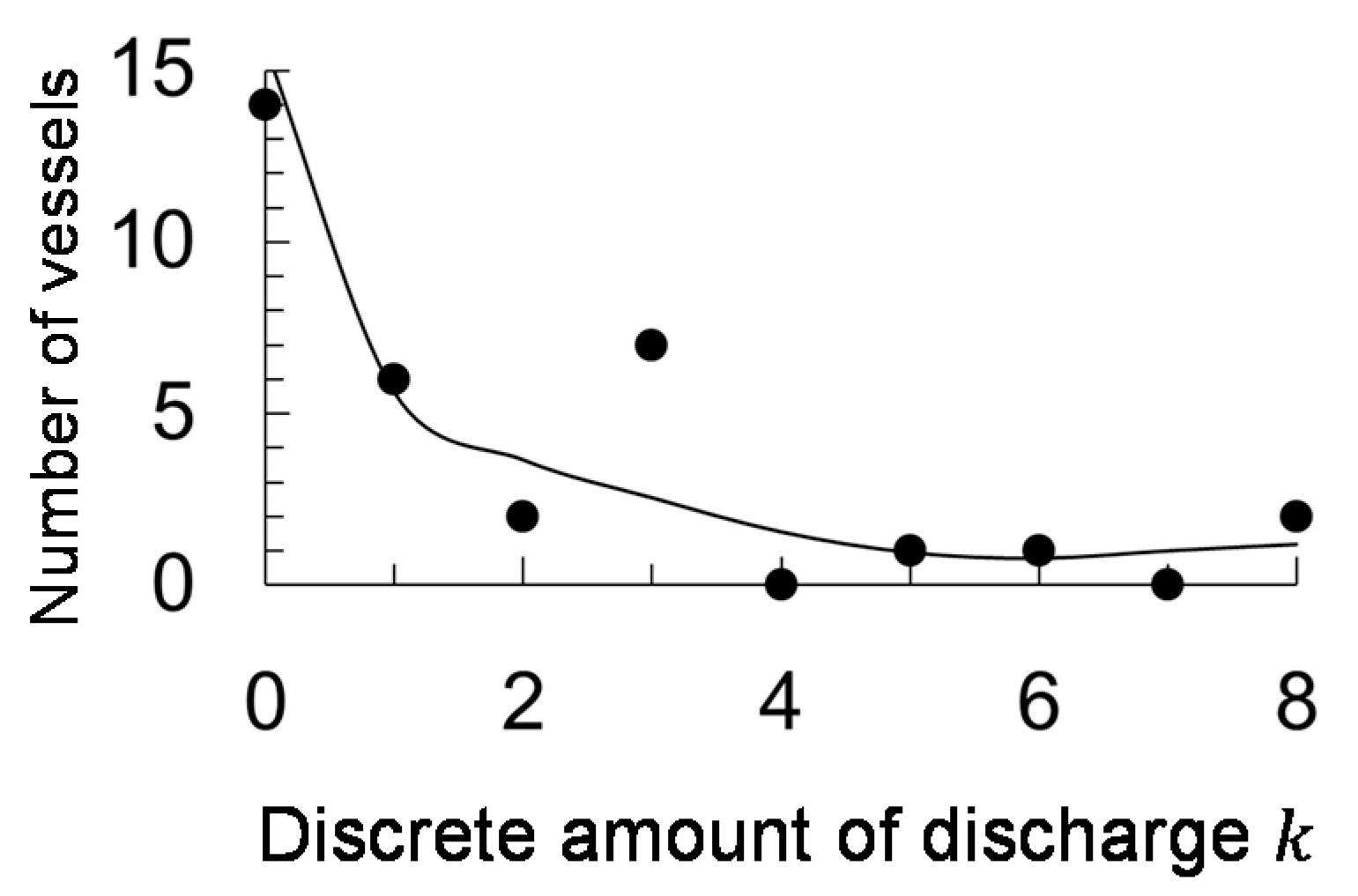
3. Constant Discharge Probability Model

The binomial distribution function was adopted to express the relationship of the response variable, that is, the amount of bilge water, with the explanatory variables, that is, factors contributing to bilge water discharge. The binomial distribution includes a single parameter which determines the occurrence probability of an independent trial, and is thus suitable to simply represent that relationship by regarding the parameter as the occurrence probability of a bilge water discharge event, hereafter referred to as the discharge probability.

The application of the binomial distribution to the present model has the disadvantage of representing the number of event occurrences, which is an integer. Thus, an amount of bilge water, which is originally a continuous value, needs to be converted into a discrete value. In this study, the amount of bilge water ranging from 0 m³/day to 0.5 m³/day was converted to 0 m³/day, that ranging from 0.5 m³/day to 1.0 m³/day was converted to 1 m³/day, and so forth. In this way, the next larger integer was assigned to the amount of bilge water as the amount increased by 0.5 m³/day. With this treatment, a larger amount of discharge was thought of as a larger number of times the trial, that is, the discharge event, occurs. It may be possible to apply the normal distribution function to the present model. The normal distribution function involves two parameters, i.e., mean and variance, both of which have to be specified at the same time for a statistical calculation. By emphasizing the simplicity of the mathematical expression of the binomial distribution function, which makes numerical computations correspondingly simpler, this study applied the binomial distribution.

Denoting the discharge probability mentioned above as $\mathrm{q}$, the likelihood, which measures the extent to which a specification of the parameter reproduces the observation, is expressed as,

$$\mathrm{L}\left(q\right)={\displaystyle \prod }_{i=1}^N\left(\begin{array}{c}{N}_{\mathrm{d}}\\ k\end{array}\right)q^k{\left(1-q\right)}^{N_{\mathrm{d}}-k}$$

(1)

where $\left(\begin{array}{c}{N}_{\mathrm{d}}\\ k\end{array}\right)$ denotes the number of combinations that result from choosing $k$ elements from a set of $N_{\mathrm{d}}$ elements, $N$ indicates the total number of the vessels in Table 1, and $N_{\mathrm{d}}$ represents the maximum discrete value of discharge.

The maximum likelihood method was applied to determine $q$, which, in this model, is constant. Searching for the value of $q$ that maximizes the log-likelihood (Figure 1), $q=0.2218$ was found to provide the best fit of the probability distribution function to the observation.

Comparing the means and variances computed using the observation (Table 1) and applying the maximum likelihood method revealed that, though the mean of the model agrees with the mean of the observation, the model underestimated the variance (

Table 2. Mean and variance of the discrete values of bilge water discharge obtained from observation, the constant discharge probability model, and the variable discharge probability model.

	Mean	Variance
Observation [7,8,9,10]	1.774	5.143
Constant discharge probability model	1.774	1.381
Variable discharge probability model	1.627	5.886

). The expected number of vessels that spill an amount $k$ can be calculated using the formula of the binomial distribution. Comparison of the calculated numbers with the observed one (Figure 2) showed that this model failed to reproduce the dispersion exhibited by observation, i.e., the observation was overdispersed, demanding us to conduct a more sophisticated modeling, which is presented in the next section.

4. Variable Discharge Probability Model

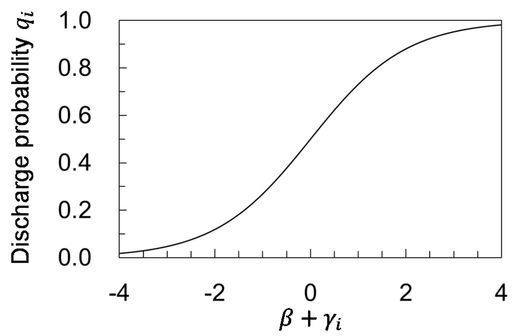
Examination of the constant discharge probability model demonstrates that it is unable to incorporate the dispersion in the actual discharge amount data into its mathematical expression. This arises from treating the discharge probability as a constant parameter. A resolution of this issue necessitates an improved model involving individual differences in the discharge probability among the vessels.

4.1. Formulation

In the variable discharge probability model, the discharge probability $q_i$ is regarded as a variable that depends on $i$, the index number of vessels. It is assumed to have a relation to parameters $\beta$ and ${\gamma }_i$ as follows:

$$\log \frac{q_i}{1-q_i}=\beta +{\gamma }_i, i=1,\cdots , N$$

(2)

which is generally referred to as the logit model, and the righthand side is referred to as linear predictor [11]. $\beta$ is the parameter of discharge amount that all the vessels have in common, hereafter referred to as the common parameter; ${\gamma }_i \left(i=1,\cdots , N\right)$ is the parameter of discharge amount that varies for each vessel, hereafter referred to as the individual parameter. Rearranging Equation (2) gives the discharge probability $q_i$ as

$$q_i=\frac{1}{1+\exp \left\{-\left(\beta +{\gamma }_i\right)\right\}}$$

(3)

which gives $q_i$ monotonically increasing against $\beta +{\gamma }_i$ (Figure 3).

The parameters $q_i$, $\beta$, and ${\gamma }_i$ vary stochastically. This aspect is in contrast to the constant discharge probability model. Distributions of $\beta$ and ${\gamma }_i$ are described in terms of other parameters, which are referred to as hyperparameters in the framework of the hierarchical Bayesian model [12].

The prior probability of the parameter $\beta$ is assumed to follow the normal distribution, expressed as

$$p\left(\beta |{\sigma }_{\beta }\right)=\frac{1}{\sqrt{2\pi {\sigma }_{\beta }}}\exp \left(-\frac{{\beta }^2}{2{\sigma }_{\beta }{}^2}\right),$$

(4)

where ${\sigma }_{\beta }$ is a hyperparameter that quantifies the variance of the parameter $\beta$ and is assumed to be a constant of 10.0, which is an uninformative prior.

The prior probability of the parameter ${\gamma }_i$ follows the normal distribution as

$$p\left({\gamma }_i|\sigma \right)=\frac{1}{\sqrt{2\pi \sigma }}\exp \left(-\frac{{\gamma }_i{}^2}{2{\sigma }^2}\right), i=1, \cdots , N$$

(5)

where $\sigma$ is also a hyperparameter that characterizes the Gaussian curve expressed by Equation (5) and is assumed to follow a uniform distribution.

Multiplying Equation (4) by Equation (5) yields the final form of the prior distribution as

$$\begin{array}{c}p\left({\gamma }_1,\cdots ,{\gamma }_N|\sigma \right) p\left(\beta |{\sigma }_{\beta }\right)={\displaystyle \prod _{i=1}^N}p\left({\gamma }_i|\sigma \right) p\left(\beta |{\sigma }_{\beta }\right) \hfill \\ \hfill =\frac{1}{\sqrt{2\pi }\sigma }{e}^{-\frac{{\gamma }_1{}^2}{2{\sigma }^2}}\ast \cdots \ast \frac{1}{\sqrt{2\pi }\sigma }{e}^{-\frac{{\gamma }_N{}^2}{2{\sigma }^2}}\ast \frac{1}{\sqrt{2\pi }{\sigma }_{\beta }}{e}^{-\frac{{\beta }^2}{2{\sigma }_{\beta }{}^2}}\end{array}$$

(6)

The formulation of the prior distribution is followed by the formulation of a likelihood which conveys the information from observations into a model. In a manner similar to the preceding section, the probability of bilge water discharge from the i-th vessel ($i=1, \cdots , N$) follows the binomial distribution as follows:

$$p\left(k_1,\cdots ,k_N|\beta ,\sigma ,r_1,\cdots ,r_N\right)={\displaystyle \prod }_{i=1}^{N}p\left(k_i|\beta ,\sigma ,r_i\right)={\displaystyle \prod }_{i=1}^N\left(\begin{array}{c}{N}_{\mathrm{d}}\\ k_i\end{array}\right)q_i{}^{k_i}{\left(1-q_i\right)}^{N_{\mathrm{d}}-k_i}$$

(7)

where $k_i$ denotes the discrete value of discharge amount from the i-th ship.

Using Equations (6) and (7) and according to Bayes’ theorem, the posterior probability distribution is written as,

$$p\left(\beta ,\sigma ,r_1,\cdots ,r_N|k_1,\cdots ,k_N\right)=\frac{p\left(k_1,\cdots ,k_N|\beta ,\sigma ,r_1,\cdots ,r_N\right) p\left({\gamma }_1,\cdots ,{\gamma }_N|\sigma \right) p\left(\beta |{\sigma }_{\beta }\right)}{p\left(k_1,\cdots ,k_N\right)}$$

(8)

where $p\left(k_1,\cdots ,k_N\right)$ denotes the probability that the data $k_1,\cdots ,k_N$ occur, which is independent on the parameters $\beta ,\sigma ,r_1,\cdots \cdots ,r_N$, and is thus treated as a constant.

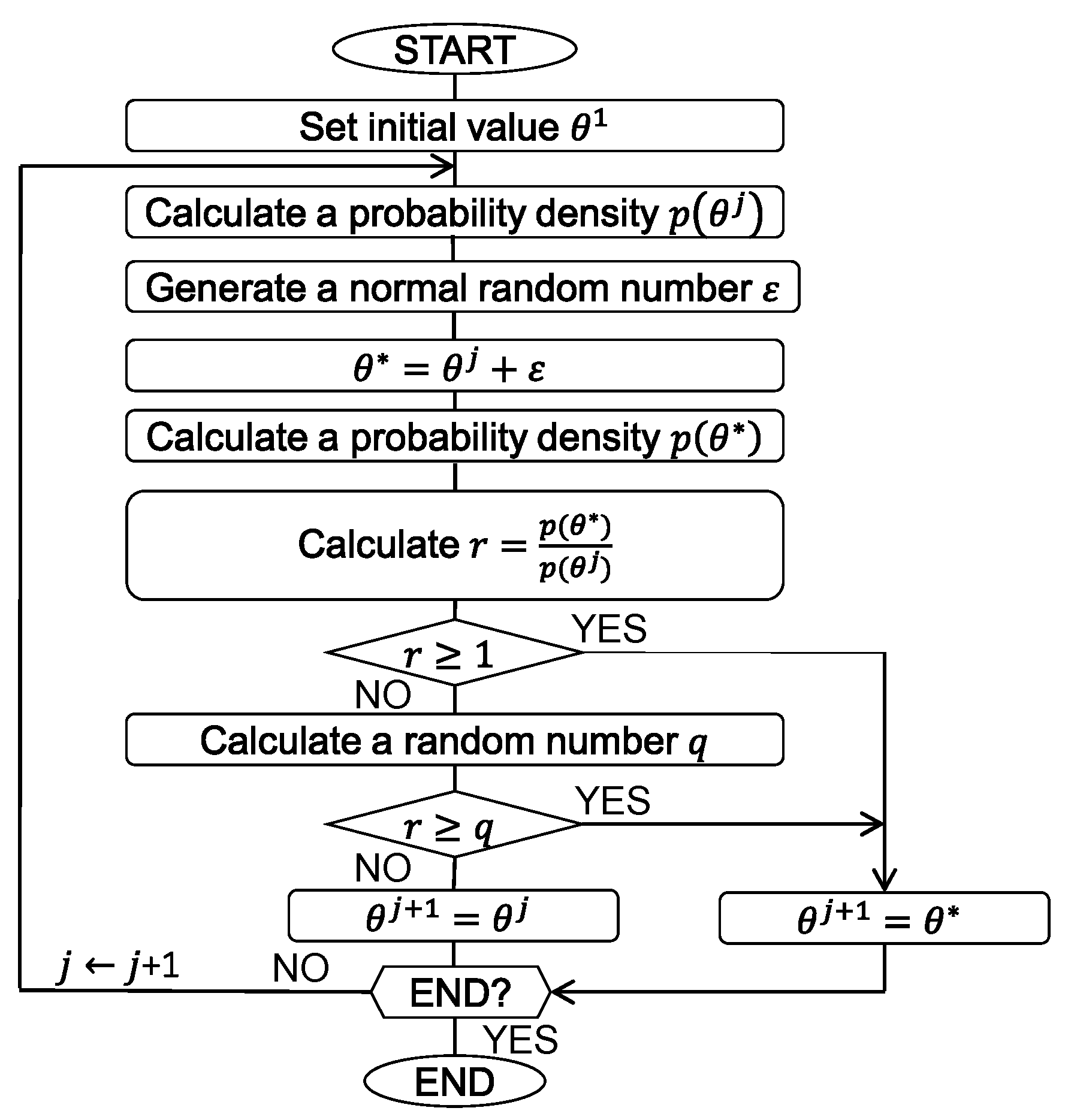
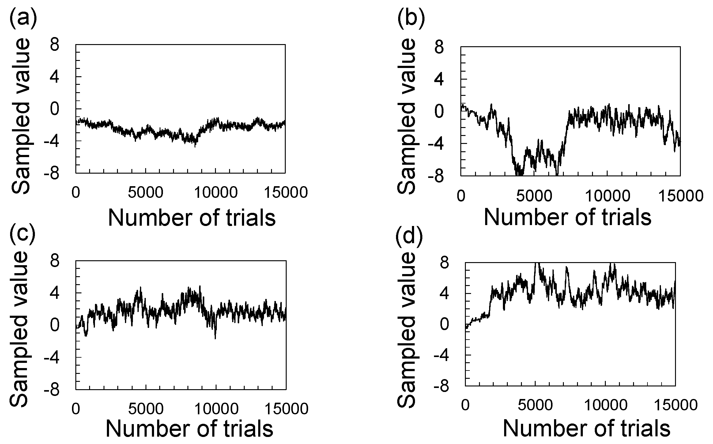
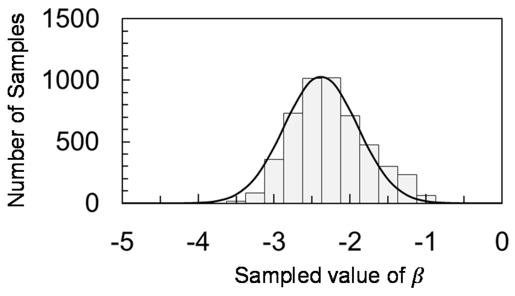
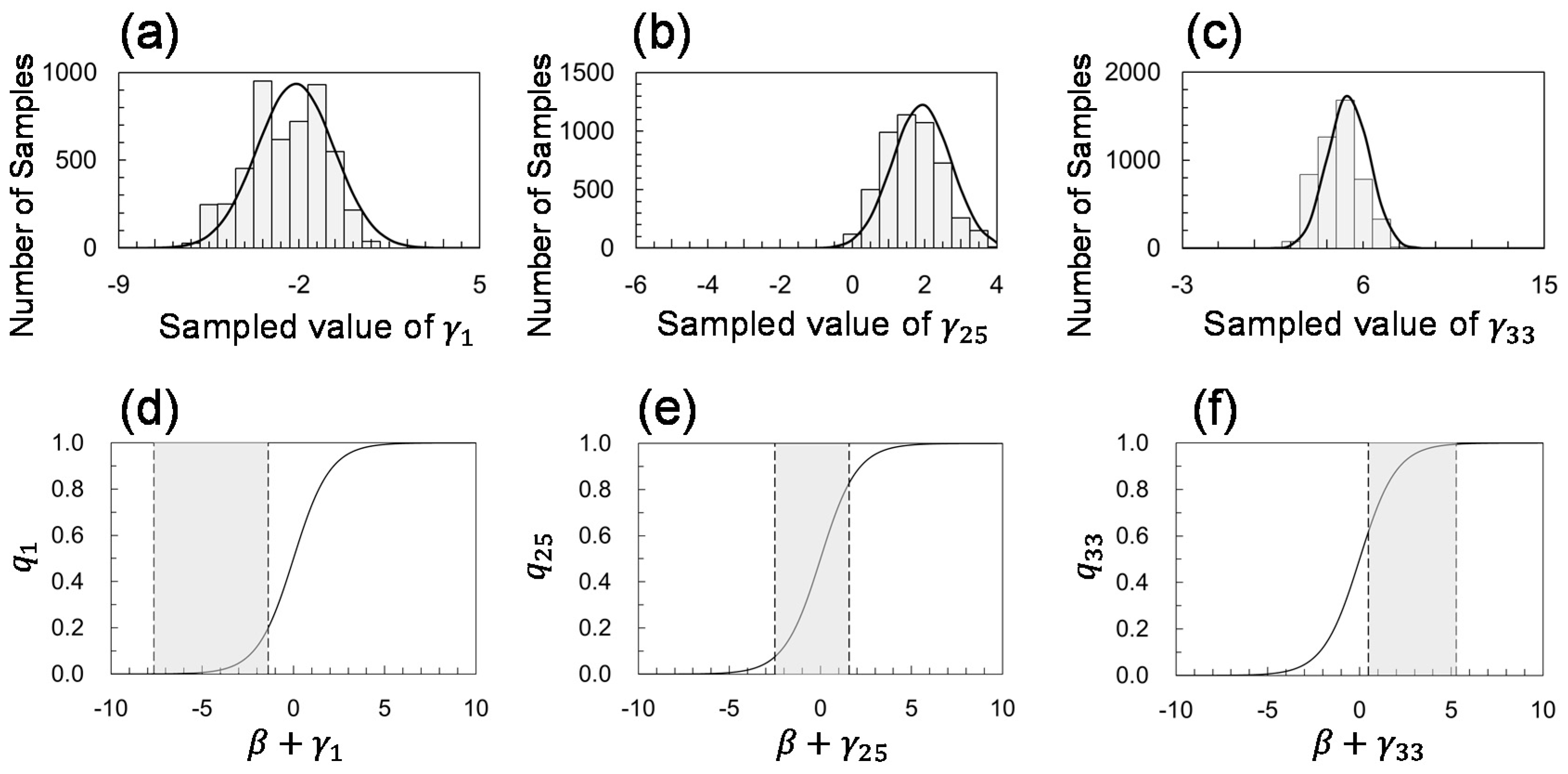
4.2. Numerical Method for Parameter Specification

This study applied the Metropolis-Hastings algorithm, one of the Markov Chain Monte Carlo (MCMC) methods [13], to the calculation of the posterior probability. In the MCMC method, numerous samples of a stochastic variable are randomly taken according to a probability density, and as the samples increase, the discrete set of samples gradually better approximates the continuous distribution of the probability.

Let $\theta$ be a parameter to which we hope to make inference. The Metropolis-Hastings algorithm generates random samples by consecutively proposing a new value${\theta }^{*}$ (Figure 4). If this proposed value is accepted according to a criterion mentioned below, it is set to be the next value ${\theta }^{j+1}$, where $j$ is a sampling sequence. If the proposed value is rejected, the previous value is retained, i.e., ${\theta }^{j+1}={\theta }^j$.

The criterion of whether a proposition is accepted or rejected computes a probability density $p\left( {\theta }^{*}\right)$, which is in proportion to the posterior probability and, accordingly, also in proportion to the likelihood. Then, the acceptance probability, defined as $r\equiv p\left( {\theta }^{*}\right)/p\left( {\theta }^j\right)$, is computed. With a probability of $\min \left(1, r\right)$, the proposition is accepted. Otherwise, it is rejected with a probability of $1-\min \left(1, r\right)$. When the number of samples grows enough, most of the disturbances involved in the initial guess of the parameters are removed and, consequently, a distribution of the samples with a density proportional to the posterior probability is determined.

4.3. Results and Discussion of Variable Discharge Probability Model

Trace plots of some parameters (Figure 5) generated by MCMC sampling had increasing and decreasing trends, which resulted from the disturbances due to the initial guess of the parameters. To prevent the trends from affecting analyses of the posterior distribution, the first 3000 samples were discarded as burn-in, the remaining samples were used for the analyses.

To see the relationship of numbers of vessels with the bilge water discharge amount, products of $q_i$ and $N_d$ (expected discharge amounts of each vessel) were computed for $i=1, \cdots , N$. Then, numbers of the vessels were counted for each discrete discharge amount. The numbers obtained in this way were compared with the number of vessels based on the observation (Figure 6). The model was well consistent with the observation, and the variance calculated by the model was markedly improved compared to the variance obtained by the constant discharge probability model (Table 2).

The MCMC method generated the samples that approximate the posterior distributions of $\beta$ and ${\gamma }_i$. They were used to analyze the statistical properties of these parameters. Figure 7 and Figure 8 show examples of the histograms of those samples and of the posterior distributions constructed using the histograms. Averages and 90% confidence intervals of $\beta$ and ${\gamma }_i$ were calculated from the posterior distributions.

The distributions of $\beta$ and ${\gamma }_i$ determine the distributions of the discharge probability $q_i$(Figure 8). The differences in $q_i$ among the vessels arise from the individual parameter ${\gamma }_i$. Factors causing the discharge are discussed by examining ${\gamma }_i$. As expected, the computed individual parameter ${\gamma }_i$ was larger for a larger discharge amount (Figure 9). A closer examination of the relationship between ${\gamma }_i$ and the discharge amount provides insight into the effect of the IBTS. The averages of ${\gamma }_i$ were computed separately for the vessels with and without the IBTS (

Table 3. Mean of individual parameter $r_i$.

With IBTS	Without IBTS
−1.571	1.233

). The comparison of ${\gamma }_i$ for the vessels with and without the IBTS shows that the IBTS certainly reduced the bilge water discharge amount.

This was also demonstrated by analyzing the relationship of ${\gamma }_i$ to the year of construction (Figure 10). Relatively new vessels constructed in the 1990s and 2000s were equipped with the IBTS and exhibited low ${\gamma }_i$ values. Under the MARPOL 73/78, the oil content of discharged effluent must not exceed 15 ppm. Both this regulation and the IBTS installation unquestionably suppressed the amount of discharge.

Next, by examining ${\gamma }_i$ in terms of the types of vessel, the question of which type of vessel has an especially large amount of discharge can be answered. Figure 11 depicts the individual parameter ${\gamma }_i$ versus ship type. Whereas the vessels with the IBTS overall had smaller ${\gamma }_i$ values than the vessels without the IBTS, special attention should be paid to the fact that ${\gamma }_i$ of the vessels without the IBTS varied depending on the ship type. Container ships had a larger ${\gamma }_i$ than the other types. The values of ${\gamma }_i$ for two of the three container ships listed in Table 1 exceeded or approached the limit of the 90% confidence interval. To more clearly bring confirmation of the dependence of ${\gamma }_i$ on the ship type, the averages of ${\gamma }_i$ were computed for each ship type (

Table 4. Mean of individual parameter $r_i$ for various ship types. PCC and VLCC stand for pure car carrier and very large car carrier, respectively.

	With IBTS	Without IBTS
Bulk	−1.615	−0.060
Container	−1.794	2.919
PCC	−1.594	−0.259
Tanker	−1.029	1.200
VLCC	0.065	1.420
Unknown	−2.765	1.631

). The container ships and unknown ships had greater averages of ${\gamma }_i$ than the other ship types.

Those results indicate that the container-type ship is somehow linked with the discharge of larger amounts of bilge water, and can be regarded as a secondary factor, while the absence of the IBTS constitutes the primary factor. Plotting the individual parameter ${\gamma }_i$against ship size (gross tonnage (GT)) shows that the vessels of around 40000 GT had extremely large discharge amounts (Figure 12), which exceeded the 90% confidence interval.

It follows that the container-type ship and/or the vessel size of about 40000 GT were linked to a very large amount of bilge water discharge. It is unlikely, however, that ship size alone is related to the increase in the discharge. Technological problems might exist in the structural design of container ships without the IBTS, and/or there might be careless handling of the bilge water in those vessels.

The statistic model enables us to consider the uncertainties involved in the original data and, accordingly, to use results of the model to predict the bilge water discharge amount for a variety of vessels and propose an adequate strategy to improve ship designs toward smaller amounts of bilge water discharge.

5. Conclusions

For the purpose of identifying the major contributing factors of bilge water discharge from ships into the surrounding marine environment during normal operations, this study developed a statistical model that expresses the relationship of the amount of bilge water discharge with a few explanatory variables. This study collected as much data on bilge water as possible and used them to build the statistical model according to Bayesian statistics. Parameters included in the model were determined by applying the Metropolis-Hastings algorithm, one of the MCMC methods. The examination of the model results confirmed that the model well represents the expected values and variances of the probability distribution of the discharge amount. Interpretations of those parameters showed that the container-type ship is related to notably large amounts of bilge water discharge, while this large amount of discharge arises principally from the absence of the IBTS in the vessels.

References

1. Geyer, R.A. Marine Environmental Pollution, 1 Hydrocarbon; Elsevier: Amsterdam, The Netherlands, 1980; p. 591. [Google Scholar]
2. Gerhard, W.A.; Lundgreen, K.; Drillet, G.; Baumler, R.; Holbech, H.; Gunsch, C.K. Installation and use of ballast water treatment systems—Implications for compliance and enforcement. Ocean Coast. Manag. 2019, 181, 104907. [Google Scholar] [CrossRef]
3. National Research Council. Oil in the Sea III Inputs, Fates, and Effects; National Academy of Sciences: Washington, DC, USA, 2002; p. 265. [Google Scholar]
4. United States Environmental Protection Agency. Vessel General Permit; United States Environmental Protection Agency: Washington, DC, USA. Available online: https://www.epa.gov/npdes/vessels-vgp (accessed on 20 February 2020).
5. Billheimer, D. Compositional receptor modeling. Environmetrics 2001, 12, 451–467. [Google Scholar] [CrossRef]
6. Hayashi, T.I.; Kashiwagi, N. A Bayesian approach to probabilistic ecological risk assessment: Risk comparison of nine toxic substances in Tokyo surface waters. Environ. Sci. Pollut. Res. 2011, 18, 365–375. [Google Scholar] [CrossRef] [PubMed]
7. International Maritime Organization. Work Programme of the Committee and Subsidiary Bodies, the Concept of the Integrated Bilge Water Treatment System (IBTS) and the Bilge Volume Generated in IBTS Machinery Space. Marine Environment Protection Committee (MPEC) 51/6, Agenda item 20; International Maritime Organization: London, UK, 2004. [Google Scholar]
8. International Maritime Organization. Measures to Promote Integrated Bilge Water Treatment System, Proposal for Promotion of Integrated Bilge Water Treatment Systems (IBTS). Sub-Committee on Ship Design and Equipment (DE) 54/17, Agenda Item 17; International Maritime Organization: London, UK, 2010. [Google Scholar]
9. Ueda, K.; Yamanouchi, H.; Hatori, K.; Yamane, K.; Yoshida, K.; Aya, T.; Sakane, Y.; Iijima, N. Treatment measures of engine room bilge. Proc. Natl. Marit. Res. Inst. Annu. Res. Present. 2004, 4, 261–264. [Google Scholar]
10. Organization for Economic Co-operation and Development (OECD). Cost Savings Stemming from Non-Compliance with International Environmental Regulations in the Maritime Sector, DSTI/DOT/MTC (2002)8/FINAL; Organization for Economic Co-operation and Development (OECD): Paris, France, 2003. [Google Scholar]
11. Dobson, A.J.; Barnett, A.G. An Introduction to Generalized Linear Models, 3rd ed.; CRC Press: Boca Raton, FL, USA, 2008; p. 307. [Google Scholar]
12. Gelman, A.; Carlin, J.B.; Stern, H.S.; Dunson, D.B.; Vehtari, A.; Rubin, D.B. Bayesian Data Analysis, 3rd ed.; CRC Press: Boca Raton, FL, USA, 2013; p. 661. [Google Scholar]
13. Gilks, W.R.; Richardson, S.; Spiegelhalter, D.J. Markov Chain Monte Carlo in Practice; Chapman & Hall/CRC: London, UK, 1996; p. 486. [Google Scholar]
Figure 1. Log-likelihood versus discharge probability.
Jmse 08 00320 g001
Figure 2. Number of vessels versus amount of discharge. Solid line is from the constant discharge probability model, and closed circles are from observation.
Jmse 08 00320 g002
Figure 3. Growth curve representing relationship between discharge probability and parameters used in variable discharge probability model.
Jmse 08 00320 g003
Figure 4. Flowchart of Metropolis–Hastings algorithm.
Jmse 08 00320 g004
Figure 5. Trace plots of sampled values of parameters versus number of trials. (a) Common parameter β , and individual parameters: (b) γ 1 , (c) γ 25 , and (d) γ 33 .
Jmse 08 00320 g005
Figure 6. Number of vessels versus amount of discharge. Solid line is from the variable discharge probability model, and closed circles are from observation.
Jmse 08 00320 g006
Figure 7. Histogram for sampled values of common parameter β generated by the Markov Chain Monte Carlo (MCMC) method. Solid line is normal distribution that approximately fits the histogram.
Jmse 08 00320 g007
Figure 8. Histograms for sampled values of individual parameters: (a) r 1 , (b) r 25 , and (c) r 33 . Solid lines are normal distributions that approximately fit the histograms. Discharge probabilities q i versus (d) β + r 1 , (e) β + r 25 , and (f) β + r 33 . In (df), 90% confidence intervals of β + r i are gray-hatched. Ranges in vertical axis corresponding to hatched regions are intervals of q i .
Jmse 08 00320 g008
Figure 9. Relationship between bilge water amount and individual parameters. Opened and closed circles are plots for vessels with IBTS and without IBTS, respectively. Solid line is mean of individual parameters, and dashed lines are upper and lower limits of 90% confidence interval.
Jmse 08 00320 g009
Figure 10. Relationship between construction year and individual parameters. Opened and closed circles are plots for vessels with IBTS and without IBTS, respectively. Solid line is mean of individual parameters, and dashed lines are upper and lower limits of 90% confidence interval.
Jmse 08 00320 g010
Figure 11. Relationship between ship type and individual parameters for vessels (a) with IBTS and (b) without IBTS. PCC and VLCC stand for pure car carrier and very large car carrier, respectively.
Jmse 08 00320 g011
Figure 12. Relationship between ship size and individual parameters. Opened and closed circles are plots for vessels with IBTS and without IBTS, respectively. Cross symbols are plots for vessels for which information on the install of IBTS was unavailable. Solid line is mean of individual parameters, and dashed lines are upper and lower limits of 90% confidence interval.
Jmse 08 00320 g012