Article

A New Method for Extracting Laver Culture Carriers Based on Inaccurate Supervised Classification with FCN-CRF

College of Geomatics, Shandong University of Science and Technology, Qingdao 266590, China
*
Author to whom correspondence should be addressed.
J. Mar. Sci. Eng. 2020, 8(4), 274; https://doi.org/10.3390/jmse8040274
Submission received: 18 February 2020 / Revised: 7 April 2020 / Accepted: 9 April 2020 / Published: 11 April 2020

Abstract

:
Timely monitoring of marine aquaculture has considerable significance for marine ecological protection and maritime safety and security. Considering that supervised learning needs to rely on a large number of training samples and the characteristics of intensive and regular distribution of the laver aquaculture zone, in this paper, an inaccurate supervised classification model based on fully convolutional neural network and conditional random filed (FCN-CRF) is designed for the study of a laver aquaculture zone in Lianyungang, Jiangsu Province. The proposed model can extract the aquaculture zone and calculate the area and quantity of laver aquaculture net simultaneously. The FCN is used to extract the laver aquaculture zone by roughly making the training label. Then, the CRF is used to extract the isolated laver aquaculture net with high precision. The results show that the k a p p a coefficient of the proposed model is 0.984, the F 1 is 0.99, and the recognition effect is outstanding. For label production, the fault tolerance rate is high and does not affect the final classification accuracy, thereby saving more label production time. The findings provide a data basis for future aquaculture yield estimation and offshore resource planning as well as technical support for marine ecological supervision and marine traffic management.

1. Introduction

Laver aquaculture is an important part of the marine fishery economy and occupies an absolutely dominant position in aquaculture. However, with the development of the economy, the rapid growth of laver aquaculture zones has also brought about marine environmental problems, such as green tides [1]. On the other hand, the large-scale reproduction of enteromorpha will cover the aquaculture boxes and suspended nets, thereby hiding the mariculture zone, which may affect marine traffic and port transportation. Therefore, monitoring the growth status and coverage of laver and other marine products in a timely manner is highly important [2].
Routine identification and management methods of the laver aquaculture zone mainly include the use of statistics on the sea area application and confirmation of the registration records of the farmers. This method can ensure accuracy of sea area usage statistics but involves a large workload and a long cycle, and thus, it should not be used as the mainstream method for the identification and monitoring of aquaculture areas [3]. Satellite remote sensing technology has become an important means of surface monitoring because it is not restricted by time and space and has a wide coverage area [4]. Various methods have been formulated based on remote sensing technology, including the visual interpretation method, traditional classification method based on spectral statistics, morphological classification method, and object-oriented method. The visual interpretation method based on expert experience [5,6] can reflect the aquaculture area and location more realistically. However, although this method can meet the requirements of a classified survey, it involves a large amount of work, takes a long time, and has high requirements for interpreters and poor universality. Some researchers in Reference [7] completed the automatic extraction of offshore aquaculture zones based on spectral information but with low precision and data redundancy. The authors in Reference [8] used edge detection and multi-scale feature fusion to extract the shape and texture information of the aquaculture zone and then extract the aquaculture zone. This method can realize the automatic extraction of different types of aquaculture zones with high precision but has higher requirements on data sources. Pixel-based experimental analysis is difficult to use in solving the phenomenon of salt and pepper noise due to large internal error between high spatial resolution. The authors in Reference [9] overcame the salt and pepper noise by using the object-oriented extraction method. However, classification accuracy for this method depends on the segmentation scale, the accurate acquisition of the sample, and the construction of the feature space. These elements need to be reconstructed as the image is updated, making it difficult to repeat.
Recently, deep learning has achieved remarkable achievements in object recognition, image classification, and other fields of machine vision. Deep learning models rely on multiple neural network layers to learn representations of data with multiple levels of abstraction. These methods fit the model through forward calculation and the backpropagation algorithm to achieve the optimal state of the model, and finally realize the purpose of data recognition, classification, and prediction [10,11]. Networks such as RNN (recurrent neural network) and its variants, LSTM (long short-term memory), have memory function, which can keep the output of the neuron from the previous moment to the next moment [12,13], so they are more suitable for processing time series data, but they are slightly inferior to image classification problems. The authors in Reference [14] used the original fully connected neural network to identify different classes of thumbnails. The method is easy to implement, but it has a poor processing effect for complex experiments, such as more parameters and high dimensional data. Targeting the disadvantages of fully connected neural networks, the authors in References [15,16] proposed a convolutional neural network, which has the advantages of weight sharing, so it can greatly reduce the number of training parameters and improve training performance. Then, some researchers proposed AlexNet to classify the 1.2 million high-resolution images in the ImageNet LSVRC-2010 contest into the 1000 different classes. This method further improves the classification accuracy of convolutional neural networks [17]. However, the above networks do not consider the semantic information of the images, and cannot accurately classify the internal categories of the images. The aquaculture net contains a large amount of seawater information, which is actually a kind of noise, which will seriously affect the task of extracting and identifying the aquaculture net. The emergence of semantic segmentation methods has fully solved this problem, such as FCN (fully convolutional neural networks) [18,19,20,21], U-Net [22], Segnet [23], Deeplab series [24,25], and other semantic segmentation algorithms, which learn in end-to-end form, provide pixel semantic information to complete the pixel-level classification of images, and take into account the spectral, spatial, and contextual information, and have high classification accuracy. Among them, the FCN network is the forerunner of semantic segmentation, whose main characteristics are encoding-decoding structure and skip connection. Most semantic segmentation networks are improved based on the FCN structure.
The above methods belong to the category of supervised learning. They rely on a large number of training samples and can only extract the aquaculture zone and cannot accurately count the number of aquaculture carriers in the aquaculture zone. In addition, the repeated down-sampling of the image by FCN will result in the loss of a large amount of edge information and make the pixels at the edge of the object smoother. Moreover, convolution only extracts local receptive fields. Although repeated extraction can eventually cover the entire image, the correlation between a pixel and all other pixels in the whole image cannot be extracted, even at the last convolutional layer. Conditional random filed (CRF) is a learning model that generates pixel classification results by calculating the position and color relationships of each pixel and all other pixels in the image, thereby providing a new idea for accurately extracting culture carriers in the aquaculture zone. Based on the characteristics of dense and regular distribution of seawater and nets in the laver aquaculture zone, an inaccurate supervised classification method based on FCN and CRF is proposed. The Lianyungang laver aquaculture area in Jiangsu Province is taken as the research area to design a classification model that can extract the aquaculture zone and count the area and quantity of the laver aquaculture net simultaneously.

2. Materials and Methods

2.1. Materials

This study selected the offshore area of Lianyungang City, Jiangsu Province, as the study area to verify the accuracy and application performance of the model. The study area is distributed between 33°59′–35°07′ north latitude and 118°24′–119°48′ east longitude and located in the eastern coastal area of China, with the Yellow Sea adjacent to the east. It belongs to the temperate monsoon climate, cold and dry in winter, hot and rainy in summer. Due to its geographical advantages, it is less affected by waves, typhoons, and sea fog. Laver aquaculture zones are spread all over the sea area of Lianyungang, and the industry of laver aquaculture is the main economic component of marine aquaculture in Jiangsu Province. Therefore, it is more representative to select this research area for the extraction of laver culture carriers. An UAV (Unmanned Aerial Vehicle) image with a resolution of 0.1 m is used in this paper, which has 75,540 × 75,399 pixels. The image was obtained by aerial photography of a fixed-wing aircraft carrying a SonyA7R2 with 42 megapixels. It acquired 2216 images through three voyages 500 m above the ground. These images are stitched into the entire experimental image, as shown in Figure 1.

2.2. Principle

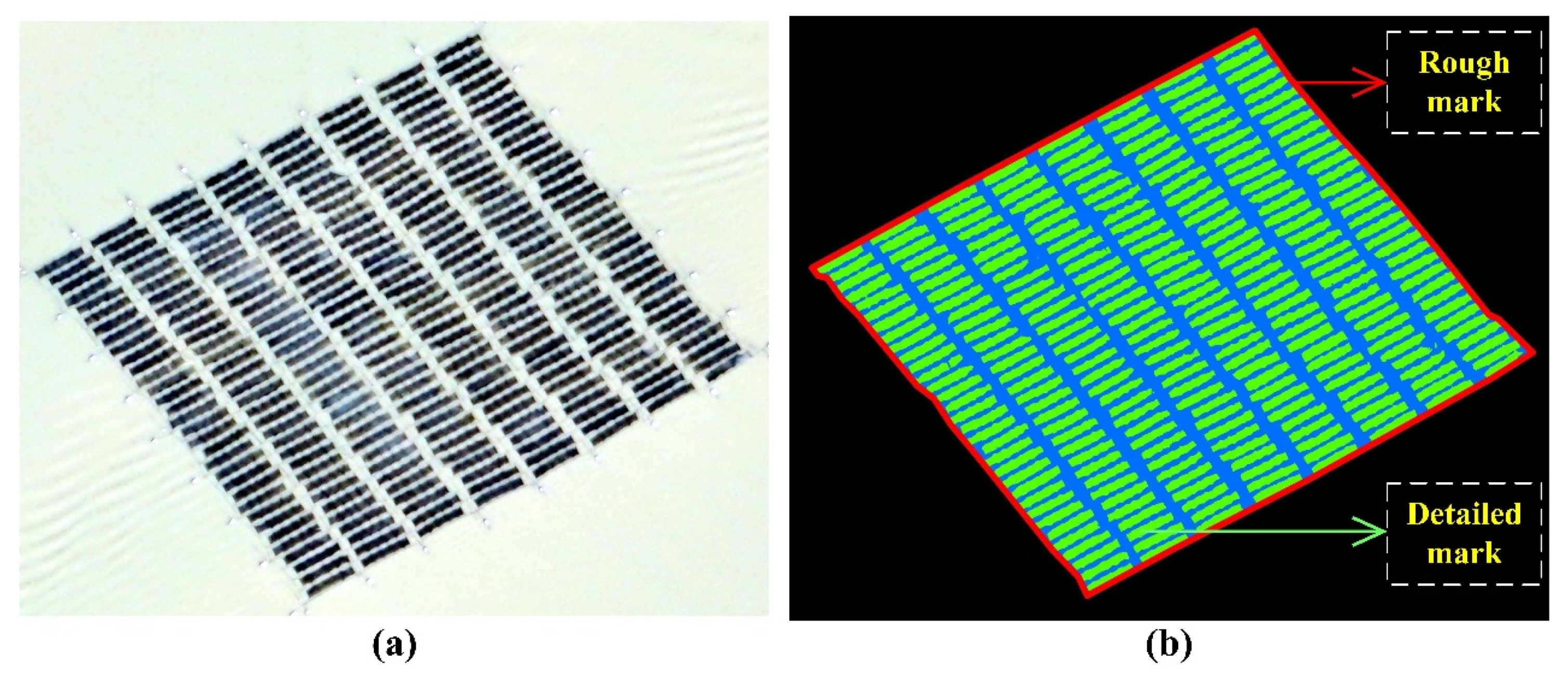
Inaccurate supervised classification involves marking the labels roughly and extracting the ground objects finely. In the culture zone, the aquaculture nets and seawater are staggered and arranged densely, making it cumbersome and time-consuming to mark labels for isolated single aquaculture nets. Therefore, rough labeling and fine classification are carried out in this paper to establish an inaccurate supervised classification model. The example is shown in Figure 2.
The rough mark means that the label is an aquaculture area that includes laver aquaculture nets and part of the seawater. Detailed mark means that the label only includes laver aquaculture nets.
The classification model is divided into two parts: FCN and CRF. FCN is used to extract the aquaculture zone and CRF is used to extract the border of the laver aquaculture net accurately and obtain the distribution of the laver aquaculture net to count the quantity and area of the nets.

2.2.1. FCN

Compared with the traditional convolutional neural network, FCN differs mainly from the convolutional layer instead of the fully connected layer, which can accept the input of images of any size and realize the pixel-level semantic segmentation through convolution and deconvolution structures [18].
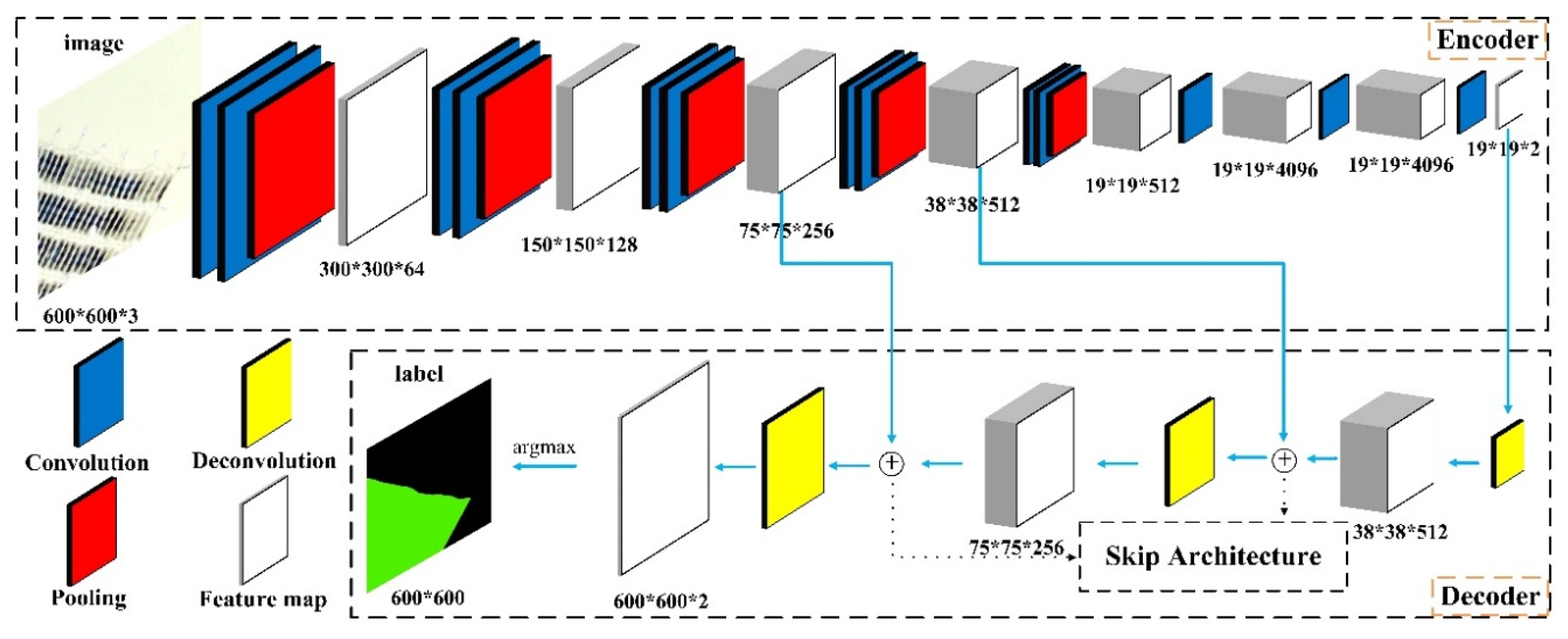
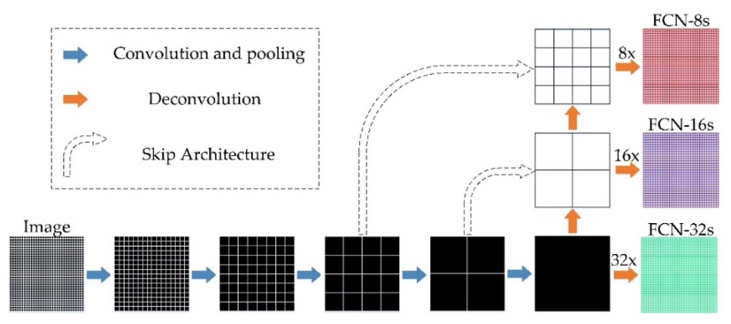
The FCN model is composed mainly of two parts: coding structure and decoding structure. The convolution layer in the coding structure extracts the image features in the window through the local receptive field each operation and the pooling layer performs mainly high-level extraction on the convolution features. The convolution layer and the pooling layer are matched alternately to complete the extraction of high-level features of the image. If the high-level features acquired by the coding structure are decoded directly to obtain the corresponding semantic information, the boundary information will be lost and the classification result will be rough. Therefore, the decoding process adds a skip architecture, which decodes the high-level features and combines the low-level features in the coding structure to optimize the output, and more refined semantic segmentation results are obtained. The network architecture is shown in Figure 3.
The upper part of Figure 3 is the coding structure of the FCN model, which is mainly used to extract high-level features step-by-step. The lower part is the decoding structure, which uses the skip architecture (Skip Architecture in Figure 3) to perform label prediction. It performs up-sampling through the high-level features extracted by the coding structure and combines the low-level features in front of the coding structure to obtain the prediction label of the image. The argmax function returns a higher probability class based on the network output class probability to generate a prediction result.
There are many adjustable parameters in the network model, such as learning rate, max-iteration, and batch-size. Among them, the learning rate is a hyperparameter that guides the network to adjust the network weight through the gradient of the loss function. The lower the learning rate, the slower the change of the loss function, but it is easy to reach a local minimum. The max-iteration refers to the number of times that the network performs self-fitting and self-optimization based on the training data. It is better to stop iteration after the loss has converged. The batch-size means the amount of data fed to the neural network in each batch, which can be adjusted according to the memory size.

2.2.2. CRF

CRF is a discriminative probability undirected graph learning model [26] with significant performance [27,28]. A rough segmentation may be generated in the details because of the independent label given to each pixel during the training of the FCN model. Therefore, the CRF is used in the network model to optimize the network results [29,30,31]. The input of the CRF contains the original image and the classification result of the FCN and aims to highlight the boundary information by minimizing the energy function of all pixel classification results information, position information, and channel information of the image. In the image, each pixel point I has pixel value X i and label value Y i ( Y i belongs to tag set L = { L 1 ,   L 2 ,   L 3 ...   L k }), taking each pixel as a node and the relationship between pixels as the edge to construct a conditional random airport. The conditional random field model conforms to the Gibbs distribution [32,33] shown in Equation (1):
P ( Y | X ) = 1 Z ( X ) exp ( E ( Y | X ) )
where Z ( X ) is the partition function and X is the fixed pixel point distribution. For convenience, the representation of X is omitted, and the Gibbs energy of y L is expressed as Equation(2):
E ( Y ) = i φ u ( y i ) + i < j φ p ( y i , y j )
where i φ u ( y i ) represents the unary potential function derived from the FCN classification result. The equation is as follows.
φ u ( y i ) = l n y i
where i < j φ p ( y i , y j ) represents the pairwise potential function, which describes the relationship between pixels. Similar pixels are assigned to the same label, otherwise, different labels are assigned. The equation is as follows:
φ p ( y i , y j ) = u ( y i , y j ) m 1 M ω ( m ) k G ( m ) ( f i , f j )
where u ( y i , y j ) is the label consistency function,   ω ( m ) is the Gaussian kernel corresponding weight, k G ( m ) is the Gaussian kernel, and f i ,   f j is the eigenvector of the pixels i and j .
k G ( m ) ( f i , f j ) = W ( 1 ) exp ( | p i p j | 2 2 θ 2 α | I i I j | 2 2 θ 2 β ) + W ( 2 ) exp ( | p i p j | 2 2 θ 2 γ )
The two-kernel potentials are defined in terms of the color vectors I i and I j and positions p i and p j . The first half represents the appearance kernel, nearby pixels with similar color are likely to be in the same class. The latter half represents the smoothness kernel, which is only related to the pixel position and can remove small isolated regions. These two kernels are controlled by the spatial standard deviation θ α and θ γ and the color standard deviation θ β .
Pairwise potential is mainly used to describe the relationship between all pixels in an image, which stimulates similar pixels to assign the same label. The criterion for judging similarity is related to the pixel value and the actual relative distance. Therefore, the CRF can compare each pixel in the image with all other pixels, and then obtain an accurate classification result under a global field of view based on the FCN result.

2.3. Methods

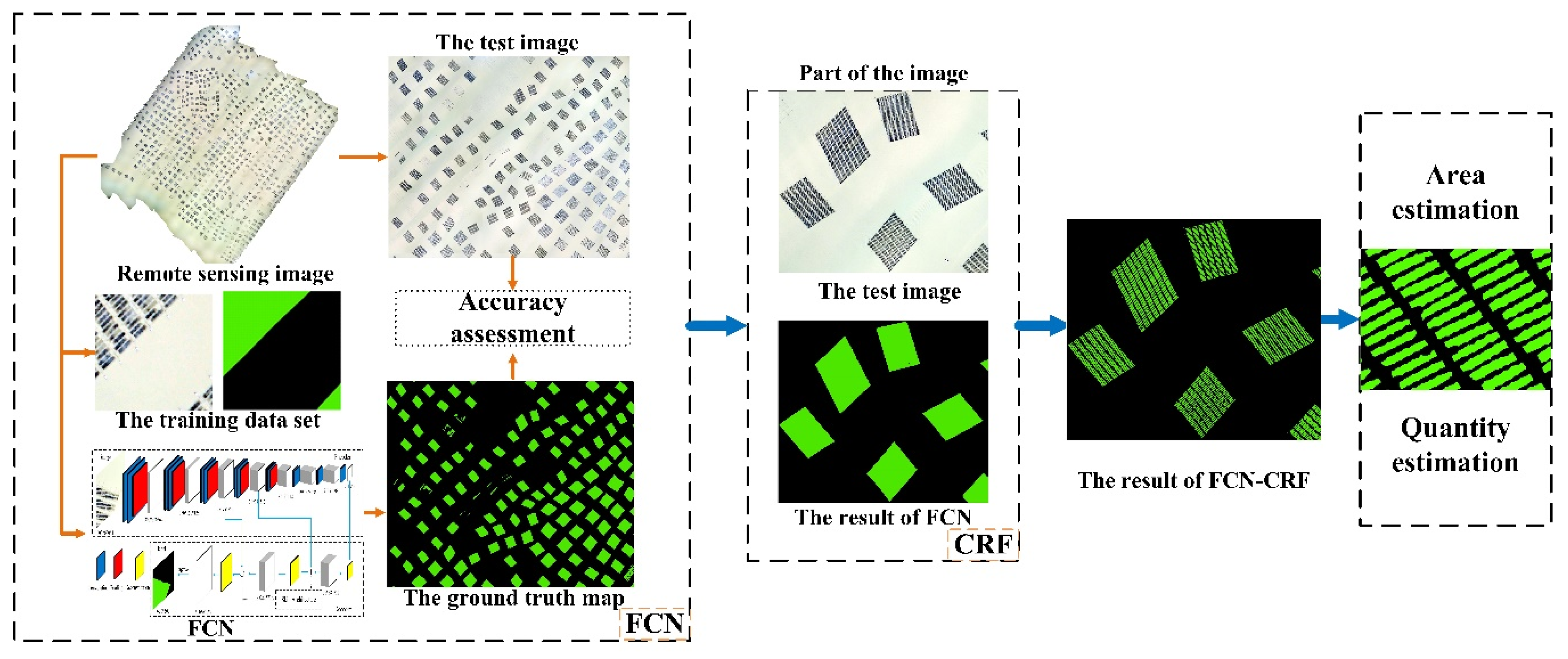
The methods in this paper are divided mainly into four parts: image preprocessing, FCN training and classification, accuracy evaluation, and CRF post-processing. The overall process is shown in Figure 4.

2.3.1. Image Preprocessing

To fully train the network, vectorizing the laver aquaculture zone and seawater in the study area image is necessary, that is, assign image label attributes artificially. To prevent the model from being unable to train because of insufficient GPU (Graphics Processing Unit) memory in the training process, the image and label should be clipped regularly into a slice image with a sheet size of 600 × 600 pixels. The clipped data should be divided into a training dataset and validation dataset. The training dataset is mainly used for optimization and adjustment of network model parameters. The validation dataset is used to verify the model accuracy and universality and adjust the network model hyperparameter. In addition, the test dataset is used for the final experimental classification to complete the semantic segmentation of the image.

2.3.2. FCN Training and Classification

After the experimental data is produced, through training, the model learns the data features and the loss function is used to give the fitting error while the back-propagation algorithm is used to adjust the network parameters until the model reaches the optimal state. The parameters, such as the max-iteration and learning rate, can be adjusted further according to the model validation accuracy and the final classification effect.

2.3.3. Accuracy Evaluation

FCN is compared with maximum likelihood classification (MLC), support vector machine (SVM), and neural network classification (NN) methods through the   k a p p a ,   p r e c i s i o n , r e c a l l , and F 1 . The equations are as follows:
k a p p a = ( P o P c ) / ( 1 P c )
p r e c i s i o n = T s / ( T s + F s )
r e c a l l = T s / ( T s + F o )
F 1 = 2 R p r e c i s i o n R r e c a l l / ( R p r e c i s i o n + R r e c a l l )
where T s is the correct aquaculture area, T o is the correct seawater range, F s is the wrong aquaculture area, and F o is the wrong seawater range. P o = ( T s + T o ) / ( T s + F s + T o + F o ) , P c = ( ( T s + F s ) ( T s + F o ) + ( F s + T o ) ( T o + F o ) ) / ( T s + F s + T o + F o ) 2 .

2.3.4. CRF Post-Processing and the Number and Area Calculation of Aquaculture Nets

The accurate strip distribution of the laver aquaculture net is obtained using CRF processing in the aquaculture zone exported by FCN. The net area of the aquaculture zone is obtained by the image resolution and the pixel statistics on the results. Finally, the raster-vector conversion is carried out on the results and the quantity of the net in the aquaculture zone is obtained statistically.

3. Results

3.1. Preparation for the Experiment

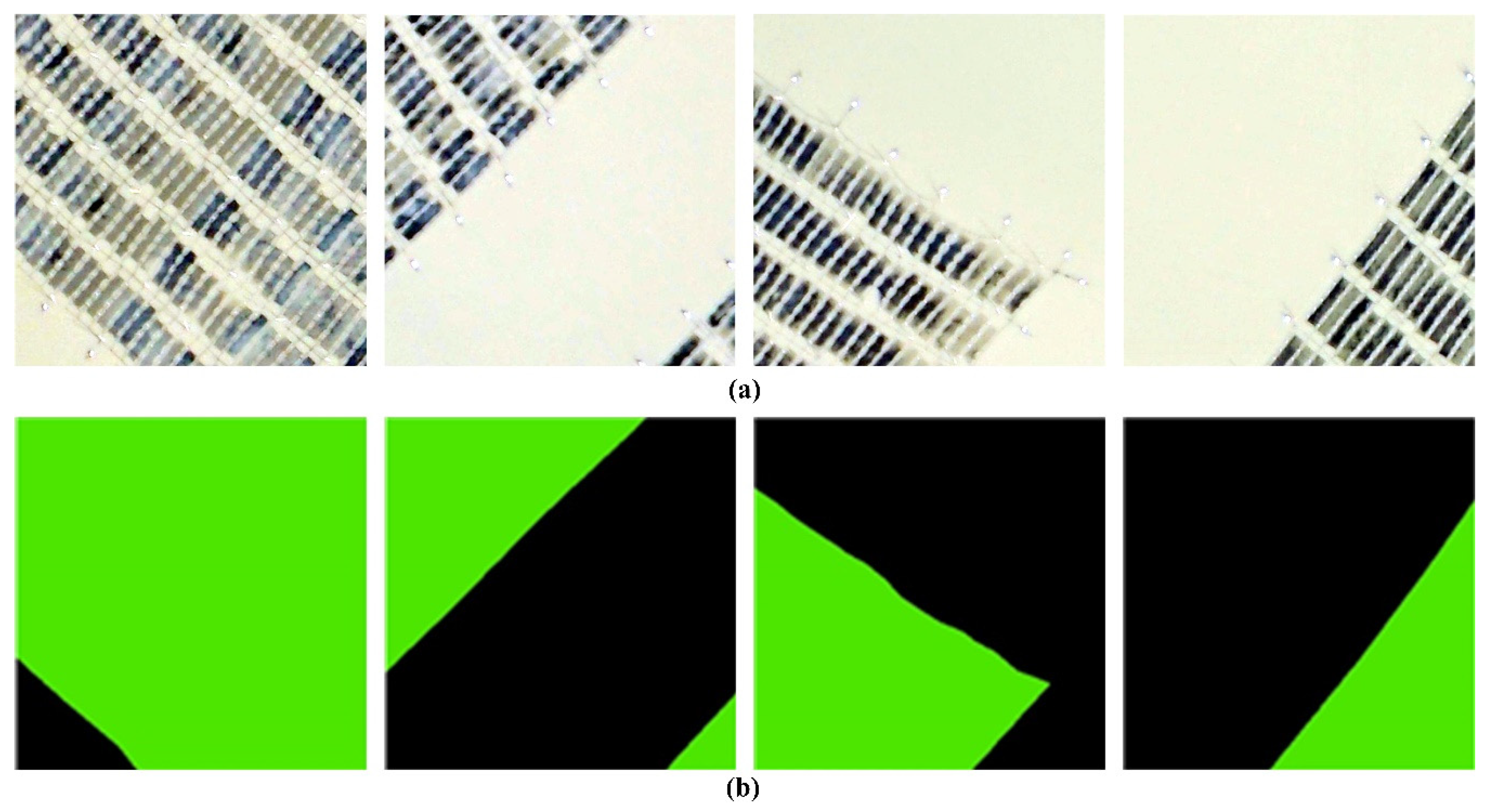
To facilitate the experiment, the images are labeled manually and divided into two categories: seawater and laver aquaculture zones. Seawater is assigned to attribute 1 and laver aquaculture zone is given attribute 0. In this paper, the number of training datasets is 1800 slice images and the validation dataset is 200. Some training data are shown in Figure 5.
Figure 5 shows that the image size is 600 × 600 pixels. The green part represents the laver aquaculture zone and the label attribute is 0, while the black part represents the sea area and the label attribute is 1. The labeling process does not distinguish between the seawater and the laver net inside the mariculture zone. The marked laver aquaculture zone contains a considerable amount of seawater information, which is an inaccurate label. The test image size is 19,988 × 23,949 pixels. Based on the Python language, Tensorflow and several function libraries such as gdal, numpy, and os, are used to build the experimental model. Tensorflow is a typical function library for deep learning. It has a complete data flow and processing mechanism, and encapsulates a large number of efficient algorithms and functions for neural network construction, which is very suitable for large-scale machine learning applications. The specific environment configuration is shown in Table 1.

3.2. Extracting Aquaculture Areas with FCN

As shown in Figure 6, FCN consists of FCN-8s, FCN-16s, and FCN-32s. Therefore, before using FCN to extract mariculture zones, a comparison and analysis of different parameter structures of FCN should be performed, and the best scheme will be selected to extract mariculture zones.
As shown in the figure above, the encoder in FCN structure reduces the image by 32 times through 5 times of pooling. The decoder of FCN-32s directly uses the result of the fifth pooling to generate the label corresponding to the input image through 32× up-sampling. The decoder of FCN-16s does not directly deconvolve the advanced features of the encoder, but uses 2× up-sampling, and combines the feature map of the fourth pooling layer of the encoder to obtain classification results by 16× up-sampling. On the basis of FCN-16s, FCN-8s continues to combine the feature map of the third pooling layer, and then obtains the semantic segmentation result consistent with the input image through 8× up-sampling. The results of FCN 8s, FCN 16s, and FCN 32s are shown in Table 2 and Figure 7.
By comparing the FCN of three different parameter structures, it can be seen that FCN-8s has the highest classification accuracy and the best output effect, and the other two methods are more likely to misclassify the fishing boat in the image into laver. FCN-16s only uses a skip structure to assist the decoder for up-sampling and cannot fully use the low-level features of the mariculture zones extracted by the encoder, so its output is not as good as FCN-8s. However, the way that FCN-32s directly obtains the output result by deconvolution is too rough, and the detailed information of FCN cannot be guaranteed, and the effect is the worst. The training of the FCN-8s, FCN-16s, and FCN-32s yields the cost function curve in Figure 8.
As show in Figure 8, each point of the curve in the figure is the average of the loss generated every 300 iterations. It can be seen that the FCN-8s has reached convergence at the 20,000th iteration, its convergence is the fastest and most stable. Therefore, this experimental model is based on FCN-8s (hereinafter referred to as FCN), and use the produced training set and validation set to train the network. The learning rate of the model is set as 0.0001 and the batch-size is 8. Adam optimizer and the cross-entropy loss function are adopted in the model, and many scholars use them to optimize the network to identify aquaculture zones and achieve remarkable results [34,35]. Adam is an algorithm for first-order gradient-based optimization of stochastic objective functions. It designs independent adaptive learning rates for different parameters and iteratively updates neural network weights based on training data. The Adam optimizer is simple, efficient, and requires less memory. The cross-entropy loss function can estimate the similarity between the prediction result and the sample label. The equation is as follows:
c = 1 n x [ y l a b l n y p r e + ( 1 y l a b ) l n ( 1 y p r e ) ]
where y l a b is the label (0 or 1), y p r e is the predicted value, x is the input value, and n is the number of x . The smaller the cross-entropy loss, the higher the prediction accuracy. When y p r e and y l a b are both 0 or 1, the value of the loss function is 0, indicating that the prediction is correct. This loss function can accelerate the convergence rate of the network. Finally, the test images are classified through 30,000 iterations of FCN. The classification results of FCN are compared with MLC, SVM, and NN, as shown in Figure 9.
Figure 9 shows that MLC, NN, and SVM can roughly identify the aquaculture area, but the MLC and SVM classification results have a lot of noise in the sea area. The large fishing boats and unclassified abandoned laver net piles are misclassified, which affects the classification accuracy. Although the NN classification results have improved the classification effect in the sea area, the aquaculture zone has a lot of noise, which destroys the integrity of the laver net and misclassifies the characteristic blurred area. However, the FCN can identify laver aquaculture zones fully without misclassification and the segmentation results are satisfactory, which is suitable for further extraction of subsequent classification models with inaccurate supervision.
The above method is evaluated quantitatively by k a p p a ,   p r e c i s i o n , r e c a l l , and F 1 , as shown in Table 3.
Table 3 shows that among the three classification methods of MLC, SVM, and NN, NN has the highest p r e c i s i o n at 96%, while the highest r e c a l l of SVM is 87%. FCN has a higher score in various accuracy indices than the other methods. The confusion matrix of the FCN classification results is shown in Table 4.
Table 4 shows that the label data of the mariculture zone have 103,255,518 pixels, and 102,061,026 pixels are classified correctly. The seawater label data have 375,437,094 pixels and the error classification is only 1,194,492 pixels. The recognition effect is positive. FCN has high recognition accuracy for the mariculture zone and is sufficient to complete the extraction of the mariculture zone with high precision. Using the pixel statistics of the results and the 0.1,m resolution, the test image area is 4,786,926.12 m2, in which the actual area of the mariculture zone is 1,032,555.18 m2 and the predicted area of the mariculture zone is 1,033,634.47 m2, with a statistical error of 0.1%.

3.3. Extracting Laver Aquaculture Nets with CRF

The laver aquaculture nets are obtained accurately by carrying out the CRF processing on the FCN classification result. The classification results of FCN are used to independently compute the unary potentials for each pixel, and set different adjustable parameters such as θ α , θ β , θ γ and epoch to generate the pairwise potentials of the conditional random field. In this paper, we designed four different experiments to extract nets and compare their effects. The experimental parameters are shown in Table 5.
Since θ γ had little effect on the result in the experiments, it is defined as 20 to play the best role. We cut out an image with 4183 × 4825 pixels from the experimental image as the data for this CRF experiment and used the above experiments with different parameters to extract the nets respectively. The extraction results of all schemes are shown in Figure 10.
From the comparison of CRF_1 and CRF_4 in the figure, it can be found that the fewer epochs of CRF, the more connections between the laver nets, and the worse the accuracy. When the epoch is gradually increased, the effect of the connection is obviously improved. When θ α and θ β are defined as 500 and 50, the net can be precisely extracted, and the internal structure of the aquaculture zone can be further refined. Because of the addition of the smoothness kernel into the pairwise potentials of the fully connected random field, the fishing boat in the purple box is not considered as laver and is correctly classified as the seawater part. That is, the CRF accurately classifies the seawater and laver strips in the undivided aquaculture zone during the labeling process. The shape and size of the classification results are similar to the images without damaging the accuracy of the FCN classification results. The inaccurate supervised classification process from the original image to the net of the aquaculture zone is realized. In order to study the results of CRF in detail, the classification results of the three red areas marked in the above figure are shown below in Figure 11.
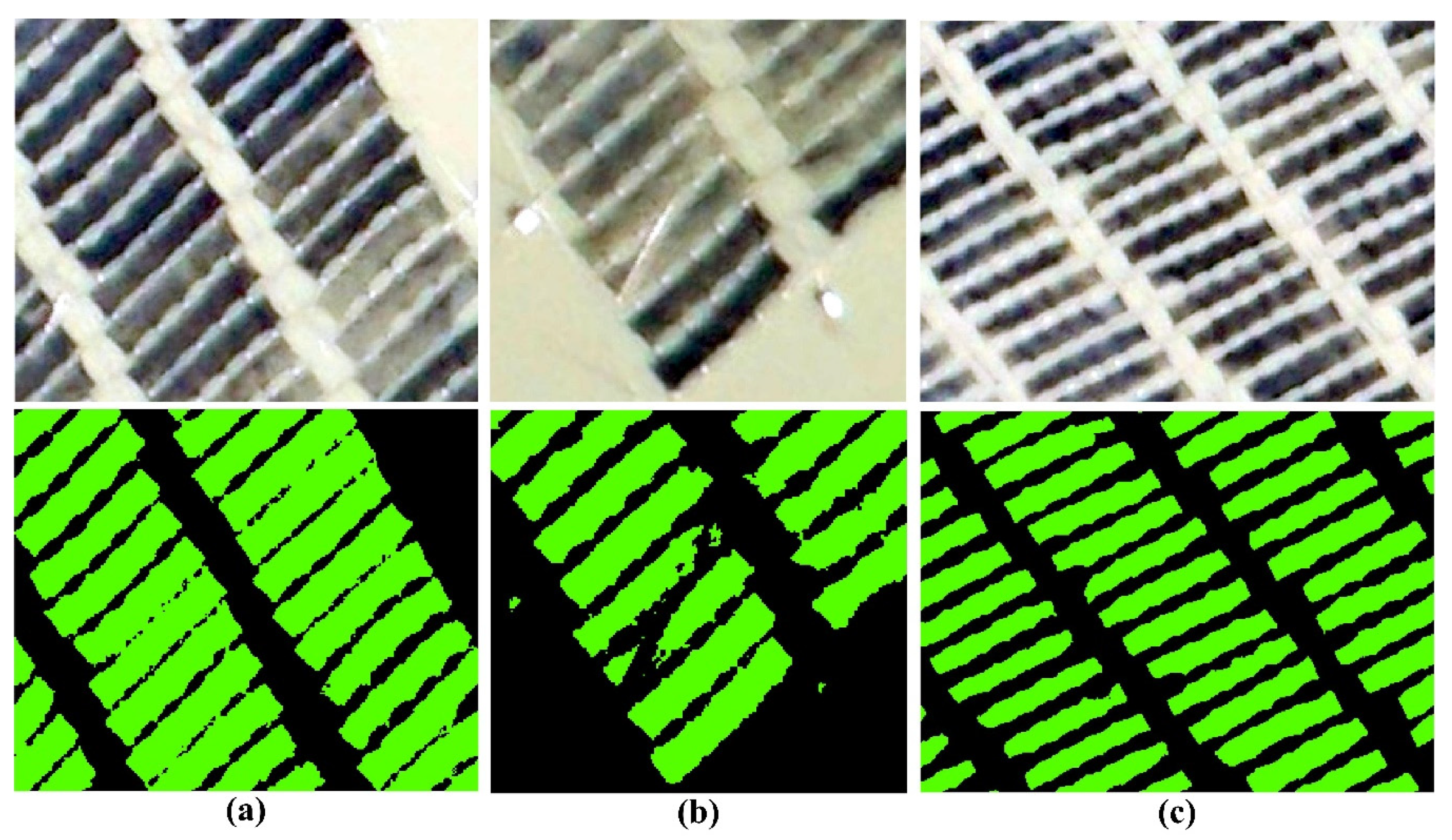
Figure 11a,b show that under-segmentation or over-segmentation can be observed in the fuzzy region mixed with other features and the floating objects on the sea will be misclassified. Meanwhile, for the clear and obvious feature in Figure 11c, the inaccurate supervised classification model based on CRF post-processing can extract the net individuals of the laver aquaculture zone accurately.
The fine area of the laver net strips in the aquaculture area can be obtained based on the results of the CRF treatment in Figure 10. Finally, the result of FCN-CRF treatment can be converted into a vector file through raster-vector conversion and the number of nets can be counted. The final experimental results are shown in Table 6.
Through experimental calculations, the total area of the image in Figure 10 is 201,829.75 m2, of which the area of the aquaculture zone is 45,301.04 m2, accounting for 22.45% of the total study area. The area of the net in the aquaculture zone is 25,220.45 m2, accounting for 55.67% of the aquaculture area and the seawater in the aquaculture area accounts for 44.33%, that is to say, the marked laver aquaculture zone contains more than 40% seawater, which is actually noise. The findings show that the proposed inaccurate classification model has a strong fault tolerance rate, and the total quantity of 1516 aquaculture screens is predicted. The quantity of screens (1501) in the aquaculture zone is obtained by visual interpretation. The results are very similar and have high reference values.

4. Discussion

In this paper, we designed an inaccurate supervised classification model for the extraction of laver aquaculture nets, which is mainly based on FCN and CRF. In the experiment, three different FCN structures of FCN-8s, FCN-16s, and FCN-32s were compared. Through the accuracy evaluation of the extraction results of the three methods with different parameters and the comparison of the effect display, it can be found that the FCN-8s with three skip architectures have the best results and had fully converged when the number of iterations reached 25,000. The FCN-32s that do not use skip architecture to combine the low-level features of the encoder and the FCN-16s that use only one skip architecture do not work well. They mistake the fishing boat for laver, lose the boundary information of the aquaculture zones, and generate more noise inside the classified aquaculture zones. Therefore, it is proven that the FCN-8s structure is the best, and it is more suitable for the extraction of aquaculture zones in areas with complex features than the other two structures. Then, this article used MLC, SVM, and NN to extract aquaculture zones. By comparing FCN with the above methods, we can see that the output of FCN has clearer boundaries and less noise, especially for abandoned aquaculture zones, FCN has better identification and there is almost no misclassification. After using FCN to extract aquaculture areas, we set up CRFs with different parameters for experiments and comparisons. It can be found that CRFs with higher epoch have higher recognition accuracy and are mainly affected by two parameters, θ α and θ β . After CRF processing, laver strips can be accurately extracted without damaging the output of FCN. We can count the number and area of nets based on the results of the CRF.
The previous studies extracted the aquaculture zones in the offshore area based on supervised classification, and did not divide the culture carriers inside the aquaculture zones. This only achieved a rough extraction of the aquaculture zones. If the internal carriers are segmented, more detailed labels are needed to train the network model. This method will inevitably increase the workload and preprocessing time of the experiment. The inaccurate supervised classification model we proposed can not only extract the laver aquaculture zones but also accurately obtain the area and quantity of culture carriers, which is beneficial to the management of marine resources. However, there are still many limitations in our research. For example, it is easy to mistakenly identify floating objects near the aquaculture zones as laver culture carriers, which will affect our final area statistics. On the other hand, the model in this paper contains more than 40% seawater information in the labeling process of the aquaculture zone, which has a high fault tolerance rate. This is mainly because the features in our study area are relatively single. Features include only aquaculture zones and seawater, which is quite advantageous for our model. We still have a lot of work to do to improve the universality of the model.

5. Conclusions

This paper designed an inaccurate supervised classification model in allusion to the characteristics of intensive and regular distribution of laver aquaculture zone and the problem that supervised learning requires a large number of samples. The proposed model can extract aquaculture zone and count the area and quantity of the laver aquaculture net simultaneously. The study area focused on the Lianyungang laver aquaculture zone of Jiangsu Province. The conclusions are as follows.
(1) The k a p p a coefficient of the classification results obtained by FCN-8s can reach 0.984 and F 1 was 0.99, which proves that the FCN network model can complete the classification of laver with high accuracy.
(2) Using CRF post-treatment, the individual laver aquaculture net can be divided accurately, and the overall effect was positive, which proves that the proposed model can extract the area and quantity of the laver cultivation net well and has higher reference value.
(3) The inaccurate supervised classification model can effectively identify the laver aquaculture zones and has a high fault tolerance rate, which can meet the requirements of the inaccurate supervised classification of the coarse label and fine classification. It saves considerable labeling time without affecting the final classification accuracy. The data provide a foundation for future laver farming estimation and offshore resource planning and technical support for marine ecological regulation and maritime traffic management.
Based on the analysis of the experimental conclusions, although the model proposed in this paper has achieved certain results, there is still much work to be done in the future. For example, the recognition accuracy of the target object needs to be improved by adding post-processing operations to avoid misclassification of floating objects at sea. On the other hand, building a more complete network model by adding relevant experimental data of complex regions is an essential research area. Through these works, the fine classification of complex scenes not only limited to single features can be further improved.

Author Contributions

Conceptualization, X.P. and T.J.; methodology, X.P. and L.Z.; software, X.P. and Z.Z.; validation, B.S. and C.L.; formal analysis, X.P.; investigation, B.S. and C.L.; resources, X.P.; data curation, B.S. and C.L.; writing—original draft preparation, X.P.; writing—review and editing, X.P. and Z.Z.; visualization, Z.Z.; supervision, T.J.; project administration, L.Z.; funding acquisition, L.Z. All authors have read and agreed to the published version of the manuscript.

Funding

This research was funded by National Natural Science Foundation of China, grant number 41801385, Shandong Provincial Natural Science Foundation, grant number ZR2018BD004 and ZR2019QD010, and Shandong Province Key R&D Program of China, grant number 2019GGX101049.

Acknowledgments

The authors would like to thank the anonymous reviewers and editors for their constructive comments and the supporters for the funding of the project.

Conflicts of Interest

The authors declare no conflict of interest.

References

  1. Keesing, J.K.; Liu, N.; Fearns, P.; Garcia, R. Inter- and intra-annual patterns of Ulva prolifera green tides in the Yellow Sea during 2007–2009, their origin and relationship to the expansion of coastal seaweed aquaculture in China. Mar. Pollut. Bull. 2011, 62, 1169–1182. [Google Scholar] [CrossRef] [PubMed]
  2. Chua, T.-E. Coastal aquaculture development and the environment. Mar. Pollut. Bull. 1992, 25, 98–103. [Google Scholar] [CrossRef]
  3. Lu, X.; Gu, Y.; Wang, X.J.; Lin, Y.L.; Zhao, Q.; Wang, K.; Liu, X.N.; Fei, X.Y. The identification of Porphyra culture area by remote sensing and spatial distribution change and driving factors analysis. Mar. Sci. 2018, 42, 87–96. [Google Scholar]
  4. Lu, Y.W.; Li, Q.Z.; Du, X.; Wang, H.Y.; Liu, J.L. A Method of Coastal Aquaculture Area Automatic Extraction with High Spatial Resolution Images. Remote Sens. Technol. Appl. 2015, 30, 486–494. [Google Scholar]
  5. Rajitha, K.; Mukherjee, C.; Chandran, R.V. Applications of remote sensing and GIS for sustainable management of shrimp culture in India. Aquac. Eng. 2007, 36, 1–17. [Google Scholar] [CrossRef]
  6. Pattanaik, C.; Prasad, S.N. Assessment of aquaculture impact on mangroves of Mahanadi delta (Orissa), East coast of India using remote sensing and GIS. Ocean Coast. Manag. 2011, 54, 789–795. [Google Scholar] [CrossRef]
  7. Zhou, X.C.; Wang, X.Q.; Xiang, T.L.; Jiang, H. Method of Automatic Extracting Seaside Aquaculture Land Based on A STER Remote Sensing Image. Wetland Sci. 2006, 4, 64–68. [Google Scholar] [CrossRef]
  8. Wang, M.; Cui, Q.; Wang, J.; Ming, D.; Lv, G. Raft cultivation area extraction from high resolution remote sensing imagery by fusing multi-scale region-line primitive association features. ISPRS J. Photogramm. Remote Sens. 2017, 123, 104–113. [Google Scholar] [CrossRef]
  9. Xie, Y.L.; Wang, M.; Zhang, X.Y. An Object-oriented Approach for Extracting Farm Waters within Coastal Belts. Remote Sens. Technol. Appl. 2009, 24, 68–72. [Google Scholar]
  10. Hao, X.; Zhang, G.; Ma, S. Deep Learning. Int. J. Semantic Comput. 2016, 10, 417–439. [Google Scholar] [CrossRef] [Green Version]
  11. Torrisi, M.; Pollastri, G.; Le, Q. Deep learning methods in protein structure prediction. Comput. Struct. Biotechnol. J. 2020, 521, 436. [Google Scholar] [CrossRef]
  12. Botvinick, M.M.; Plaut, D.C. Short-term memory for serial order: A recurrent neural network model. Psychol. Rev. 2006, 113, 201–233. [Google Scholar] [CrossRef] [PubMed] [Green Version]
  13. Gers, F.A.; Schraudolph, N.N.; Schmidhuber, J. Learning Precise Timing with LSTM Recurrent Networks. J. Mach. Learn. Res. Appl. Phys. Lett. 2000, 3, 115–143. [Google Scholar]
  14. Chen, E.; Yang, X.; Zha, H.; Zhang, R.; Zhang, W. Learning object classes from image thumbnails through deep neural networks. In Proceedings of the 2008 IEEE International Conference on Acoustics, Speech and Signal Processing, Las Vegas, NV, USA, 31 March–4 April 2008; pp. 829–832. [Google Scholar]
  15. LeCun, Y.; Boser, B.; Denker, J.S.; Henderson, D.; Howard, R.E.; Hubbard, W.; Jackel, L.D. Backpropagation Applied to Handwritten Zip Code Recognition. Neural Comput. 1989, 1, 541–551. [Google Scholar] [CrossRef]
  16. LeCun, Y.; Bottou, L.; Bengio, Y.; Haffner, P. Gradient-based learning applied to document recognition. Proc. IEEE 1998, 86, 2278–2324. [Google Scholar] [CrossRef] [Green Version]
  17. Krizhevsky, A.; Sutskever, I.; Hinton, G.E. Pdf ImageNet classification with deep convolutional neural networks. Commun. ACM 2017, 60, 84–90. [Google Scholar] [CrossRef]
  18. Shelhamer, E.; Long, J.; Darrell, T. Fully Convolutional Networks for Semantic Segmentation. IEEE Trans. Pattern Anal. Mach. Intell. 2017, 39, 640–651. [Google Scholar] [CrossRef]
  19. Dai, J.; He, K.; Li, Y.; Ren, S.; Sun, J. Instance-Sensitive Fully Convolutional Networks. In Proceedings of the Computer Vision—ECCV 2016, Amsterdam, The Netherlands, 11–14 October 2016; Leibe, B., Matas, J., Sebe, N., Welling, M., Eds.; Springer: Cham, Switzerland, 2016; Volume 9910, pp. 534–549. [Google Scholar] [CrossRef] [Green Version]
  20. Henry, C.; Azimi, S.M.; Merkle, N. Road Segmentation in SAR Satellite Images with Deep Fully Convolutional Neural Networks. IEEE Geosci. Remote Sens. Lett. 2018, 15, 1867–1871. [Google Scholar] [CrossRef] [Green Version]
  21. Zhang, J.; Pan, J.; Lai, W.-S.; Lau, R.W.H.; Yang, M.-H. Learning Fully Convolutional Networks for Iterative Non-blind Deconvolution. In Proceedings of the 2017 IEEE Conference on Computer Vision and Pattern Recognition (CVPR), Honolulu, HI, USA, 21–26 July 2017; pp. 6969–6977. [Google Scholar]
  22. Ronneberger, O.; Fischer, P.; Brox, T. U-net: Convolutional networks for biomedical image segmentation. In Proceedings of the Medical Image Computing and Computer-Assisted Intervention—MICCAI 2015, Munich, Germany, 5–9 October 2015; Navab, N., Hornegger, J., Wells, W., Frangi, A., Eds.; Springer: Cham, Switzerland, 2015; Volume 9351, pp. 234–241. [Google Scholar] [CrossRef] [Green Version]
  23. Badrinarayanan, V.; Badrinarayanan, V.; Cipolla, R. SegNet: A Deep Convolutional Encoder-Decoder Architecture for Image Segmentation. IEEE Trans. Pattern Anal. Mach. Intell. 2017, 39, 2481–2495. [Google Scholar] [CrossRef]
  24. Wang, Z. On zero distribution of a class of continuous functions. Complex Var. Theory Appl. Int. J. 1987, 7, 357–361. [Google Scholar] [CrossRef]
  25. Chen, L.-C.; Papandreou, G.; Kokkinos, I.; Murphy, K.; Yuille, A.L. DeepLab: Semantic Image Segmentation with Deep Convolutional Nets, Atrous Convolution, and Fully Connected CRFs. IEEE Trans. Pattern Anal. Mach. Intell. 2018, 40, 834–848. [Google Scholar] [CrossRef] [PubMed]
  26. Shafiee, M.J.; Wong, A.; Fieguth, P.W. Deep Randomly-Connected Conditional Random Fields for Image Segmentation. IEEE Access 2016, 5, 366–378. [Google Scholar] [CrossRef]
  27. Song, R.; Liu, Y.; Zhao, Y.; Martin, R.R.; Rosin, P.L. Conditional random field-based mesh saliency. In Proceedings of the 2012 19th IEEE International Conference on Image Processing, Orlando, FL, USA, 30 September–3 October 2012; Volume 3, pp. 637–640. [Google Scholar]
  28. Scharstein, D.; Pal, C. Learning Conditional Random Fields for Stereo. In Proceedings of the 2007 IEEE Conference on Computer Vision and Pattern Recognition, Minneapolis, MN, USA, 18–23 June 2007; pp. 1–8. [Google Scholar]
  29. Zhai, J.; Li, H. An Improved Full Convolutional Network Combined with Conditional Random Fields for Brain MR Image Segmentation Algorithm and its 3D Visualization Analysis. J. Med. Syst. 2019, 43, 292. [Google Scholar] [CrossRef] [PubMed]
  30. Krähenbühl, P.; Koltun, V. Efficient Inference in Fully Connected CRFs with Gaussian Edge Potentials. NIPS 2012, 109–117. [Google Scholar]
  31. Zheng, S.; Jayasumana, S.; Romera-Paredes, B.; Vineet, V.; Su, Z.; Du, D.; Huang, C.; Torr, P.H.S.; Shuai, Z.; Sadeep, J.; et al. Conditional Random Fields as Recurrent Neural Networks. In Proceedings of the 2015 IEEE International Conference on Computer Vision (ICCV), Santiago, Chile, 7–13 December 2015; pp. 1529–1537. [Google Scholar]
  32. Pei, L.; Liu, Y.; Gao, L. Cloud Detection of ZY-3 Remote Sensing Images Based on Fully Convolutional Neural Network and Conditional Random Field. Laser Optoelectron. Prog. 2019, 56, 269–275. [Google Scholar]
  33. Hong, M.J.; Wang, H.L.; Huang, N.J.; Dai, S. A Lane Detection Algorithm Based on FCN. Radio Commun. Technol. 2018, 44, 0587–0592. [Google Scholar]
  34. Cui, B.-G.; Zhong, Y.; Fei, D.; Zhang, Y.-H.; Liu, R.-J.; Chu, J.-L.; Zhao, J.-H. Floating Raft Aquaculture Area Automatic Extraction Based on Fully Convolutional Network. J. Coast. Res. 2019, 90, 86–94. [Google Scholar] [CrossRef]
  35. Sui, B.; Jiang, T.; Zhang, Z.; Pan, X.; Liu, C. A Modeling Method for Automatic Extraction of Offshore Aquaculture Zones Based on Semantic Segmentation. ISPRS Int. J. Geo-Inf. 2020, 9, 145. [Google Scholar] [CrossRef] [Green Version]
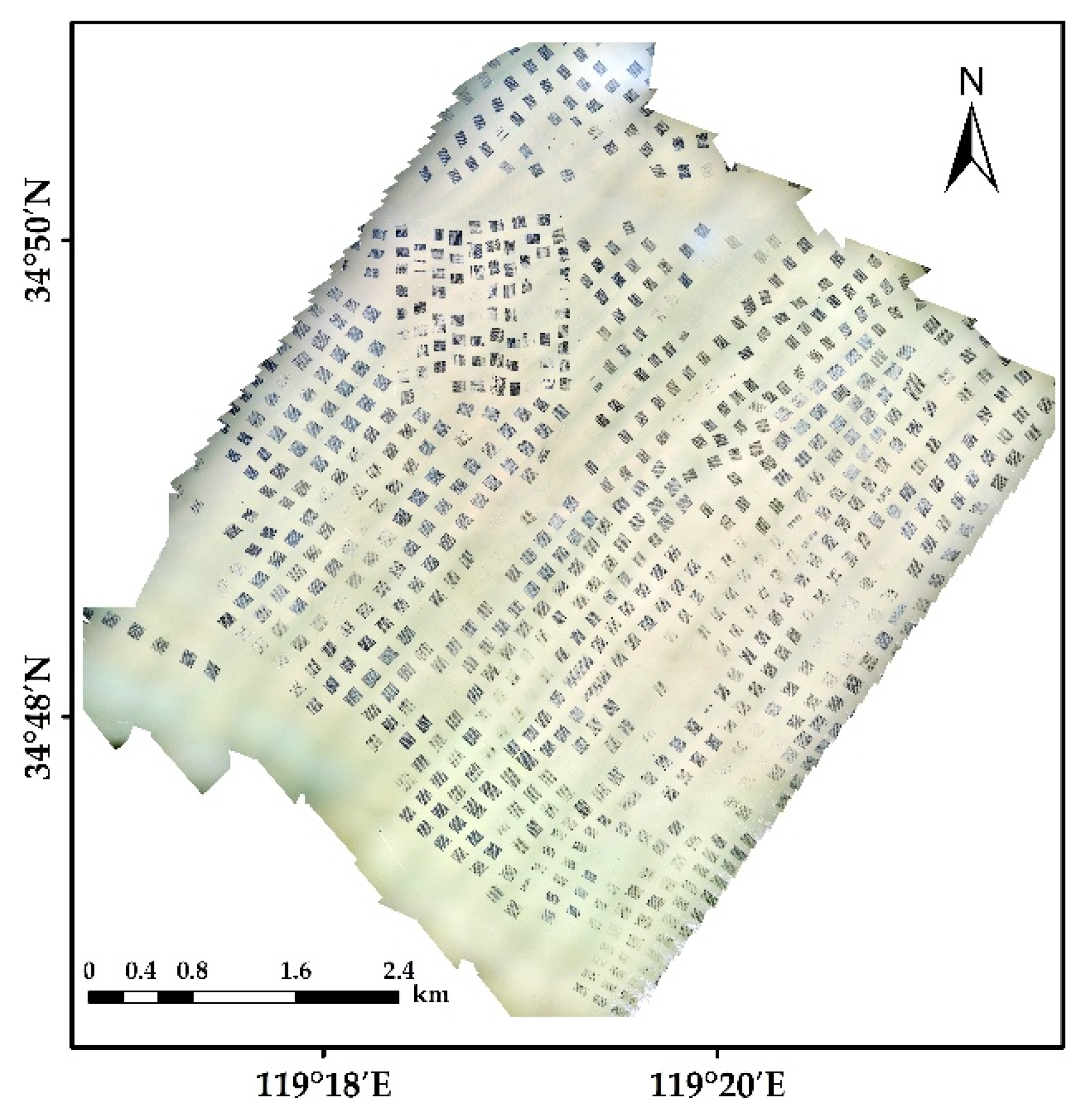
Figure 1. Remote sensing image for the experiment.
Jmse 08 00274 g001
Figure 2. Example of inaccurate supervision of classification. (a) Remote sensing image; (b) Inaccurate supervised classified image.
Jmse 08 00274 g002
Figure 3. Fully convolutional neural networks (FCN) architecture.
Jmse 08 00274 g003
Figure 4. Overall flow chart of the experiment. FCN (Fully convolutional neural network); CRF (Conditional random filed).
Jmse 08 00274 g004
Figure 5. Part of the training dataset used for model training. (a) The train images; (b) The ground truth maps.
Jmse 08 00274 g005
Figure 6. Structure of FCN-8s, FCN-16s, and FCN-32s.
Jmse 08 00274 g006
Figure 7. Results of FCN-8s, FCN-16s, and FCN-32s.
Jmse 08 00274 g007
Figure 8. The cost function curve of the FCN-8s, FCN-16s, and FCN-32s.
Jmse 08 00274 g008
Figure 9. The result of MLC (Maximum likelihood classification), SVM (Support vector machine), NN (Neural network classification), and FCN (Fully convolutional neural network). (a) Remote sensing image; (b) The ground truth map; (c) The result of MLC; (d) The result of SVM; (e) The result of NN; (f) The result of FCN.
Jmse 08 00274 g009
Figure 10. Comparison of CRF with different parameters. (a) Remote sensing image; (b) The result of FCN; (c) The result of CRF_1; (d) The result of CRF_2; (e) The result of CRF_3; (f) The result of CRF_4.
Jmse 08 00274 g010
Figure 11. Details of the results after FCN-CRF. (ac) represent remote sensing image and classification result of different regions.
Jmse 08 00274 g011
Table 1. Environmental configuration.
Software and HardwareName
Central processing unitIntel(R) Xeon(R) Gold 5118
Graphics cardNVIDIA GeForce GTX1080 Ti
Video Memory16 GB
Operating systemCentos 7
Programming languagePython
Function LibraryTensorflow, gdal, numpy, os, etc.
Table 2. Precision comparison of FCN-8s, FCN-16s, and FCN-32s.
Structure K a p p a   ( % ) P r e c i s i o n   ( % ) R e c a l l   ( % ) F 1   ( % )
FCN-8s98.4999999
FCN-16s98.0989999
FCN-32s95.2959896
Table 3. Precision comparison of MLC, SVM, NN, and FCN.
Methods K a p p a   ( % ) P r e c i s i o n   ( % ) R e c a l l   ( % ) F 1   ( % )
MLC83.3888687
SVM75.8768781
NN73.7966678
FCN98.4999999
Table 4. Confusion matrix of the classification results.
Confusion MatrixPredicted Class
Mariculture ZonesSeawaterALL
Actual classMariculture zones102,061,0261,194,492103,255,518
Seawater1,302,421374,134,673375,437,094
ALL103,363,447375,329,165478,692,612
Table 5. Parameters of the four CRF (Conditional random filed) experiments.
Parameter Name θ α θ β θ γ Epoch
CRF_150020201
CRF_2500102010
CRF_3200202010
CRF_4500202010
Table 6. Area and quantity extraction results.
Experimental ProjectArea of the Aquaculture Zone (m2)Area of the Net (m2)Number of Nets (piece)
Predicted result45,301.0425,220.451516