Article

Varying Biological Activity and Wind Stress Affect the DMS Response during the SAGE Iron Enrichment Experiment

1
Centre for Coastal Biogeochemistry, School of Environment, Science and Engineering, Southern Cross University, Lismore, NSW 2480, Australia
2
National Institute of Water and Atmospheric Research, Wellington 6241, New Zealand
3
Institute for Marine Chemistry, University of Oldenburg, 26122 Oldenburg, Germany
4
Australian Antarctic Division and Antarctic Climate and Ecosystems CRC, Kingston, Tasmania 7050, Australia
5
Southern Cross Geoscience, Southern Cross University, Lismore, NSW 2480, Australia
*
Author to whom correspondence should be addressed.
J. Mar. Sci. Eng. 2020, 8(4), 268; https://doi.org/10.3390/jmse8040268
Submission received: 12 February 2020 / Revised: 18 March 2020 / Accepted: 6 April 2020 / Published: 9 April 2020
(This article belongs to the Section Chemical Oceanography)

Abstract

:
Surface dissolved dimethylsulfide (DMS) and depth-integrated dimethylsulfoniopropionate (DMSP) measurements were made from March to April 2004 during the SOLAS Air–Sea Gas Exchange Experiment (SAGE), a multiple iron enrichment experiment in subantarctic waters SE of New Zealand. During the first two iron enrichments, chl a and DMS production were constrained, but during the third enrichment, large pulses of DMS occurred in the fertilised IN patch, compared with the unfertilised OUT patch. During the third and fourth iron infusions, total chl a concentrations doubled from 0.52 to 1.02 µg/L. Hapto8s and prasinophytes accounted for 50%, and 20%, respectively, of total chl a. The large pulses of DMS during the third iron enrichment occurred during high dissolved DMSP concentrations and wind strength; changes in dinoflagellate, haptophyte, and cyanobacteria biomass; and increased microzooplankton grazing that exerted a top down control on phytoplankton production. A further fourth iron enrichment did cause surface waters to increase in DMS, but the effect was not as great as that recorded in the third enrichment. Differences in the biological response between SAGE and several other iron enrichment experiments were concluded to reflect microzooplankton grazing activities and the microbial loop dominance, resulting from mixing of the MLD during storm activity and high winds during iron enrichment.

1. Introduction

Carbon dioxide levels continue to rise in the atmosphere, with predictions of a 1.5–2 °C increase in temperature by the end of the century [1], causing increased drought, bush fires, flooding, and sea level rise. One suggested strategy to prevent a climate catastrophe is to use iron fertilization of the ocean to stimulate phytoplankton blooms to capture atmospheric carbon dioxide. Studies have shown that natural iron fertilization during past glacial periods has repeatedly drawn up to 60 billion tons of atmospheric carbon dioxide into the ocean depths [2]. However, most of the small-scale iron fertilization experiments conducted in the recent past have not been very successful at transporting carbon to the deep ocean [1,3,4,5]. There are many reasons for this, but a major one is that it is not easy to stimulate the growth of large-cell diatoms, which seem to be needed to fix large amounts of CO2 and transport it to the deep sea. Another reason is that fertilization of the ocean with iron can also increase microzooplankton grazing, so that as soon as the CO2 is fixed by phytoplankton, it is released to the atmosphere again during the grazing of the phytoplankton.
An important secondary climate impact of iron fertilization is the production of dimethylsulfide (DMS), a trace sulfur gas produced by bacterially mediated enzymatic cleavage of dimethylsulphoniumpropionate, or DMSP, which is synthesized by ocean phytoplankton and implicated in the formation of low level clouds that can potentially lower solar radiation and sea surface temperatures [6]. The major source of cloud condensation nuclei (CCN) over the unpolluted oceans appears to be dimethylsulfide (DMS), which oxidises in the atmosphere to form a sulfate aerosol. This sulphate aerosol affects the reflectance (albedo) of clouds, and thus the Earth’s radiation budget. Charlson et al. [6] suggested that to counteract the warming owing to a doubling of atmospheric CO2, an approximate doubling of CCN would be needed, with a concomitant increase in the flux of DMS from the oceans to the atmosphere and increased formation of low level clouds.
There are many processes that affect the concentration of DMS in the surface ocean. Some of the main ones are phytoplankton cell death and bacterial decomposition to form dissolved DMSP or DMSPd, enzymatic cleavage of particulate DMSP (DMSPp) to DMSPd by DMSP-lysase and conversion to DMS by bacteria, photochemical oxidation of DMS to produce dimethylsulphoxide (DMSO), and bacterial reduction of DMSO to produce DMS [7]. Grazing can remove substantial amounts of DMSPp from the water column, and some of this may be transformed to DMSPd through cell damage during grazing (see [8]).
Several of the iron enrichment experiments carried out to date exhibit different biological responses that have affected both CO2 and DMS. For example, in the IRONEX 1 and II iron enrichment experiments, investigators observed a substantial increase in the growth of the phytoplankton assemblage to iron addition, as well as large increases in chlorophyll a, but the course of the two experiments diverged after the first three days [5]. In IRONEX I (a single iron addition experiment), the bloom did not develop and CO2 and total carbonate levels in the patch did not decline further. The whole experiment was affected by patch subduction, and it appeared that micro and mesozooplankton had responded rapidly and consumed the increased productivity of chlorophyll a by enhanced grazing [5]. In IRONEX II, where multiple iron infusions occurred, a classical “bloom” of pennate diatoms developed after the iron addition [9], resulting in further increases in chl a, a drawdown of pCO2, and decreases in silicate and dissolved inorganic carbon (DIC). The comparison of IRONEX 1 and IRONEX II provides some experimental evidence on why some areas of the ocean remove CO2 from the atmosphere because of micronutrient limitation (e.g., iron) and phytoplankton speciation (i.e., “bottom-up” control) [10], while other areas stimulate loss processes, such as zooplankton grazing (i.e., “top-down” control), and do not remove appreciable levels of atmospheric CO2 or cause increases in DMS concentrations during iron fertilization [11]
Like IRONEX II, the SOIREE mesoscale iron enrichment experiment in the polar Southern Ocean resulted in a substantial standing crop of phytoplankton, dominated by diatoms. The increased supply of iron led to elevated phytoplankton biomass and rates of photosynthesis in surface waters, causing a large drawdown of CO2 and macronutrients, and elevated DMS concentrations after 13 days. Although the bloom was slow to develop, it lasted for six weeks, indicating that recycled iron was still bioavailable [3]. An analysis of changes in DMS and intracellular DMSP (DMSPp) during IRONEX II, EisenEx, and SOIREE showed that DMSPp increased in all of the fertilized patches within four days [12,13], but the timing and depths at which maximum concentrations occurred varied between the three studies and could sometimes be related to changes in water column stability and rates of wind-driven mixing. Waters in the vicinity of New Zealand are often low in phytoplankton quantum yields (a measure of phytoplankton photosynthesis), indicative of physiological stress [14,15], making these oceanic regions an excellent area to carry out iron enrichment studies. Furthermore, the phytoplankton are often dominated by cyanobacteria [14,16,17], which are under heavy grazing pressure [18].
In this communication, we report the first continuous underway measurements of dissolved DMS concentrations, together with its precursor DMSP, in subantarctic waters SE of New Zealand sampled during the SOLAS Air–Sea Gas Exchange Experiment (SAGE), where four iron infusions were added to these waters over 15 days in 2004. SAGE was designed as a Lagrangian study, to quantify key biological and physical processes influencing the air–sea gas exchange processes of CO2, DMS, and other biogenic gases associated with an iron-induced phytoplankton bloom [8]. The aim of our part of the SAGE experiment was to ascertain what biological and physical processes affected the concentrations of dissolved DMS in the iron fertilized patch (i.e., the IN patch) compared with the unfertilized OUT patch, which were differentiated by the added chemical tracer, sulfur hexafluoride (SF6) We compared DMS, DMSP, and chlorophyll a concentrations with changes in phytoplankton speciation and microzooplankton grazing reported earlier [8,19,20], as these parameters have a major effect on DMS concentrations. Wind speed was also measured in order to ascertain the effect of variations in wind strength on dissolved DMS concentrations.

2. Methods

2.1. Site Selection

The area chosen for the iron enrichment was the Southwestern Bounty Trough, at approximately 47°0′ S, 172°0′ E (Figure 1). Following the pre-release survey, the actual first iron infusion site was selected at 46°44′ S, 172°32′ E, and this patch was followed over four weeks with three more iron infusions taking place [21]. We refer to IN stations here as the fertilised patch (i.e., IN stations, denoted by the SF6 tracer levels), and marked by a drogue. The unfertilised patches were the OUT stations (i.e., denoted by zero SF6 levels) in the continuous surface seawater samples analyzed.

2.2. The Preparation of the Iron and Dual Tracer Solutions

For iron addition, a solution was prepared from FeSO4·7H2O (containing 274 kg Fe2+) and transferred to two plastic 7500 L tanks that were initially half-filled with seawater and acidified to pH 2 by the addition of 25 L of hydrochloric acid. A total of 1.35 tons of FeSO4·7H2O was used in each infusion (Figure 2a), and the dual tracer solution was prepared in two 4000 L containers of seawater by saturation with SF6 and 3He for gas exchange studies. A headspace of ~5 L was continuously flushed with SF6 and circulated through the water via a diffusion hose and pump, until the water was saturated (Figure 2b). The iron and SF6 solutions were pumped to a depth of about 12–15 m from a pipe attached to a towed “fish” at a distance of about 20 m behind the vessel [21]. The first infusion from 15:00–23:30 (NZST = New Zealand Standard Time) on 25 March 2004 (day 0) covered about 6 × 6 km (33 km2) (Table 1) and was executed within a Lagrangian framework with an expanding hexagonal release track (with track spacings of 0.7 km), referenced to a drogued buoy at the nominal patch centre [21].
The second infusion on 31 March (00:00–06:00) of iron, SF6, and 3He took place on Lagrangian day 5.2–5.5, when the patch was described as a long filament running NNW–SSE, and thus was adapted to a compressed “lawnmower” release track of about 12 × 3 km (43 km2)(Table 1) [21] using the underway Fv/Fm signal as reference for patch location. Variable fluorescence was measured using pulse amplitude modulated fluorometry (PAM), using the saturation pulse method in order to estimate the quantum yield of photochemistry (Fv/Fm) = the ratio of the difference in the initial and maximum signal (Fv) to the maximum signal (Fm). The reduction of Fv/Fm owing to nutrient (e.g., nitrate, iron) starvation or biomass stress has been well established, and an increase in Fv/Fm is usually the first detectable response of phytoplankton to the addition of a limiting nutrient (see [19]). The third infusion on 3 April (12:30–18:30, Lagrangian day 8.8–9) was iron only, and was released in a butterfly pattern using the underway SF6 signal and occupied the second largest area (72.5 km2). The fourth infusion of iron and SF6 occurred on 6 April (22:20–03:30, Lagrangian day 12.14–12.35) (88 km2) and was released using a butterfly track with the Fv/Fm signal as reference because the dissolved SF6 concentrations were low at this stage (see [21]).
All re-infusions were successfully placed within the boundaries of the existing patch. During the site survey prior to the SAGE experiment, background dissolved iron levels were low at ~0.10 nM. After the first infusion, dissolved iron concentrations ranged from 0.14 to 3.03 nM (mean 1.27 ± 0.82 nM) and dropped to an average value of 0.2 ± 0.09 nM. The second infusion raised dissolved iron levels to a maximum of 1.59 nM and, by 2 April, they had decayed to a level of about 0.1 nM in two days. After the third infusion, maximum iron concentrations were 0.55 nM. Finally, the fourth infusion resulted in a decline from a high of 1.01 nM to 0.32 nM just prior to leaving the patch site (Table 1).

2.3. Wind Speed and SF6 Mapping

Wind speeds were obtained from an automatic weather station (AWS), maintained and calibrated by the Meteorological Service of New Zealand. It was located at 25.2 m above sea level, above the crow’s nest and bridge of the Tangaroa, which exposed it to all wind directions. The AWS wind data were compensated for ship translational motion and logged at 5 min intervals on the ship’s data acquisition system. Wind speeds were measured under a range of atmospheric stability conditions and were corrected to neutral stability and to 10 m equivalent height (U10).
SF6 mapping began 3 h after the end of the first iron infusion at 02:30 NZST on 26 March (D1) (Table 1), with associated underway surface measurements of temperature, salinity, chlorophyll fluorescence, Fv/Fm, and current velocity using an Acoustic Doppler Current Velocity profiler (ADCP) [21]. Surface water from 7 m depth was continuously sampled with dissolved SF6 stripped, cryogenically trapped, and detected by an ECD-gas chromatograph every 3 min (see [21]). Surface mapping took place between 21:00 and 07:30 each day, in which the IN station location was identified by the SF6 concentrations.

2.4. Phytoplankton Pigments

Phytoplankton pigment samples were collected by filtering seawater from the CTD cast under low pressure through 13 mm glass fibre (GF/F) filters and storing them in liquid nitrogen until extraction by sonication for 1 min in 1.5 mL methanol with 140 ng apo-8-carotenal (Fluka, internal standard) back at the shore laboratory [22] and analysis by high performance liquid chromatography using the method of [23]. The results have been reported in Peloquin et al. (2011 a) [19] and are included in new figures here in order to examine correlations between DMS and DMSP. Statistical testing was computed with time using linear trend analysis (p < 0.5) (see [19]). Paired stations were compared using Student’s t-test. Pigment data were examined using PATN software, comparing IN and OUT stations as a priori groups, that is, those with high or low concentrations of SF6 in samples, similar to our DMS analysis in Table 2 [19].

2.5. Microzooplankton Grazing

Microzooplankton grazing experiments were carried out at 21 stations and comprised 15 IN stations and six OUT stations on CTD casts. Water was collected using a Seabird (SBE-9 plus) CTD and rosette from approximately 7–12 m depth. The main findings of these results have already been presented [20], but are included in new figures here, alongside our DMS results, as production and consumption of DMSP can be significantly affected by microzooplankton grazing, which in turn affect DMS concentrations in Sub-Antarctic waters [7].

2.6. Underway DMS Measurements

From 24 March (23:30) to 15 April (08:30), a seawater sample was collected from the ship’s underway system from 7 m below the sea surface and analyzed for dissolved DMS every 14 min with an automated purge and trap gas chromatographic system designed by Mike Harvey and John McGregor (NIWA). The seawater was pumped through a plastic hose to the gas chromatography (GC) lab below deck of the RV Tangaroa and filtered through a Gelman extra thick glass fibre filter (25 mm diameter and pore size of 1 µm), contained in a polycarbonate filter assembly. The filtration system contained ten such filters and, after a pre-determined time, a computer switched filtration to the next filter. The samples were filtered at 20 mL/min. In order to prevent the build-up of phytoplankton on the filter, the filtration time was reduced from 120 min to 60 min after the first two iron enrichments. Filtered seawater (12 mL) was introduced into a 50 mL glass purge chamber every 14 min via a computer activated valve. The dissolved DMS was purged from the seawater with oxygen-free nitrogen into a cold trap, consisting of a thin Pyrex tube containing Tenax TA that was cooled to −20 °C with ethylene glycol. After 10 to 12 min of purging, a pump stopped circulating the glycol and DMS was thermally desorbed from the trap at 120 °C and injected into a Varian 3400 GC fitted with a pulsed flame photometric detector (PFPD). The sampling, purging, desorption, and gas chromatography were fully automated using a Lab VIEW control system. DMS in IN or OUT stations was identified by the SF6 concentration approximately every 25 min.
An inter-calibration of dissolved DMS on CTD cast 538 was carried out on 24 March at the start of the voyage using the automated GC technique and a manual GC technique employed mainly for DMSP production and consumption studies [24]. The results by both techniques agreed to within 0.1 nM of DMS (see data report).
A comparison of underway dissolved DMS concentrations by the two techniques later in the voyage on 2 April (Lagrangian day 8) gave higher values for the automated technique. Consequently, an inter-calibration factor was applied to the underway data. The difference only lay in the deviation of the intercept, possibly reflecting some loss of sensitivity in the automated method when a new Tenax tube had to be conditioned earlier. During Lagrangian day 8, and prior to the third iron enrichment, continuous underway DMS concentrations (automated method) in the OUT patch ranged from 0.09 to 0.73 nM (mean = 0.46, n = 20) (Table 2), while the manual GC method gave DMS concentrations ranging from 0.52 to 0.66 nM (mean = 0.59 nM, n = 4) [24]. A difference of 0.13 nM DMS was closely similar to the results of the first intercalibration exercise. Blanks were non-detectable. Precision was ±10% on the replicate analysis of seawater.

2.7. Surface Seawater DMSP Concentrations

In seawater, DMSP is operationally divided into two fractions, the intracellular or particulate (DMSPp) form in phytoplankton, which is retained by filtering seawater through a 0.45 µm filter [25,26], and an extracellular or dissolved (DMSPd) form, which passes through the filter. The relative ratios of DMSPp to DMSPd and DMS are influenced by the various life stages of the phytoplankton and zooplankton community, and the composition of the microbial food web. DMSPp in phytoplankton can be converted to DMSPd by DMSP enzymes from grazing activities and bacteria. Samples for DMSP analysis were taken from the CTD rosette in the upper 90 m of the water column at “IN patch” and “OUT patch” stations. Unfiltered samples for DMSP analysis were stored in 100 mL acid-rinsed amber glass bottles for total DMSP (DMSPt) and acidified with HCl to pH < 2. DMSPd samples were gently syringe filtered (0.45 µm, Millipore), drop by drop, prior to acidification.
Deschaseaux et al. (2014) [27] compared 0.45 μm polycarbonate syringe filtration of seawater using a drop by drop technique to samples that filtered by gravity filtration through GF/F filters [28]. Deschaseaux et al. have shown that DMSPd concentrations are on average 54.5% lower (p < 0.001) than gravity filtered samples when seawater is carefully hand-filtered through 0.45 μm Millipore filters. The averaged coefficient of variation (CV) for both treatments was 17.9% for hand filtration versus 15.3% for gravity filtration. These results suggested that either (i) small cell phytoplankton containing some DMSPp could pass through GF/F filters (0.7 μm mesh), but can be removed using smaller pore size (0.45 μm) syringe filters; (ii) more DMSPp was drained out of algal cells by gravity filtration compared with hand-filtering; or (iii) the difference in filter material (glass fibre versus polycarbonate) could be because polycarbonate filters have very regular pores, while glass fibre filters are a mesh of irregular sized spaces. Ultimately, as lower DMSPd concentrations were obtained by hand-filtering with 0.45 μm syringe filters, it was concluded that this technique allows for a finer separation of the DMSPd fraction from DMSPt [27]. This method was thus used in this experiment.
Measurements of DMSPp, DMSPd, and DMSPt concentrations were obtained on filtered seawater after alkali cleavage to DMS and gas chromatography analysis [26,29].

3. Results

3.1. SF6 Mapping and Dissolved Iron

Concentrations of SF6 were initially ~400 fmol/L, but declined on Lagrangian day 2 to ~40 fmol/L following high winds and increased air–sea exchange, as well as dilution from deepening of the mixed layer [21]. Following the second infusion on Lagrangian day 5.2–5.45, SF6 levels were again ~400 fmol/L on Lagrangian day 6, and slowly decreased to <50 fmol/L on Lagrangian day 12. A lateral intrusion caused the SF6-labelled water to shoal to <40 m from Lagrangian day 6 and between Lagrangian days 6 and 9 was characterized by two mixed layers (22–30 m and 34–87 m), an increase in nutrients, a minor decrease in Fv/Fm, and a significant decrease in chl a [8]. Maximum lateral intrusion occurred on Lagrangian day 7.5, during which low salinity water extended up to 20 m. Law et al. (2011) [21] state that this intrusion most likely originated from Sub-Antarctic water drawn up from the south, along the eastern face of the Southland Current [30]. The third infusion (Table 1, Lagrangian day 8.75–9) was an iron solution only with appreciable SF6 levels (>10 fmol/L). The fourth infusion of SF6 and iron was released on Lagrangian day 12.14–12.35 using an adaptive track with the underway Fv/Fm signal as a reference [8]. Pre-infusion dissolved Fe in surface waters was 0.12 ± 0.04 nM, with subsequent surface sampling outside the patch with a background dissolved Fe of <0.09 nM [21]. The first infusion raised Fe levels to 3.03 nM. The second, third, and fourth infusions raised Fe to 1.59, 0.55, and 1.01 nM, respectively (see Table 1).

3.2. Total Chlorophyll a and Photosynthetic Efficiency (Fv/Fm)

In the IN patch total chl a in surface waters showed a slight increase from Lagrangian days 2 to 5 (0.50–0.59 µg/L), a steeper increase from Lagrangian days 5 to 7 (0.59–0.80 µg/L), followed by a marked drop in chl a concentrations on Lagrangian day 8 to 0.52 µg/L (Figure 3a). From Lagrangian days 8 to 15, during the third and fourth iron infusions, total chl a concentration increased from 0.52 to 1.02 µg/L (Figure 3a). Total chl a concentrations in surface waters of the OUT patch (Figure 3b) averaged 0.58 µg/L (range 0.44–0.86 µg/L; n = 13) throughout the 15 days of the experiment. Total chl a thus doubled in concentration over the course of the experiment in the IN patch (Figure 3a,b). Law et al. [21] found that periods of elevated chl a occurred when dilution was less than the phytoplankton growth rate, during Lagrangian days 3–6 and days 10–14.
Fv/Fm increased from an average value of 0.26 in the patch during the night of day 0, to 0.35 by the night of Lagrangian day 4, and was 0.06 higher than the surrounding water, indicating a definite physiological response by the phytoplankton community to the increased iron availability [8]. Following the third and fourth iron enrichments of the patch, Fv/Fm rose from about 0.32 on Lagrangian day 9 to an average of 0.38 on the night of Lagrangian day 13 (0.45 in parts of patch).

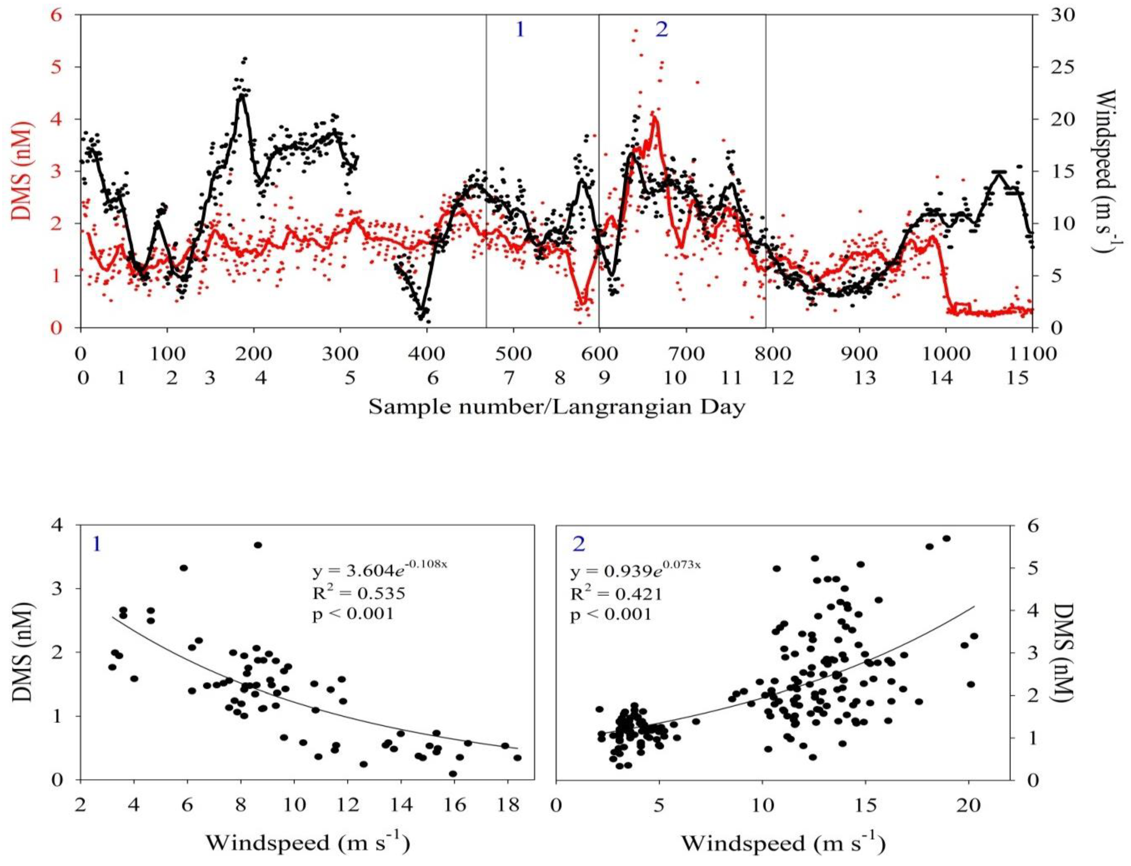
3.3. Continuous Underway Dissolved DMS Concentrations

A comparison of continuous DMS concentrations (n = 1100) in surface seawater of the IN patch with the those of the OUT patch surface waters revealed no significant differences until after the third iron enrichment (Figure 4a,b). On Lagrangian day ~8, mean dissolved DMS concentrations were quite low, at about 0.46 nM (range 0.09–0.73, n = 20) in the IN patch (Table 2, Figure 4a).
The third iron infusion occurred from 12:30 to 18:30 on 3 April (Table 1)) and no tracer was added as reasonable concentrations of SF6 were still detected (10–34 fmol/L) (Table 2). From 10:55 on Lagrangian day 9 to 12:30 on Lagrangian day 10, dissolved DMS concentrations increased markedly in the IN patch (Figure 4a) and ranged from 1.12 to 5.7 nM (mean 2.69 nM, n = 72) (Table 2), and were significantly higher than mean DMS concentrations measured in the OUT patch on Lagrangian day 10 (12:45–18:10) (range 0.54–1.91 nM, mean 1.27 nM, n = 12) (p < 0.05) (Table 2 and Figure 4b). From 18:45 on Lagrangian day 10 to 02:40 on Lagrangian day 11, underway DMS concentrations in the IN patch were again higher than OUT patch measurements on Lagrangian day 11 (range 0.81–4.7 nM, mean = 2.21 nM, n = 25) (Table 2). During the morning of Lagrangian day 11 (04:45–10:35), DMS concentrations in the IN patch were still elevated (range 1.42–3.59 nM, mean 2.25 nM, n = 18), comparable to IN patch measurements made on Lagrangian day 10, and early on during Lagrangian day 11 (mean 2.21 nM). However, thereafter, from Lagrangian days 11 to 14, IN patch mean DMS concentrations were much lower (mean = 1.3–1.4 nM, n = 65) (Table 2). Diurnal variations in DMS concentrations were apparent during the third iron enrichment. For example, the very high concentrations of DMS often occurred in the late afternoon to early morning when tracer and iron was added to the IN patch (Table 2).
During the fourth infusion on Lagrangian day 12, underway DMS concentrations increased slightly over OUT patch measurements, but no significant difference between the IN and OUT patch occurred, and by Lagrangian day 14, underway DMS concentrations in the IN patch were very low (mean 0.3 nM, n= 19), and comparable to concentrations measured on Lagrangian day 8 prior to the third iron enrichment (Table 2). When we compare these DMS results (Figure 4a,b, Table 2) with those reported by Archer et al. (2011) [24] for the same voyage, we see that the discrete sampling of Archer et al. missed the pulse of elevated dissolved DMS in the IN patch from Lagrangian days 9 to 11 during the third iron enrichment, perhaps owing to the bad weather and low sample coverage at that time. We note that the DMS concentrations reported by Archer et al. (2011) [24] are for the averaged mixed layer or inferred mixed layer depths (ranging from 30 to 75 m). Archer et al. (2011) [24] found MLD integrated values for the fertilised IN patch were all <1 nM (n = 13) with sampling more widely dispersed during the experiment. However, it is clear from our continuous DMS measurements in surface waters that there are occasions when our lower concentrations of seawater DMS (Figure 4a) were comparable to those of Archer et al. (2011) [24].

3.4. Wind Speed and Correlation with Seawater DMS Concentrations

Wind speeds varied appreciably during the experiment, ranging from 1 to 26 m s−1 (2–50 knots), providing an excellent basis to assess the response of DMS concentrations. The response varied through the experiment. For the first six days, there was no obvious correlation between DMS (which ranged from ~0.5 to 2 nM) and wind speed, despite the latter encompassing the full range of the experiment (Figure 5).
After the second iron infusion (Table 1), from approximately Lagrangian day 6.8 to 8.7 (Period 1), DMS decreased as wind speed increased (r2 = 0.54, p < 0.001). Just prior to the third iron enrichment (Table 1), DMS concentrations and wind speed were anti-correlated with DMS concentrations, reaching a low of 0.46 nM as wind speed reached 18 m/s. A sharp, almost vertical increase in WS to ~18 m s−1 occurred on Lagrangian day 9–10, which quickly dissipated to 2 m s−1 by Lagrangian days 11–12. It was during this period (Period 2) that seawater DMS concentrations displayed four pulses of elevated DMS concentrations (Figure 5), suggesting that biological production of DMS in iron enriched surface waters was keeping up with the diluting effects of increased wind stress and sea–air gas exchange and displaying a highly significant positive correlation with wind speed (r2 = 0.42, p < 0.001).

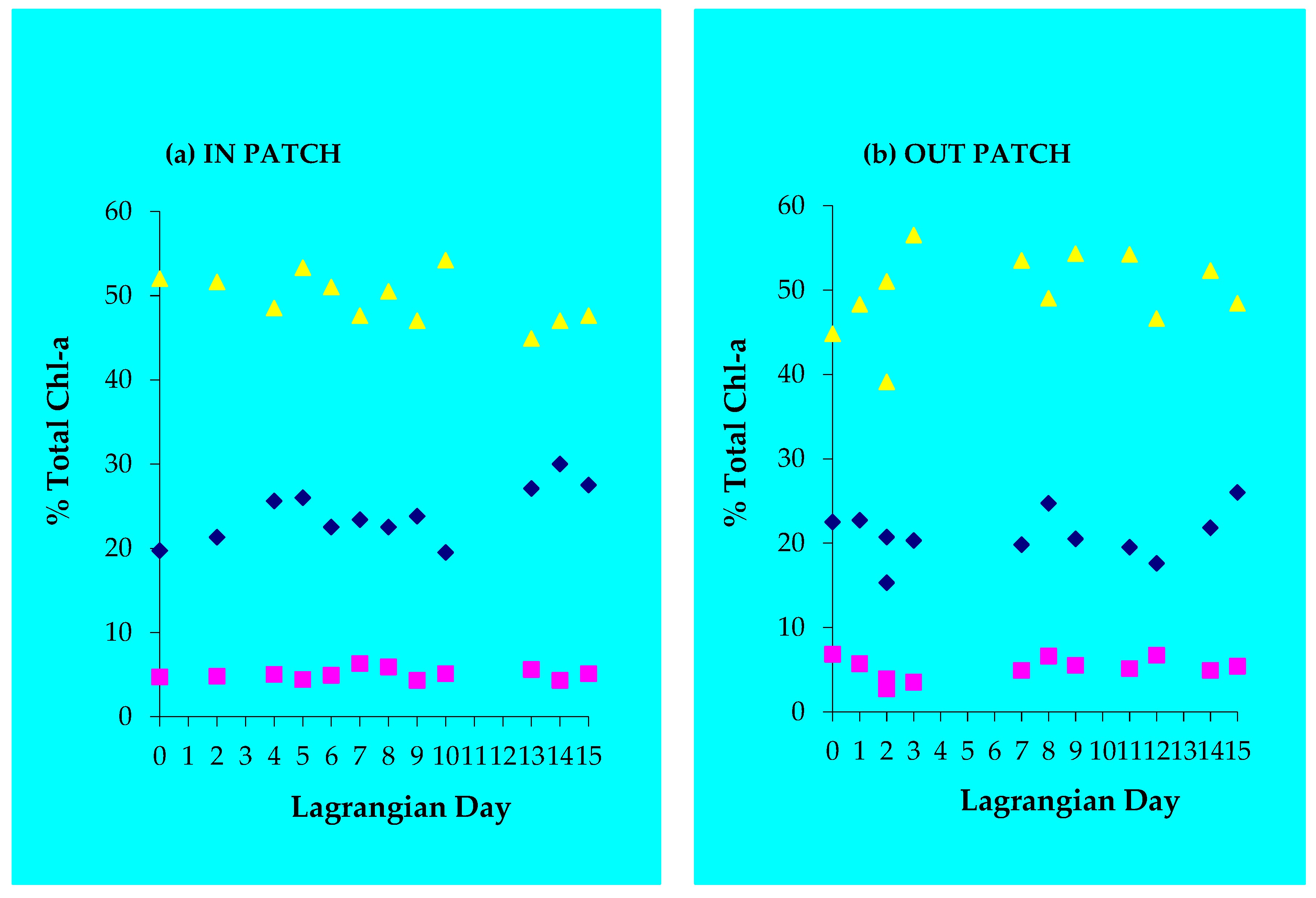
3.5. Variation of the Depth-Integrated DMSP and Chl a Fractions

Seawater samples (n = 187) from the CTD casts were analyzed for all fractions of DMSP and chl a ranging from depths of 0–90 m, spanning the pre-fertilization period, patch surface monitoring, and comparisons of inside and outside the enriched patch. On a mean basis, very little difference occurred between IN patch and OUT patch measurements of the different DMSP fractions. For example, depth-integrated DMSPt concentrations of IN patch versus OUT patch averaged 45 nM (21–69 nM) vs. 41 nM (32–50 nM), respectively; DMSPp concentrations averaged 13 nM (7–26 nM) vs. 14 nM (11–15 nM), respectively; DMSPd concentrations averaged 33 nM (9–62 nM) vs. 27 nM (18–38 nM), respectively; and surface chl a averaged 0.76 µg/L (0.51–1 μg/L) vs. 0.58 µg/L (0.44–0.86 µg/L), respectively. When the DMSPt, DMSPp, and DMSPd fractions are plotted against Lagrangian day for the IN patch, both DMSPt and DMSPd sulfur fractions showed the same patterns of decreasing and increasing concentrations with the largest increase of both sulfur fractions occurring between Lagrangian days 6 and 15 (Figure 6a). Depth integrated DMSPp concentrations in the IN patch generally decreased over the course of the experiment (Figure 6a). Conversely, surface chl a showed one peak in concentration from Lagrangian days 4 to 10 (highest concentrations on day 7 and 8) and a second peak in chl a from Lagrangian days 10 to 17 (highest concentration on day 16) (Figure 6b).

3.6. Phytoplankton Pigments

Factors controlling phytoplankton growth, biomass accumulation, primary productivity, and grazing during the experiment have already been described [19,20]. Pigment analysis of surface waters indicated that the most abundant group was Hapto8s (cells with pigmentation typical of Type 8 haptophytes (e.g., Phaeocystis sp. and Pelagophytes)) [31]. Relative abundances were as follows: Hapto8s > Prasinophytes > Chlorophytes > Dinoflagellates > Cyanobacteria > Cryptophytes, with hapto8s accounting for about 50% of the total chl a, prasinophytes for just over 20%, and all other groups for 30%. Pigment analysis indicated that diatoms were negligible in both the IN and OUT patches, with the fucoxanthin (FUCO) to chl a ratios averaging 0.07, which included the contribution from haptophytes. In the IN patch, hapto8s decreased slightly, while prasinophytes increased from 20% to 30% of total chl a, and dinoflagellates did not change (Figure 7a). Cyanobacteria in the IN patch seemed to decrease from Lagrangian day 0 to day 9, with no discernible trend in chlorophytes and cryptophytes (Figure 7c). In the OUT patch, surface waters cyanobacteria and dinoflagellates seemed to increase from about Lagrangian day 2 to 4, while there was no trend in the chlorophytes (Figure 7d). Compared with trends in the OUT patch, there only seemed to be a significant IN patch change for prasinophytes (Figure 7a). While no significant changes seemed to occur with most other phytoplankton assemblages (as determined by CHEMTAX pigment analysis) (Figure 7a–d), significant changes occurred in a low seed stock of diatoms determined by microscopy. Although the very low seed stock of diatoms represented <1% of the recorded biomass [8], these authors describe a consistent increase in this diatom seed stock from Lagrangian day 3 (~0.013 µgC/L) to Lagrangian day 9 (~0.072 µgC/L), and then a sharp drop in diatom biomass on Lagrangian day 10 (~0.025 µgC/L). Diatom biomass then increased slightly on day 12 (~0.035 µgC/L), decreased again on Lagrangian day 14 (~0.008 µgC/L), and then increased to ~0.06 µgC/L on Lagrangian day 16. On the basis of absolute pigment concentrations, only the typical prasinophyte pigments were statistically different for the IN and OUT patch [19]. These authors further state that all of the minor prasinophyte pigments’ (but not chl b) concentrations responded strongly and immediately to the addition of iron.

3.7. DMSP Pigment Correlations

There were significant correlations between IN patch depth-integrated DMSPt concentrations (surface 90 m) and depth-integrated total chl a and fucoxanthin (FUCO, a significant pigment in diatoms and most haptophytes); 19′-hexanolyoxyfucoxanthin (HEX, a significant pigment in types 6–8 haptophytes, including coccolithophorids and Phaeocystis, Pelagophytes, and some dinoflagellates); peridinin (PERI, an unambiguous marker for type 1 dinoflagellates); and β, β- carotene (a common accessory/photoprotective pigment) (Table 3). However, depth-integrated correlations between DMSPp and phytoplankton pigments were weak (Table 3).

3.8. Dominant Phytoplankton Species, Growth Rates, and Microzooplankton Grazing

Prasinophytes, dinoflagellates, and haptophytes are all significant producers of DMSP [32]. When potential contributions of chlorophyll a from these three dominant phytoplankton assemblages or CHEMTAX groups in surface waters (i.e., FUCO, PERI, HEX) are considered as a percentage of total chl a, and are plotted against Lagrangian day, it can be seen that the percentage of chlorophyll a in all three assemblages decreased in the IN patch on Lagrangian day 7 (10%) after the second enrichment, and a drop of 12% in surface waters during the third enrichment on Lagrangian day 10 can also be observed (Figure 8a). After Lagrangian day 10, all three phytoplankton assemblages slowly increased from a low of 71% to 83% of total chlorophyll a on Lagrangian day 13, a day after the fourth enrichment. These three phytoplankton assemblages then decreased to 77% on Lagrangian day 14, before increasing to 92% on Lagrangian day 16 as we left the area (data not shown). In contrast, in the OUT patch, total chlorophyll a steadily increased over the 15 days. The relationships between our DMS concentrations and microzooplankton grazing pressure are shown in Figure 8c,d. These show that the peak concentrations of DMS at Day 10.6 and subsequent fall occurred when the ratios of phytoplankton growth to microzooplankton grazing were generally close to 1, but generally less than 1 for cells in the <2 µm fraction (Figure 8c) with a relatively steady increase in the microzooplankton biomass (Figure 8d).

4. Discussion

4.1. Chlorophyll a and Phytoplankton Pigments

During the first two iron enrichments, chl a and DMS production was constrained with little difference in DMS concentrations in surface seawater from the IN and OUT patch (Figure 4a,b). However, during the third iron enrichment, during Lagrangian days 9–11, large pulses of dissolved DMS concentrations occurred in the fertilised IN patch as chl a increased. This did not occur in the unfertilised OUT patch surface waters (Figure 4b). The question we have to ask ourselves is what physical and biological processes caused these very high concentrations of DMS during the third iron enrichment. Over the course of the 15 day experiment, hapto8s in the IN patch tended to decrease slightly in abundance, while cyanobacteria decreased to Lagrangian day 9, likely a result of increased microzooplankton grazing [19,20]. Cyanobacteria then increased as a percentage of total chl a to Lagrangian day 16 (Figure 7b,c), prasinophytes increased slightly in the IN patch, and dinoflagellates biomass was constant throughout the experiment in both IN and OUT surface waters (Figure 7a,b). On the basis of absolute pigment concentrations, only the typical prasinophyte pigments were statistically different from inside and outside the patch (p < 0.05). All of the minor prasinophyte pigments (not chl b) concentrations responded strongly and immediately to the addition of iron (see [19]). There was no obvious trend in chlorophytes and cryptophytes in both IN and OUT waters (Figure 7c,d).
Haptophytes, prasinophytes, and dinoflagellates are all significant producers of DMSPp, while cyanobacteria are not [32]. When potential contributions from haptophytes, prasinophytes, and dinoflagellates (i.e., CHEMTAX pigments FUCO, PERI, HEX) are considered as a percentage of total chl a and are plotted against Lagrangian day, it can be seen that, in the OUT patch, all three phytoplankton assemblages increased (Figure 8b), while in the IN patch, these three phytoplankton assemblages generally increased during/after the iron additions (Figure 8a). The large decreases in chl a at Lagrangian days 7 and 10 could have reflected increased microzooplankton grazing on chl a as a result of increased iron addition, and increased mixing by high wind speeds (Figure 5).
DMSPt was significantly correlated with all pigments, but most significantly correlated with FUCO, PERI, and β, β- carotene (p < 0.01) (Table 3). DMSPp was not significantly correlated with any pigments in the IN or OUT patch. β, β-carotene is not a taxonomic marker, being a widespread photoprotective pigment. In an iron-depleted algal community in the Peru, upwelling of β, β-carotene correlated strongly with DMSPp and DMSOp and it was suggested that the pigment acted as an antioxidant under iron stress [33]. We also observed a strong correlation of β, β-carotene with DMSPt (r2 = 0.77) over Lagrangian day during SAGE, which could suggest that phytoplankton were subject to some constant stress (e.g., grazing) during the experiment, which increased DMSPd concentrations (Table 4).

4.2. Microzooplankton Grazing

Studies of natural phytoplankton blooms have measured increased DMSPd concentrations owing to grazing [34,35,36,37,38] During the SAGE experiment, the heterotrophic nanoflagellate (HNF) population was composed of colorless dinoflagellate species and Kinetoplastidae contributing approximately equal proportions of the total microzooplankton biomass [20]. Heterotrophic dinoflagellates observed included Protoperidinium spp., Diplopsalis sp., and Gyrodinium spirale, with a number of other species including some Gymnodinium spp., Amphidinium spp., and c.f. Oxytoxum spp. [20]. The phytoplankton >20 µm size fraction was dominated by dinoflagellates, which were potential grazers of chl a. The biomass of HNF and ciliate microzooplankton trended upwards from a low at the pre-infusion stage, peaked on Lagrangian day 5, and slowly increased from Lagrangian days 6 to 10, remaining fairly constant from Lagrangian days 11 to 15 [19].
In the shipboard microzooplankton grazing experiments carried out by [20], grazing rates in the <200 µm, <20 µm, and <2 µm size fractions were usually greater than the phytoplankton growth rates (see Table 1) [20], and from Lagrangian days 8.6 to 9.6, microzooplankton grazing rates increased 50% in the two smallest size fractions. Peloquin et al. [20] state that microzooplankton grazing could consume 15%–49% of the total phytoplankton production per day, with removal highest on eukaryotic picophytoplankton production (mean 72%, range 29%–143%) in the <2 µm fraction. Microzooplankton biomass doubled over the course of the experiment, as a result of an increase in cell size [20], possibly a result of iron enrichment and grazing selectivity. These authors reported the ratio of phytoplankton growth rates to grazing rates (d−1) for the three different size fractions over the experiment [20]. Plotting these ratios (µ/g) from Lagrangian days 0 to 5, we see that for the <20 µm fraction, the ratios are >1, suggesting that phytoplankton growth rates are higher than grazing rates (Figure 8c). However, from Lagrangian day 5.6 to 12.6, the <2 µm ratios are often <1, indicating that grazing rates are increasing over phytoplankton growth rates. From Lagrangian days 1 to 11, mean seawater DMS concentrations ranged from 0.5 nM to 4.5 nM (Figure 8c), and microzooplankton biomass significantly increased over this period (Figure 8d). The increase in microzooplankton biomass was significant (p < 0.05) when a linear regression fit was applied to the heterotrophic nanoflagellates (HNF) and ciliate biomass data separately (i.e., <2 um fraction), which gave r2 values = 0.3 and 0.42, respectively, and as a whole (r2 = 0.68). The fitted slope suggested that microzooplankton biomass increased by ~2.3× or 230% over the patch occupation [20].
When phytoplankton production of chl a was greater than microzooplankton grazing (Figure 8c), it may have caused the two peaks in depth-integrated chl a concentrations during the iron enrichment (Figure 6b). The first peak occurred during days Lagrangian days 0–6, when the first two iron enrichments occurred, with a rapid and more sustained increase from Lagrangian days 6 to 10 during the third iron enrichment. From Lagrangian days 10 to 15 (which included the fourth iron enrichment), chl a consistently increased (Figure 6b). DMSPp accumulation was suppressed in part by microzooplankton grazers, who consumed between 61% d−1 and 126% d−1 of the DMSPp production. In turn, DMSPd production increased significantly from Lagrangian days 6 to 15 (Figure 6b), so it is possible that phytoplankton growth was stimulated during the third iron enrichment, but was immediately grazed, causing DMSPp concentrations to decrease (Figure 6a). This would have kept chl a relatively low, while DMSPd concentrations increased. Davey and Geider (2001) [39] found that, upon alleviating iron stress, phytoplankton allocate the micronutrient for biochemical reactions before cell division. This may explain the slower increase in chl a during SAGE (Figure 6b).
Microzooplankton grazing rates in the <2 µm fraction were in balance with phytoplankton growth rates on Lagrangian day 9.6, but on Lagrangian days 10.6 and 12.6, grazing rates were five times and two times the phytoplankton growth rates, respectively [19]. This did not occur for the <20 µm and <200 µm fractions. This increased grazing activity coincided with increasing microzooplankton biomass and the highest mean surface seawater DMS concentrations on Lagrangian day 10.6 (Figure 8d). We believe the key biological processes that elevated DMS concentrations around Lagrangian days 9–12 were microzooplankton grazing, which elevated DMSPd concentrations, and the conversion to DMS by higher rates of bacterioplankton production in the iron enriched waters at the surface from approximately Lagrangian day 10 [40,41].

4.3. Effect of Increasing and Decreasing Wind Speed on Dissolved DMS

Increasing wind speed can have at least two effects on dissolved DMS concentrations. Firstly, as wind speed increases, it can increase the exchange of dissolved DMS with the atmosphere and deplete the surface of the ocean of dissolved DMS. This occurs after the first iron enrichment on 25 March (approximately Lagrangian day 0–1, Figure 5), and mainly from the 26 March to 31 March period (Lagrangian days 1–5.5), when DMS very slowly increased, prior to the second iron enrichment (Figure 5). A short decoupling of wind speed and DMS occurred on 3 April (Lagrangian day ~8.5) (Figure 5). From 3 April to 5 April (Lagrangian days ~9–11), at least four large increases in DMS concentrations occurred as wind speed increased and decreased, indicating a close coupling between both parameters after the third iron enrichment on 3 April (Table 1). There was also a close coupling between wind speed and DMS from 6 April to 8 April (Lagrangian days 12–14) after the fourth iron enrichment on 6 April. From 9 to 10 April, the two parameters decoupled, when Tangaroa headed for the Southern Mooring and travelled through completely different waters to the study site. To roughly estimate DMS gas exchange for period 1, there was a decrease in DMS of ~2 nM (i.e., 2.5 nM minus 0.5 nM) (see Figure 5) over two days as wind speed increased, indicating a gas exchange of DMS of 0.04 nM h−1 from the sea surface as wind speeds went from 2 to 18 m s−1. DMS production rates during iron enrichment were estimated in period 2 from days 9 to 10 (~24.5 h, Table 2) when there was a marked increase in DMS to about 5.7 nM (red line, Figure 5). DMS concentrations went from 1.12 nM to 5.7 nM (i.e., an increase of 4.6 nM (Table 2)), giving a production rate of +0.19 nM DMS hr−1 over a much shorter period of time. From day 10 to 12, DMS concentrations slowly decreased from 5.7 nM to 1.29 nM (Table 2), a decrease of 4.3 nM over about two days, giving a consumption rate of 0.09 nM h−1.
Increasing wind speed increases the depth of the mixed layer (i.e., more mixing occurs between surface waters and deeper waters), which can have a significant effect on dissolved DMS concentrations because it can increases nutrients concentrations in the surface layer of the ocean. The depth of the mixed layer can vary markedly because of the wind strength. During the third enrichment, we believe the marked increase in DMS concentrations may have reflected an increased supply of nutrients from the mixed layer to surface waters from the increased wind speed and increased biological activity, causing a short, but rapid increase in seawater DMS concentrations, aided by increased iron supply. An intrusion of surface OUT patch water into the IN patch, aided by wind mixing, can also not be discounted [42,43].

4.4. Comparison of DMS (P) with Other Iron Enrichment Experiments

IRONEX II in the equatorial Pacific produced high dissolved DMS concentrations quite early in the experiment at day 6, which was a much quicker response than recorded in SOIRE, EisenX, and SAGE (Table 4). In the Southern Hemisphere experiments, increases in dissolved DMS occurred from Lagrangian days 10 to 13 (Table 4), similar to our results. These differences reflect different biological responses during iron enrichment. For example, during IRONEX I, picophytoplankton and dinoflagellates dominated the algal community [44]. Diatoms, which were not heavily grazed, were dominant during IRONEX II, while picophytoplankton populations only slightly increased [9]. SOIREE in the Southern Ocean also saw a change in dominance from picophytoplankton to diatoms, however, prymnesiophyte abundance also increased ahead of the diatom domination, which increased DMSP and DMS production by stimulating grazing [3,45]. Enhanced grazing during SAGE also explains our elevated DMS results during the third enrichment. For example, IN patch prasinophytes, dinoflagellates, and hapto8s (as % of total chl a), which would increase DMSPt, decreased markedly after the second and third enrichments, probably from increased grazing (Figure 7b). This may have constrained the production of chl a, whereas these three phytoplankton assemblages increased in the OUT patch over the course of the whole experiment (Figure 8b).
At the beginning of SAGE, DMSPp concentrations were closest to IRONEX II and generally lower than starting concentrations from other experiments (Table 5). Similar to SAGE results, DMSP concentrations during SOIREE increased from Lagrangian day 3 owing to increased grazing [3]. DMSPp concentrations decreased from the beginning to the middle of SAGE, while all other experiments showed large increases in response to iron additions (Table 5). On Lagrangian day 16 of SAGE, depth-integrated DMSPp was 37 nM, which fit the trend of previous experiments and was closest to ending concentrations for SOIREE. Turner et al. (1996) [11] reported similarly that DMSPp showed a second maximum during IRONEX II on day 13, which was surrounded by lower concentrations. They suggested that the lower concentrations were the result of physical mixing and dilution of the experimental patch, rather than decreased biological production. However, these results could also have reflected an increase in nutrients, which stimulated chl a and DMSPp production, which in turn stimulated grazing (see [46]). A reanalysis of results for the IRONEX experiments with SOIREE and EisenEx suggested that the warm water communities of the Pacific were able to increase DMSPp production almost immediately, whereas in the Southern Ocean, there was a delay with an initial loss of DMSPp [12]. These authors also hint at two cycles in DMSPp levels with a periodicity of about 10 days, which they suggest indicates predator–prey dynamics involving the microbial loop [46] and grazing [47].
Studies of natural phytoplankton blooms have measured increased DMSPd concentrations owing to grazing, which then decrease owing to bacterial or viral conversion to DMS and other sulfur compounds [34,35,36,37,38]. In SAGE, as the microzooplankton grazing biomass and the DMSPd fraction increased, this could have enhanced bacterial activity, causing the high concentrations of dissolved DMS on Lagrangian days 9–11 (Table 1). However, in SAGE, the diatom community was negligible (<1%), while observations of diatom seed stock did increase, suggesting the population may have started to grow but was then heavily grazed at the start of the experiment. Diatoms can be separated into two groups. Group 1 consists of slightly silicified fast growing cells in the surface layer, easily grazed, with low vertical export; while Group 2 consists of strongly growing cells within discrete layers of the water column, gradually accumulating at the pyncnocline discontinuity, where they undergo a high vertical export to the deep sea [48]. SAGE results suggest that the diatom community may have been Group 1 diatoms, and thus easily grazed. Over the course of the experiment from Lagrangian days 0 to 15, the hapto8, cyanobacteria and chlorophytes all decreased, perhaps reflecting increased grazing, whilst the prasinophyte community gradually increased by about 10% of total chl a (Figure 6a,c), despite dilution.

5. Conclusions

Chl a production was clearly constrained during the early part of the SAGE iron enrichment experiment. However, enhanced concentrations of DMS in surface waters, as well as elevated DMSPt and DMSPd in the IN patch in CTD casts from Lagrangian days 7 to 11, together with decreases in haptophytes, and cyanobacteria, suggest that grazing may have exerted a top down control on phytoplankton production, causing the large pulses of DMS observed directly after the third enrichment of iron. A further fourth iron enrichment did cause surface waters to increase in DMS, but the effect was not as great as the large DMS pulse detected in the third enrichment.
The SAGE iron enrichment experiment demonstrated that enhanced production of DMS can occur without substantially large increases in chlorophyll a owing to enhanced microzooplankton grazing. Differences in the biological response between SAGE, IRONEX 1, IRONEX II, and SOIREE may reflect whether grazing activities and the microbial loop are dominant, and whether physical mixing of the MLD during storm activity and high winds is also dominant during iron enrichment. It seems likely, therefore, that the large pulses of dissolved DMS from Lagrangian days 9 to 11 occurred in response to iron addition; the intense wind speed event; and slightly elevated levels of nitrate from deeper water, which increased chl a and bacterial decomposition of DMSPp, which in turn stimulated increased grazing on the phytoplankton biomass, thus increasing DMSPd concentrations and conversion to DMS by the bacteria that constitute the microbial loop. During this process, carbon (as CO2) is efficiently returned to the atmosphere, and vertical transport of fixed carbon to the deep sea was thus minimal under these conditions.

Author Contributions

Conceptualization, M.H. and G.J.; methodology, G.J. and M.H.; software, M.H.; validation, G.J.; formal analysis, G.J.; S.K., A.S., D.F.; investigation, M.H.; resources, G.J., H.S., M.H.; data curation, G.J., S.K., A.S.; writing—All authors; supervision, G.J., M.H.; project administration, G.J.; funding acquisition, M.H. and G.J. All authors have read and agreed to the published version of the manuscript.

Funding

This research was funded through the New Zealand Foundation for Research, Science, and Technology (FRST) programs (C01X0204). Analysis was completed under NIWA Strategic Science Investment Fund programme Ocean-Climate Interactions (2019-20 SCI). G. Jones’s involvement was supported by Southern Cross University and seed funding from Professor Peter Bavistock of the DVCs Office of Research. S.Wright was supported by the Australian Antarctic Science project AAS 40 at the Australian Antarctic Division (AAD) and the Australian Government’s Cooperative Research Centre’s Program through the Antarctic Climate and Ecosystems Cooperative Research Centre (ACE CRC).

Acknowledgments

Cliff Law (NIWA, NZ) is thanked for the use of the SF6 data. G.J. and M.H. (Chief Scientist) would like to thank the master and crew of RV Tangaroa for their considerable help throughout the voyage, and all scientists onboard who assisted with the SAGE iron enrichment experiment. Thanks are also extended to the National Measurement Institute (Sydney) for the loan of the shipboard gas chromatograph. The data used in this publication are available at http://epubs.scu.edu.au under: The SOLAS-SAGE Dimethylsulfide Data Set: Processes that affected dimethylsulfide. Author: G.B. Jones.

Conflicts of Interest

The authors declare no conflict of interest.

References

  1. IPCC. Climate Change 2014: Synthesis Report. Contribution of Working Groups I, II and III to the Fifth Assessment Report of the Intergovernmental Panel on Climate Change; Pachauri, R.K., Meyer, L.A., Eds.; IPCC: Geneva, Switzerland, 2014; p. 151. [Google Scholar]
  2. Martin, J.H. Glacial-interglacial CO2 change: The iron hypothesis. Paleoceanography 1990, 5, 1–13. [Google Scholar] [CrossRef]
  3. Boyd, P.W.; Watson, A.J.; Law, C.S.; Abraham, E.R.; Trull, T.; Murdoch, R.; Bakker, D.C.E.; Bowie, A.R.; Buesseler, K.O.; Chang, H.; et al. A mesoscale phytoplankton bloom in the polar Southern Ocean stimulated by iron fertilization. Nature 2000, 407, 695–702. [Google Scholar] [CrossRef] [PubMed]
  4. Falkowski, P.G.; Barber, R.T.; Smetacek, V. Biogeochemical controls and feedbacks on ocean primary production. Science 1998, 281, 200–206. [Google Scholar] [CrossRef] [Green Version]
  5. Watson, A.J. Iron Limitation in the Oceans. In The Biogeochemistry of Iron in Seawater; Turner, D.R., Hunter, K.A., Eds.; John Wiley and Sons Ltd.: Chichester, UK, 2001; Volume 7, pp. 9–39. [Google Scholar]
  6. Charlson, R.J.; Lovelock, J.E.; Andreae, M.O.; Warren, S.G. Ocean phytoplankton, atmospheric sulphur, cloud albedo and climate. Nature 1987, 326, 655–661. [Google Scholar] [CrossRef]
  7. Jones, G.B.; Curran, M.A.J.; Swan, H.B.; Greene, R.M.; Griffiths, F.B.; Clemenston, L.A. Influence of different water masses and biological activity on dimethylsulphide and dimethylsulphoniopropionate in the subantarctic zone of the Southern Ocean during ACE 1. J. Geophys. Res. 1998, 103, 16691–16701. [Google Scholar] [CrossRef]
  8. Harvey, M.J.; Law, C.S.; Smith, M.J.; Hall, J.A.; Abraham, E.R.; Stevens, C.L.; Hadfield, M.G.; Ho, D.T.; Ward, B.; Archer, S.D.; et al. The SOLAS air-sea gas exchange experiment (SAGE) 2004. Deep Sea Res. Part II Top. Stud. Oceanogr. 2011, 58, 753–763. [Google Scholar] [CrossRef] [Green Version]
  9. Coale, K.H.; Johnson, K.S.; Fitzwater, S.E.; Gordon, R.M.; Tanner, S.; Chavez, F.P.; Ferioli, L.; Sakamoto, C.; Rogers, P.; Millero, F.J.; et al. A massive phytoplankton bloom induced by an ecosystem-scale iron fertilization experiment in the equatorial Pacific Ocean. Nature 1996, 383, 495–501. [Google Scholar] [CrossRef]
  10. Behrenfeld, M.J.; Bale, A.J.; Kolber, Z.S.; Aiken, J.; Falkowski, P.G. Confirmation of iron limitation of phytoplankton photosynthesis in the equatorial Pacific Ocean. Nature 1996, 383, 508–511. [Google Scholar] [CrossRef]
  11. Turner, S.M.; Nightingale, P.D.; Spokes, L.J.; Liddicoat, M.I.; Liss, P.S. Increased dimethyl sulfide concentrations in sea water from in situ iron enrichment. Nature 1996, 383, 513–517. [Google Scholar] [CrossRef]
  12. Turner, S.M.; Harvey, M.J.; Law, C.S.; Nightingale, P.D.; Liss, P.S. Iron-induced changes in oceanic sulfur biogeochemistry. Geophys. Res. Lett. 2004, 31, L14307. [Google Scholar] [CrossRef]
  13. Boyd, P.W.; Jickells, T.; Law, C.S.; Blain, S.; Boyle, E.; Buesseler, K.O.; Coale, K.H.; Cullen, J.; de Baar, H.; Follows, M.; et al. A synthesis of mesoscale iron-enrichment experiments 1993–2005: Key findings and implications for ocean biogeochemistry. Science 2007, 315, 612–617. [Google Scholar] [CrossRef] [PubMed] [Green Version]
  14. Boyd, P.; Laroche, J.; Gall, M.; Frew, R.; McKay, R.M.L. Role of iron, light and silicate in controlling algal biomass in subantarctic waters southeast of New Zealand. J. Geophys. Res. 1999, 104, 13395–13408. [Google Scholar] [CrossRef] [Green Version]
  15. McKay, R.M.L.; Wilhelm, W.; Hall, J.; Hutchins, D.A.; Al-Rshaidat, M.M.D.; Mioni, C.E.; Pickmere, S.; Porta, D.; Boyd, P.W. Impact of phytoplankton on the biogeochemical cycling of iron in subantarctic waters southeast of New Zealand during FeCycle. Glob. Biogeochem. Cycles 2005, 19, GB4S24. [Google Scholar] [CrossRef] [Green Version]
  16. Bradford-Grieve, J.M.; Boyd, P.W.; Chang, F.H.; Chiswell, S.; Hadfield, M.; Hall, J.A.; James, M.R.; Nodder, S.D.; Shuskina, E.A. Pelagic ecosystem structure and functioning in the Subtropical Front region east of New Zealand in austral winter and spring 1993. J. Plankton Res. 1999, 21, 405–428. [Google Scholar] [CrossRef] [Green Version]
  17. Chang, F.H.; Gall, M. Phytoplankton assemblages and photosynthetic pigments during winter and spring in the Subtropical Convergence region near New Zealand. N. Z. J. Mar. Freshw. Res. 1998, 32, 515–530. [Google Scholar] [CrossRef]
  18. Hall, J.A.; James, M.R.; Bradford-Grieves, J.M. Structure and dynamics of the pelagic microbial food web of the Subtropical Convergence region east of New Zealand. Aquat. Microb. Ecol. 1999, 20, 95–105. [Google Scholar] [CrossRef]
  19. Peloquin, J.; Hall, J.; Safi, K.; Smith, W.O., Jr.; Wright, S.; Van den Enden, R. The response of phytoplankton to iron enrichment in Sub-Antarctic HNLCSi waters: Results from the SAGE experiment. Deep Sea Res. Part II Top. Stud. Oceanogr. 2011, 58, 808–823. [Google Scholar] [CrossRef]
  20. Peloquin, J.; Hall, J.; Safi, K.; Ellwood, M.; Law, C.S.; Thompson, K.; Kuparinen, J.; Harvey, M.; Pickmere, S. Control of the phytoplankton response during the SAGE experiment: A synthesis. Deep Sea Res. Part II Top. Stud. Oceanogr. 2011, 58, 824–838. [Google Scholar] [CrossRef]
  21. Law, C.S.; Smith, M.J.; Stevens, C.L.; Abraham, E.R.; Ellwood, M.J.; Hill, P.; Nodder, S.; Peloquin, J.; Pickmere, S.; Safi, K.; et al. Did dilution limit the phytoplankton response to iron addition in HNLCLSi Sub-Antarctic waters during the SAGE experiment? Deep Sea Res. Part II Top. Stud. Oceanogr. 2011, 58, 786–799. [Google Scholar] [CrossRef]
  22. Wright, S.W.; Jeffrey, S.W.; Mantoura, R.F.C. Evaluation of methods and solvents for pigment extraction. In Phytoplankton Pigments in Oceanography: Guidelines to Modern Methods; Jeffrey, S.W., Mantoura, R.F.C., Wright, S.W., Eds.; UNESCO: Paris, France, 1997; pp. 261–282. ISBN 92-3-103275-5. [Google Scholar]
  23. Zapata, M.; Rodriguez, F.; Garrido, J.L. Separation of chlorophylls and carotenoids from marine phytoplankton: A new method using reversed-phase C8 column and pyridine-containing mobile phases. Mar. Ecol. Prog. Ser. 2000, 195, 29–45. [Google Scholar] [CrossRef] [Green Version]
  24. Archer, S.D.; Safi, K.; Hall, A.; Cummings, D.G.; Harvey, M. Grazing suppression of dimethylsulphoniopropionate (DMSP) accumulation in iron-fertilised, Sub-Antarctic waters. Deep Sea Res. Part II Top. Stud. Oceanogr. 2011, 58, 839–850. [Google Scholar] [CrossRef]
  25. Turner, S.M.; Malin, G.; Liss, P.; Harbour, D.S.; Holligan, P.M. The seasonal variation of dimethyl sulfide and dimethylsulfoniopropionate concentrations in nearshore waters. Limnol. Oceanogr. 1988, 33, 364–375. [Google Scholar] [CrossRef]
  26. Curran, M.A.J.; Jones, G.B.; Burton, H. Spatial distribution of dimethylsulfide and dimethylsulfoniopropionate in the Australasian sector of the Southern Ocean. J. Geophys. Res. 1998, 103, 16677–616689. [Google Scholar] [CrossRef]
  27. Deschaseaux, E.S.M.; Beltran, V.H.; Jones, G.B.; Deseo, M.A.; Swan, H.B.; Harrison, P.L.; Eyre, B.D. Comparative response of DMS and DMSP concentrations in Symbiodinium clades C1 and D1 under thermal stress. J. Exp. Mar. Biol. Ecol. 2014, 459, 181–189. [Google Scholar] [CrossRef]
  28. Kiene, R.P.; Slezak, D. Low dissolved DMSP concentrations in seawater revealed by small-volume gravity filtration and dialysis sampling. Limnol. Oceanogr. Methods 2006, 4, 80–95. [Google Scholar] [CrossRef]
  29. Curran, M.A.J.; Jones, G.B. Dimethylsulfide in the Southern Ocean: Seasonality and flux. J. Geophys. Res. 2000, 105, 20451–20459. [Google Scholar] [CrossRef] [Green Version]
  30. Sutton, P.J.H. The Southland Current: A Sub Antarctic current. N. Z. J. Mar. Freshw. Res. 2003, 37, 645–652. [Google Scholar] [CrossRef]
  31. Zapata, M.; Jeffrey, S.W.; Wright, S.W.; Rodríguez, F.; Clementson, L.; Garrido, J.L. Photosynthetic pigments in 37 species (65 Strains) of Haptophyta: Implications for phylogeny and oceanography. Mar. Ecol. Prog. Ser. 2004, 270, 83–102. [Google Scholar] [CrossRef] [Green Version]
  32. Keller, M.D.; Bellows, W.K.; Guillard, R.R.L. Dimethyl sulfide production in marine phytoplankton. In Biogenic Sulfur in the Environment; Saltzman, E.S., Cooper, W.J., Eds.; American Chemical Society: New Orleans, LA, USA, 1989; pp. 167–182. [Google Scholar]
  33. Riseman, S.F.; DiTullio, G.R. Particulate dimethylsulfoniopropionate and dimethylsulfoxide in relation to iron availability and algal community structure in the Peru Upwelling System. Can. J. Fish. Aquat. Sci. 2004, 61, 721–735. [Google Scholar] [CrossRef]
  34. Ledyard, K.; Dacey, J.W.H. Microbial cycling of DMSP and DMS in coastal and oligotrophic seawater. Limnol. Oceanogr. 1996, 41, 33–40. [Google Scholar] [CrossRef]
  35. Levasseur, M.; Michaud., S.; Egge, J.; Cantin, G.; Nejstgaard., J.C.; Sanders, R.; Fernandez, E.; Solberg, P.T.; Heimdal, B.; Gosselin, M. Production of DMSP and DMS during a mesocosm study of an Emiliania huxleyi bloom: Influence of bacteria and Calanus finmarchicus grazing. Mar. Biol. 1996, 126, 609–618. [Google Scholar] [CrossRef]
  36. Zubkov, M.V.; Fuchs, B.M.; Archer, S.D.; Kiene, R.P.; Amann, R.; Burkill, P.H. Linking the composition of bacterioplankton to rapid turnover of dissolved dimethylsulfoniopropionate in an algal bloom in the North Sea. Environ. Microbiol. 2001, 3, 304–311. [Google Scholar] [CrossRef] [PubMed]
  37. Burkill, P.H.; Archer, S.D.; Robinson, C.; Nightingale, P.D.; Groom, S.B.; Tarran, G.A.; Zubkov, M.V. Dimethyl sulfide biogeochemistry within a coccolithophore bloom (DISCO): An overview. Deep Sea Res. Part II Top. Stud. Oceanogr. 2002, 49, 2863–2885. [Google Scholar] [CrossRef]
  38. Brussaard, C.P.D. Viral control of phytoplankton populations: A review. J. Eukaryot. Microbiol. 2004, 52, 125–138. [Google Scholar] [CrossRef] [PubMed]
  39. Davey, M.; Geider, R.J. Impact of iron limitation on the photosynthetic apparatus of the diatom Chaetoceros meulleri (Bacillariophyceae). J. Phycol. 2001, 37, 987–1000. [Google Scholar] [CrossRef]
  40. Kuparinen, J.; Hall, J.; Ellwood, M.; Safi, K.; Peloquin, J.; Katz, D. Bacterioplankton responses to iron enrichment during the SAGE experiment. Deep Sea Res. Part II Top. Stud. Oceanogr. 2011, 58, 800–807. [Google Scholar] [CrossRef]
  41. Gabric, A.; Murray, N.; Stone, L.; Kohl, M. Modeling the production of dimethylsulfide during a phytoplankton bloom. J. Geophys. Res. 1993, 98, 22805–22816. [Google Scholar] [CrossRef]
  42. Currie, K.I.; Macaskill, B.; Reid, M.R.; Law, C.S. Processes governing the carbon chemistry during the SAGE experiment. Deep Sea Res. Part II 2011, 58, 851–860. [Google Scholar] [CrossRef]
  43. Smith, M.J.; Ho, D.T.; Law, C.S.; McGregor, J.; Popinet, S.; Schlosser, P. Uncertainties in gas exchange parameterization during the SAGE dual-tracer experiment. Depp Sea Res. II 2011, 58, 869–881. [Google Scholar] [CrossRef]
  44. Martin, J.H.; Coale, K.H.; Johnson, K.S.; Fitzwater, S.E.; Gordon, R.M.; Tanner, S.J.; Hunter, C.N.; Elrod, V.A.; Nowicki, J.L.; Coley, T.L.; et al. Testing the iron hypothesis in ecosystems of the equatorial Pacific Ocean. Nature 1994, 371, 123–129. [Google Scholar] [CrossRef]
  45. Boyd, P.W.; Abraham, E.R. Iron-mediated changes in phytoplankton photosynthetic competence during SOIREE. Deep Sea Res. Part II 2001, 48, 2529–2550. [Google Scholar] [CrossRef]
  46. Bonner-Knowles, D.; Jones, G.; Gabric, A. Dimethylsulphide production in the Southern Ocean using a nitrogen-based flow network model and field measurements from ACE-1. J. Atmos. Ocean Sci. 2005, 10, 95–122. [Google Scholar] [CrossRef]
  47. Scheffer, M.; Boer, R.J.D. Implications of spatial heterogeneity for the paradox of enrichment. Ecology 1995, 76, 2270–2277. [Google Scholar] [CrossRef]
  48. Quėguiner, B. Iron fertilization and the structure of planktonic communities in high nutrient regions of the Southern Ocean. Deep Sea Res. Part II Top. Stud. Oceanogr. 2012, 90, 43–54. [Google Scholar] [CrossRef]
Figure 1. Location of the SOLAS Air–Sea Gas Exchange Experiment (SAGE) iron enrichment experiment (white circle).
Jmse 08 00268 g001
Figure 2. Preparing (a) the Fe and (b) SF6 solutions for transfer to the holding tanks.
Jmse 08 00268 g002
Figure 3. Total chlorophyll a (µg/L) in underway surface seawater samples versus Lagrangian day for the (a) IN and (b) OUT patch.
Jmse 08 00268 g003
Figure 4. Surface seawater underway dimethylsulfide (DMS) (nM) concentrations for the (a) IN patch (iron enrichment = red arrows) and (b) OUT patch, versus sample number and Lagrangian day (red line in (a) 12-point moving average).
Jmse 08 00268 g004
Figure 5. Surface seawater underway DMS (nM) concentrations with concurrent wind speed (m/s) measurements (upper graph, red = DMS, black = wind speed) and correlations between DMS and wind speed (lower graph, period 1 = no iron enrichment, period 2 = iron enrichment).
Jmse 08 00268 g005
Figure 6. (a) Depth-integrated dimethylsulfoniopropionate (DMSP) fractions and chlorophyll a in the upper 90 m (◆ = DMSPt (IN), ▲ = DMSPp (IN), Δ = DMSPp (OUT), ■ = DMSPd (in), □ = DMSPd (out), × = chl a (IN)) and (b) modelled lines (polynomial fit) for depth-integrated DMSPt (◆), DMSPd (■), and chl a (×) versus Lagrangian day.
Jmse 08 00268 g006
Figure 7. Percentage (%) of total Chl a (determined from CHEMTAX analysis of marker pigments) in prasinophytes, dinoflagellates, and hapto8s over Lagrangian day for the (a) IN patch and (b) OUT patch (yellow triangles = hapto8; blue diamonds = prasinophytes; pink squares = dinoflagellates). (c) IN patch and (d) OUT patch (yellow triangles = cyanobacteria; blue diamonds = chlorophytes; pink squares = cryptophytes).
Jmse 08 00268 g007aJmse 08 00268 g007b
Figure 8. Percentage (%) of total Chl a in surface seawater (determined from CHEMTAX analysis of marker pigments) in prasinophytes, dinoflagellates, and hapto8s, over Lagrangian day, for the (a) IN patch (arrows = iron enrichment) and (b) OUT patch. (c) The ratio of the phytoplankton growth rate (µ) to microzooplankton grazing rate (g) for different size fractions (diamonds ≤ 200 µm. full squares ≤ 20 µm. triangles ≤ 2 µm size fractions). crosses = DMS (nM). (d) Seawater DMS concentrations (nM) (squares) and the microzooplankton biomass (crosses) versus Lagrangian day.
Jmse 08 00268 g008
Table 1. Information on iron infusions during the SAGE experiment *.
Infusion
Release
Date/TimeTime (days)TracerDFe
Area (km2)(nmol L−1)
1.25 March 2004 (15:00–23:30)0SF6333.03
2.31 March 2004 (00:00–06:00)5.2–5.45SF6431.59
3.03 April 2004 (12:30–18:30)8.75–9.0SF672.50.55
4.06 April 2004 (22:20–03:30)12.14–12.35SF6881.01
* from Law et al. (2011) [21].
Table 2. Underway dimethylsulfide (DMS) (nM) concentrations from Lagrangian days 8 to 14 (SF6 was used to delineate the iron fertilized “IN Patch” from the unfertilized “OUT Patch”).
Day/TimeSF6 (fmol/L) In/Out PatchRange DMS (nM)Mean DMS (nM)
8 (17:00–21:50)ndOut Patch0.09–0.730.46 (20)
8.75–9 *ndIn Patch--
9–10 (10:55–12:30)4–34In Patch1.12–5.72.69 (72)
10 (12:45–18:10)ndOut Patch0.54–1.911.27 (12)
10–11 (18:45–02:40)5–17In Patch0.81–4.72.21 (25)
11 (03:50–04:30)0.7–3Out Patch0.97–2.031.70 (4)
11 (04:45–10:35)4–16In Patch1.42–3.592.25 (18)
11 (11:20–22:40)1–8Out Patch0.82–2.941.34 (19)
11–12 (22:50–03:35)5–15In Patch0.2–1.531.29 (7)
12 (01:15–02:55)0.3–0.4Out Patch0.56–1.290.89 (7)
12 (01:15–02:55)3.2–9.3In Patch1.01–1.531.29 (18)
12 (04:20–04:45)0.5–2.5Out Patch0.88–1.231.00 (3)
12 (04:20–04:45)5–13In Patch0.8–2.151.29 (18)
12 (05:55–10:25)ndOut Patch0.35–1.761.07 (44)
12–13 ** (22:20–06:20)ndIn Patch0.33–2.231.45(35)
13 (06:35–08:40)ndOut Patch0.85–1.681.26 (10)
13 (08:55–14:34)43–1720In Patch1.1–1.841.57 (9)
13 (15:08–19:06)0.43–4.7Out Patch0.77–1.691.28(7)
14 (06:30–11:15)13–21In Patch0.26–0.450.30 (19)
* Third Fe infusion, no SF6 added. ** Fourth infusion, SF6 and Fe added. nd = non detectable.
Table 3. Dimethylsulfoniopropionate (DMSP) and phytoplankton pigment correlations inside patch over Lagrangian day.
CorrelationTotal Chl aFucoxanthin19′-Hexanoylloxy-
Fucoxanthin
Peridinβ, β-Carotene
DMSPt0.64 *0.77 **0.67 *0.74 **0.77 **
DMSPp0.03 ns0.06 ns0.002 ns0.12 ns0.08 ns
* p < 0.05, ** p < 0.01, ns = not significant.
Table 4. Comparison of SAGE DMS concentrations with several other previous iron enrichment experiments.
Experiment:Start:InterimFinal
IRONEX I2.7 (1)2.8 (3)-
IRONEX II2.5 (−1)4.1 (6)4.2 (17)
SOIREE0.5 (1)0.9 (9)3.4 (13)
EisenEx1.9 (−1)3.1 (12)1.6 (19)
SAGE1.15 (1)2.7 (10–11)0.3 (16)
Numbers in parenthesis = Lagrangian day.
Table 5. Comparison of SAGE DMSPp and DMSPd concentrations with several previous iron enrichment experiments.
ExperimentStartInterimFinal
(a) DMSPp (nM) (day of expt.)
IRONEX I30 (D1)56 (D3)-
IRONEX II14 (D−1)36 (D6)16 (D17)
SOIREE27 (D1)56 (D9)34 (D13)
EisenEx45 (D−1)74 (D12)47 (D19)
SAGE a55 (D1)15 (D10–11)37 (D16)
(b) DMSPd (nM) (day of expt.)
SAGE b,c17 (D1)48 (D10–11)36 (D16)
a, b = depth integrated to 90 m. c = no DMSPd measurements were made in other iron enrichment experiments.

