Evaluating the Potential for Tidal Phase Diversity to Produce Smoother Power Profiles

Abstract

Although tidal energy conversion technologies are not yet commercially available or cost-competitive with other renewable energy technologies like wind turbines and solar panels, tides are a highly predictable resource. Tidal energy’s predictability indicates that the resource could introduce less volatility into balancing the electric grid when compared to other renewables, a fundamentally desirable attribute for the electric system. More specifically, tidal energy resources are unique in that they have the potential to produce relatively smoother power profiles over time through aggregation. In order to generate smooth power profiles from tidal resources, sufficient complexity within the timing of tides is necessary within electrical proximity. This study evaluates the concept of aggregating diverse tides for the purpose of reducing periods of no and low energy production and creating smoother power profiles in regions around Alaska and Washington by calculating cross-correlations of tidal current velocity time series. Ultimately, study results show limited potential to exploit the resources for this purpose and describe the institutional mechanisms necessary to realize the benefits in practice.

1. Introduction

Unlike other renewable energy sources like wind and solar, tides are highly predictable without specialized forecasting. As a result of this predictability, tidal energy conversion technologies may become more competitive as a renewable resource that introduces less uncertainty—and thus, less volatility—into balancing the electric system. Although predictable, tides are still variable due to the constantly changing tidal energy resource. Unlike conventional power plants with controlled fuels, power plants that are fueled by fluctuating renewable resources are termed variable energy resources (VER). The variable nature of wind, Sun, subsurface heat, and river flows are fundamentally different Earth system processes, resulting in volatile power profiles from renewable energy power plants. While VERs represent clean, non-emitting sources of power generation, their natural variation in production due to changing weather conditions and daily cycles requires generating reserves over many time intervals and volumes. In order to generate a smooth power profile from tidal resources, sufficient complexity within the timing of tides is necessary; the resource must be diverse in proximity. If these characteristics are realized, it might be possible to demonstrate that tidal phase diversity can reduce periods of no or low production and generate smoother power profiles; ultimately reducing costs to balance the electric grid compared to other resources.

Several international studies including ones around the United Kingdom, Ireland, and northwestern Europe have evaluated the potential of tidal phase diversity to provide either baseload power (i.e., a flat power profile) or firm power (i.e., continually available power during a designated time of commitment) through aggregation [1,2,3]. Clarke et al. [1] show that a small amount of baseload power can be achieved by aggregating complementary sites around the United Kingdom and that limiting turbine capacity improves capacity factors and project economics. Notably, there is a relationship between the distances required to achieve sufficient tidal phasing for aggregation and the ability to achieve certain grid benefits within reasonable costs. In comparison, Neill, Hashemi, and Lewis [3] and Giorgi and Ringwood [2], respectively, show that there is minimal phase diversity in high tidal stream regions around northwestern Europe indicating the possibility of a limited amount of firm power and that a minimal amount of baseload power can be achieved from diverse tides around Ireland. No such study has been conducted for the United States, but the strength of tidal resources around the country has been assessed.

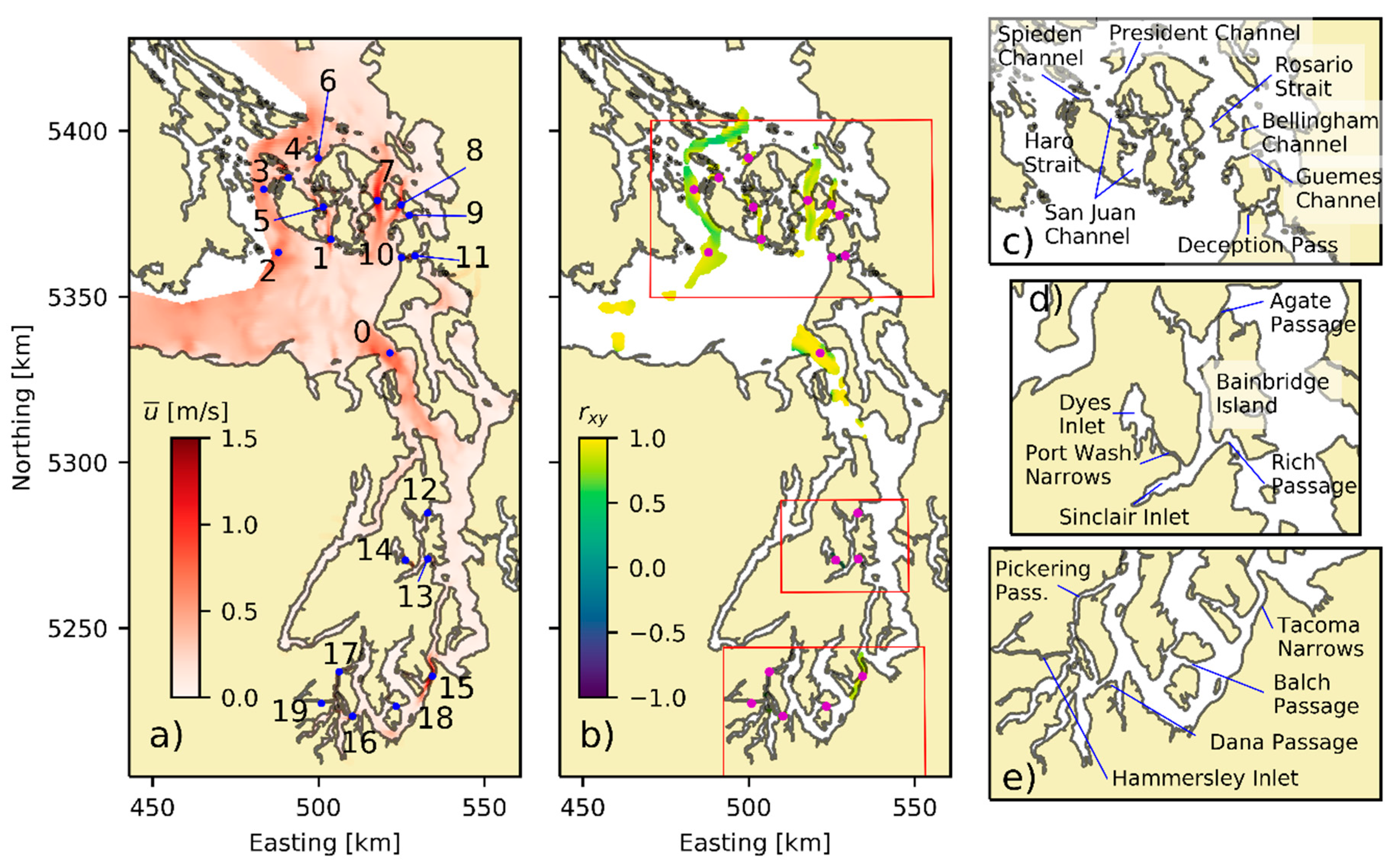
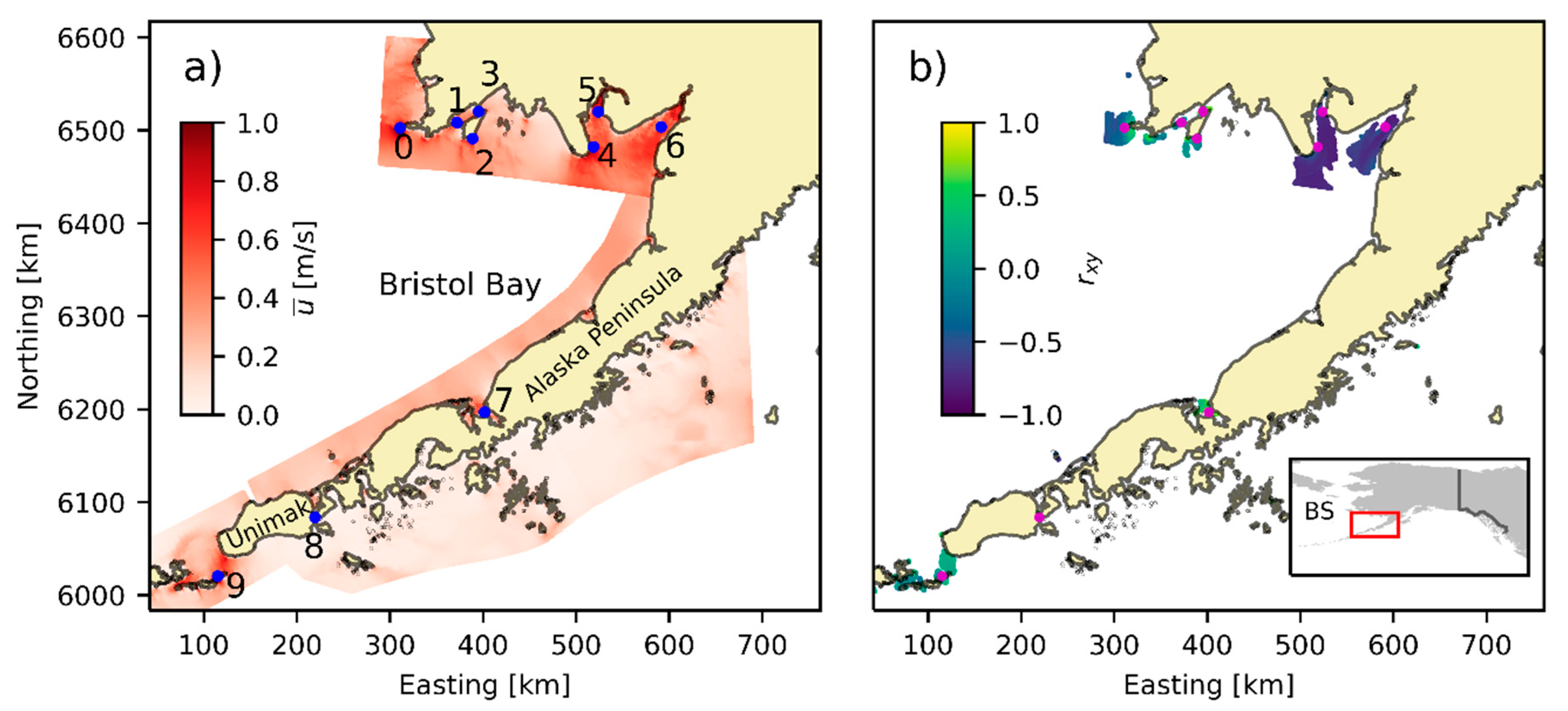
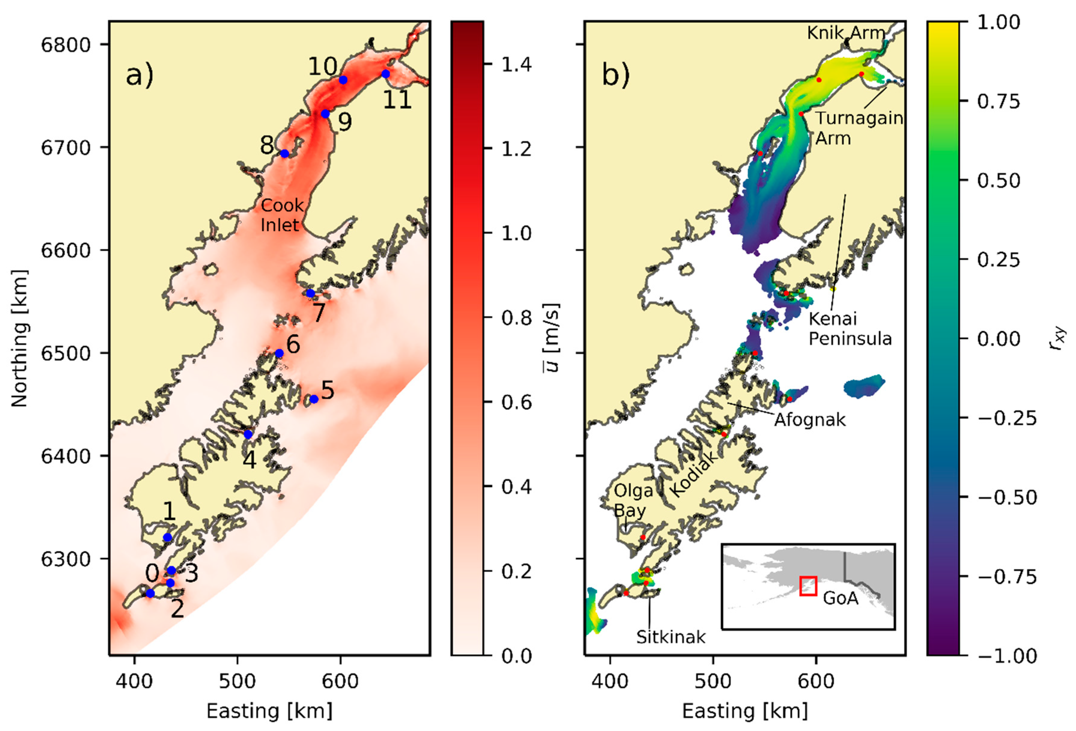
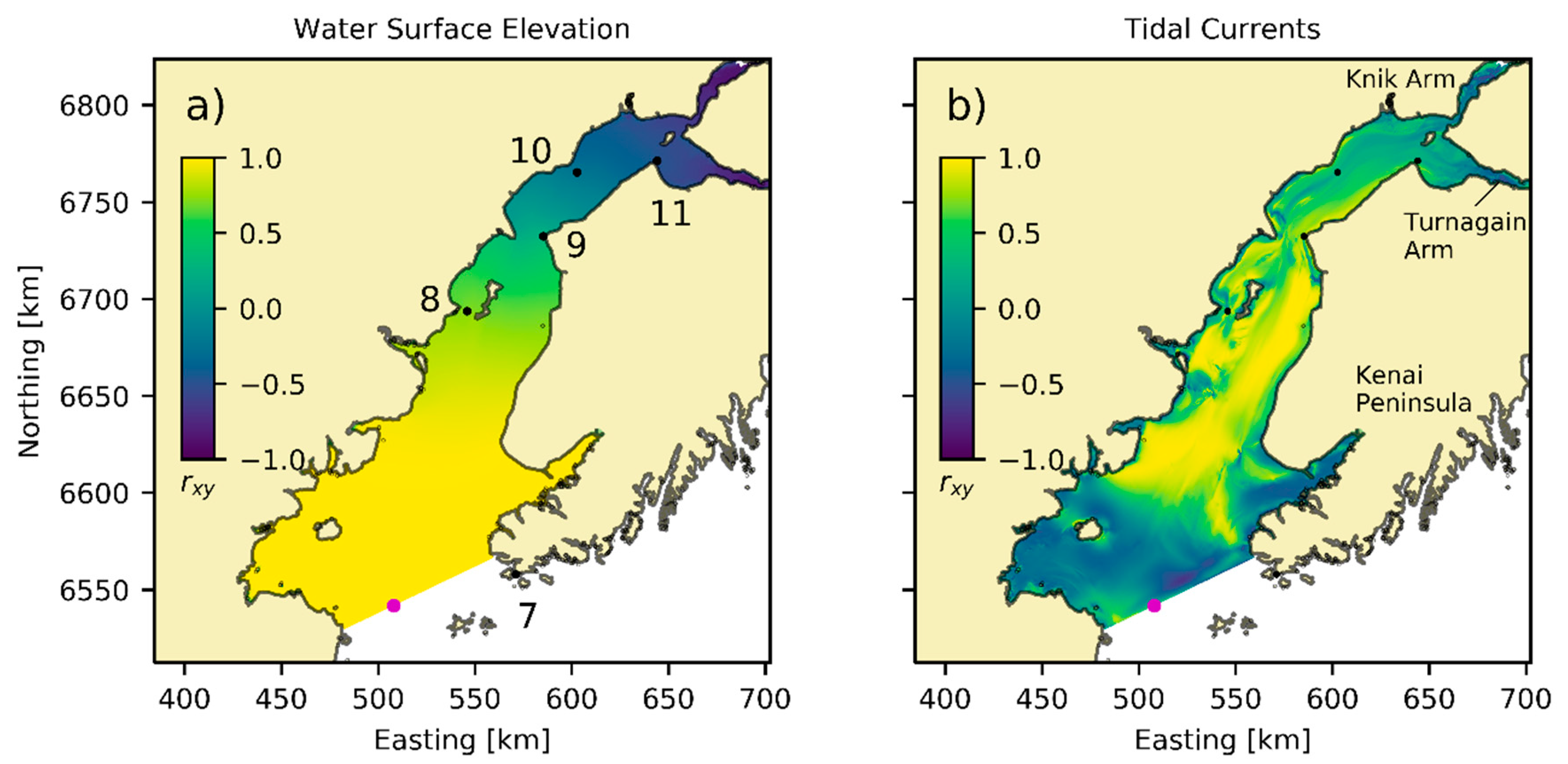
The Electrical Power Research Institute provided a first evaluation of the most energetic tidal stream sites in the United States. Sites in Alaska [4], California [5], Massachusetts [6], Maine [7], and Washington [5,7] were identified as having potential for energy extraction. Haas et al. [8] provided the first synoptic view of the tidal stream by mapping the resource in all U.S. coastal regions (except Hawaii and territories in the Pacific Ocean). The study is divided into four different regions in the U.S. Pacific Coast: Bristol Bay, Alaska; Cook Inlet and Kodiak, Alaska; Inside Passage, Alaska; and Salish Sea, Washington.

This study surveys areas known to have promise for tidal phase diversity by assessing time series of tidal velocities of representative locations in coastal areas of Alaska and Washington. This paper builds upon the work completed in [9], which analyzed the M₂ tidal constituent for the purpose of providing smoother power output through aggregation around the United States. As the most energetic tidal constituent, the M₂ represented the dominant trend in the tidal velocity patterns over time, offering a meaningful first-order analysis of the phenomenon. The work that follows introduces the full suite of tidal constituents from modeled data and verifies that modeled data to help identify locations where tidal resource aggregation (i.e., the sum of tidal power at a cluster of sites) can benefit the grid by minimizing the duration of time during which there is no power availability (slack tides) and producing smoother power profiles in aggregate.

This study will not analyze the amount of baseload or firm power that can be achieved or optimize deployment or centralized electricity dispatch decisions as that will require assumptions on the efficiency of technologies and intensity of energy extraction. Furthermore, achieving perfect baseload power is not the only way that tidal phasing can benefit the grid. Reducing the variability or fluctuation in power over time is valuable. Thus, through this inquiry, tidal phase diversity as a feasible and meaningful concept is evaluated.

To that end, Section 2 provides background information on the value of tidal energy in the United States’ grid and the natural conditions necessary to realize diverse tides within proximity. This is followed by a description of the employed mathematical methods and the data sources used in the analysis in Section 3. Results from the analysis are presented in Section 4, followed by an exploration of the practical implications for achieving smoother power profiles in practice in Section 5 and concluding remarks in Section 6.

2. Background

2.1. The Value of Tidal Energy in the United States’ Grid

Energy generation sources across the United States are transitioning from conventional energy sources that emit greenhouse gasses to cleaner, renewable energy sources. By the end of 2018, 29 states and Washington D.C. had adopted renewable portfolio standards that dictate the percentage of electricity that must be delivered from specified renewable sources by a given date [10]. These renewable portfolio standards widely vary in their goals, and many have recently updated their policies to increase their renewable supply targets from original percentages [10]. Solar and wind energy, two VERs, are dominating deployment trends, accounting for at least 95% of domestic renewable energy capacity additions [11] and 84% of global renewable energy capacity additions in 2018 [12].

As the amount of VERs increases, balancing the electric grid to ensure supply meets demand becomes increasingly complex and costly. This is particularly true for small or remote grids that are more susceptible to disruptions from variations in production and consumption. Even in a system without a significant VER penetration, operators have some foresight but limited control of electric loads. To compensate for this lack of control, traditional generating resources are designed to be predictable and controllable [13].

Notably, tidal current devices are not presently cost-effective nor have they reached a commercial state; however, given the range of grid conditions across the country and the forward-looking energy policies striving for high penetrations of renewables, it is critical to show that tidal energy resources can provide favorable characteristics from a grid perspective. Enabling decisionmakers to include and embrace these technologies as solutions and contributors in the future is necessary to reach policy goals. Identifying tidal energy’s grid-friendly traits is one step towards rethinking our conventional paradigms to deploying and valuing energy sources.

The mechanism and the rate at which renewable energy resources are adopted will differ across the country due to resource availability, favorable policy, but also the characteristics of energy capture technologies and the effects of integrating that renewable resource into the grid. As the electric grid and the generation resources feeding into it are evolving, decisionmakers have begun to modernize the way in which generation sources are incentivized and compensated, and prioritize locations where development is encouraged [14]. Innovative thinking around valuation permits grid planners, developers, and policymakers to better identify the future benefits that emerging technology could provide to a changing grid.

2.2. Tidal Conditions for Phase Diversity

Tides are caused by the gravitational interactions between the Earth, Moon, and the Sun. Because of the periodicity of the orbital motions, tides are reliable and predictable with a high level of accuracy. This predictability in the resource translates to predictability in energy production. In many parts of the world, the principal lunar semi-diurnal constituent (M₂) is the dominant tidal constituent. This tidal generating force occurs because of the gravitational interaction between the Earth and the Moon with a period of 12 h and 25 min. This period is a result of the 24-h rotation of the Earth and the rotation of the moon around the Earth.

Tides are long waves due to their long periods with respect to the depth of the ocean. Their behavior can be described by the shallow water wave equations. Long waves travel at a speed controlled by the water depth:

$$c=\frac{L}{T}=\frac{\sigma }{k}=\sqrt{gh},$$

(1)

where c is the phase velocity, L is the wave length, T is the wave period, σ (=2π/T) is the radian frequency, k (=2π/L) is the wave number, g is the gravitational acceleration, and h is the water depth.

For instance, for an M₂ tide propagating along a 200 m deep shelf the tidal phase velocity equal to $\sqrt{gh}$ = 44.3 m/s, with an associated wave length of $T\sqrt{gh}$ = 1980 km. In an inviscid environment and in the absence of interactions (e.g., friction, obstructions), tides propagate as progressive waves such that the water surface elevation (η) and the wave-induced horizontal velocity (u) are in phase with the following relationship:

$$u=\sqrt{\frac{g}{h}}\eta =\sqrt{\frac{g}{h}}\frac{H}{2}\cos \left(kx-\sigma t\right),$$

(2)

where $H$ is the tidal range.

The tidal currents are maximum under the crest and trough of the long waves. Continuing with the shelf example, regions of absolute maximum and zero horizontal velocity at the same time are 495 km apart at L/4. For that idealized tide with only an M₂ component, if two extraction sites are located at 495 km and the device can harvest in both ebb and flood tide, the aggregate theoretical power of the resources at those sites will continually be nonzero. As tides enter coastal environments, they become increasingly affected by bottom friction and by interactions with coastal features such as inlets, fjords, estuaries, etc. These interactions alter the phase relationship between η and u. This might lead to sites in proximity closer than L/4 to experience complementary tidal velocities. To account for this effect, this study considers data from multiple locations along the coasts of interest, which will be further described in Section 3.

In this study sites with high tidal current velocities are identified and the phase shifts of the tides to identify sites where large phase differences can be achieved at spatial scales shorter than L/4 are evaluated. For a topographic example of clustered but variable phasing, consider the extreme case where the ocean is connected to a large inland sea through a narrow inlet. Maximum currents will occur at the mean water level in the coastal sea. This results in a 90° phase shift between the water surface elevation and the currents and in turn a correlation of 0 between the signals (this is further discussed in Section 3.2). Additionally, tidal wave reflection and advection effects can also be present in a given system. The natural occurrence of these physical processes leads to many solutions to the wave equations where the phase of the tides is non-uniform. Due to the complex tidal circulation in natural estuaries, inlets, bays, etc. this problem cannot be fully analyzed theoretically; instead, numerical models are used in these scenarios.

Tidal currents are the quantity of interest because they are directly proportional to the instantaneous in-stream power per unit area:

$$P_d=\frac{1}{2}\rho u^3,$$

(3)

where $\rho$ is the water density. Realistically, the amount of extracted energy will be less than the theoretical resource and will depend upon energy capture efficiency and intensity of extraction. These can be included in the model by multiplying Equation (3) by the area of extraction (i.e., turbine area and number of turbines) and an efficiency factor.

3. Materials and Methods

3.1. Data Sources

Model-derived tidal currents are the primary source of data because they provide coverage at a high spatial resolution with extensive spatial coverage. Observations are used in the Salish Sea to verify the results obtained using the model-derived database; this is discussed in Appendix A.

In order to evaluate the possible complementary sites that would reduce periods of no or lower production, a consistent dataset that covers the entire area of interest is necessary. The main dataset used in this study comes from Haas, Fritz, French, Smith, and Neary [8] (H11 hereafter), which is a model-based study of tidal streams for the mainland United States, the Pacific coast of Alaska, Puerto Rico, and the U.S. Virgin Islands. Multiple overlapping models based on the Regional Ocean Modeling System (ROMS) were used to hindcast the tidal streams for a 32-day period, of which the first two days were discarded to account for spin-up effects. The models had an average spatial resolution of 350 m, for a total of 3,247,981 grid points. The models were forced using the Q₁, O₁, K₁, S₂, M₂, N₂, and M₄ constituents. The harmonic constituents and mean currents at each output point were computed using harmonic analysis on the 30-day time series. Tidal ellipses at each grid point for the main tidal constituents were available to the authors. The time series were recovered from the ellipses for each tidal constituent using the tidal ellipse toolbox for MATLAB. The final velocity time series were obtained by a adding time series from the different constituents.

Results from two refined models in the Salish Sea [15,16] (YW14 hereafter) and Cook Inlet, AK [17] (WY19 hereafter), are used to complement the results from H11. These are numerical models based on the Finite-Volume, Community Ocean Model (FVCOM) [18,19]. Similar to ROMS, FVCOM solves the Reynolds-averaged Navier–Stokes equations. However, this model implements a finite-volume approach making it suitable for coastal applications with complex shoreline geometries and topography. YW14 has a spatial resolution of ~200 m in the Puget Sound and is relaxed to 2000 m at the open boundaries outside of the Puget Sound. The model was forced with observed tides at two tidal gauges located near Neah Bay, Washington and Campbell River, British Columbia, respectively. Similarly, WY19 implements a variable resolution from 200 to 300 m inside the inlet to ~1000 m at the open boundary. This model was forced with Oregon State University’s TPXO8-atlas tidal database [20], which consists of 13 major harmonic constituents.

3.2. Methodology

With the goal of identifying sites with diverse tides that result in complementary resources, the tidal velocity time series were initially filtered for feasibility. Following similar studies estimating first-generation tidal technologies like [3], locations with modeled data with mean tidal velocities under 50 cm/s or a minimum water depth under 10 m were discarded.

Once the modeled data points below the threshold were discarded, representative locations were selected within each of the regions, one per feature (i.e., inlet, strait, headland). A cross-correlation at lag zero was calculated for the time series between each pair of locations within a region, such that

$$r_{xy}\left(0\right)=\frac{{\sum }_t\left[\left(x\left(t\right)-n_x\right)\times \left(y\left(t\right)-n_y\right)\right]}{\sqrt{{\sum }_t{\left(x\left(t\right)-n_x\right)}^2}\sqrt{{\sum }_t{\left(y\left(t\right)-n_y\right)}^2}},$$

(4)

where r_xy is the correlation coefficient, x(t) and y(t) are the tidal velocity time series, and n_x and n_y are the mean values of their respective time series. The cross-correlation indicates a measure of the time series’ movement with respect to one another. Positive correlation coefficients indicate temporal similarity between the time series patterns while negative correlation coefficients indicate dissimilarity. For the purpose of identifying complementary sites, negative correlations are ideal. The correlation coefficient does not reflect the magnitude of the sources creating a perfect offset of one another but represents the pattern of the fluctuations between the resources offsetting each other over time. Thus, a strong anticorrelation indicates decreased times of no or lower power availability when the resources are aggregated and the potential to achieve a smoother power profile. A matrix of correlation coefficients is presented for the locations within each region.

One alternate way to analyze sites for complementary phases is to compare the phases of the tidal components, e.g., [3]. This method can be implemented if looking at one tidal constituent only. Since the present study considers all the tidal constituents, this method cannot be implemented and thus the correlation method is chosen.

4. Results

4.1. Salish Sea

The Salish Sea is a large inland sea located in the Pacific Northwest Coast, bounded by the coasts of the State of Washington, USA and British Columbia, Canada. The Salish Sea is identified as a region with high potential for in-stream tidal energy extraction [21]. Previous studies have identified regions for potential tidal energy harvesting: Admiralty Inlet [16,21], Tacoma Narrows [16], Agate Pass, and Rich Passage [15]. In addition, sites in the Puget Sound with mean currents above 50 cm/s include Deception Pass, Dana Passage, Pickering Passage, and Port Washington Narrows. The flow around the San Juan Islands is also known to be energetic. To sample all channels with mean flows exceeding the 50 cm/s threshold, 20 representative points are evaluated as shown in Figure 1. In Figure 1b, cross-correlations are calculated and displayed with respect to the anchor point (0) to broadly depict diversity in the region. The cross-correlations between all sites are shown in

Table 1. Correlation table at study points around the Salish Sea from the H11 dataset.

ID	0	1	2	3	4	5	6	7	8	9
0	1	0.85	0.9	0.86	0.94	0.89	0.9	0.92	0.92	0.92
1		1	0.77	0.63	0.86	0.98	0.79	0.74	0.74	0.98
2			1	0.94	0.83	0.86	0.96	0.98	0.99	0.85
3				1	0.79	0.74	0.92	0.97	0.98	0.73
4					1	0.9	0.85	0.85	0.84	0.91
5						1	0.89	0.83	0.83	0.98
6							1	0.97	0.96	0.86
7								1	0.99	0.83
8									1	0.83
9										1
ID	10	11	12	13	14	15	16	17	18	19
0	0.21	0.18	0.9	0.82	0.05	0.89	0.78	0.64	0.73	0.63
1	0.38	0.37	0.63	0.51	−0.14	0.67	0.51	0.33	0.85	0.31
2	0.01	0.02	0.87	0.83	0.19	0.91	0.86	0.77	0.52	0.74
3	−0.12	−0.11	0.94	0.94	0.33	0.96	0.94	0.9	0.41	0.85
4	0.18	0.13	0.86	0.76	0.01	0.87	0.76	0.6	0.78	0.6
5	0.24	0.23	0.71	0.6	−0.08	0.77	0.63	0.47	0.78	0.45
6	−0.04	−0.04	0.85	0.79	0.11	0.92	0.85	0.74	0.55	0.71
7	−0.02	−0.03	0.92	0.88	0.19	0.95	0.89	0.81	0.51	0.76
8	−0.02	−0.02	0.92	0.88	0.21	0.95	0.89	0.81	0.51	0.77
9	0.34	0.32	0.73	0.62	−0.09	0.76	0.61	0.44	0.82	0.42
10	1	0.87	−0.03	−0.1	−0.12	−0.12	−0.25	−0.32	0.53	−0.31
11		1	−0.05	−0.11	−0.05	−0.13	−0.25	−0.31	0.56	−0.31
12			1	0.98	0.28	0.97	0.94	0.86	0.54	0.84
13				1	0.42	0.94	0.95	0.92	0.41	0.88
14					1	0.25	0.38	0.54	−0.16	0.48
15						1	0.97	0.89	0.5	0.86
16							1	0.97	0.34	0.95
17								1	0.17	0.97
18									1	0.19
19										1

.

Most of the points show correlations above 0, and only Deception Pass (Points 10 and 11) shows negative correlations with multiple points around the region (Table 1). As indicated by the positive correlations, there is no ideal offset generated by the tides in this region apart from combining some points with Deception Pass.

Two distinct regions are identified: San Juan Islands to the north and the Puget Sound to the south of Admiralty Inlet. In the San Juan Islands, multiple channels allow tidal flows to propagate between the Strait of Juan de Fuca and the Strait of Georgia. In the Puget Sound, most of the flow enters through Admiralty Inlet and the rest through Deception Pass [21].

In the San Juan Islands (Points 1–9), high correlations in the tides suggest minimal obstruction for propagation between the Strait of Juan de Fuca and the Strait of Georgia. Correlations are generally higher with one other and with Admiralty Inlet (Point 0), showing unfavorable conditions for aggregation to benefit the grid.

In Puget Sound (Points 0 and 12–19), the correlations decrease with distance from Admiralty Inlet (Point 0). This is a result of the tide progressing through the sound. Correlations are above 0.60 for the main channels indicating the tides flow through the main channels quickly. Maximum correlation between Admiralty Inlet and the South Sound is achieved by shifting one of the time series by one hour, indicating the time of travel of the tides between these points. This is consistent with Yang, Wang, Copping, and Geerlofs [16], who showed that the phase difference between Pickering Passage (and the southern end of the Puget Sound) is about 40 min behind Tacoma Narrows for the M₂ tide. The lowest correlation occurs with Point 14 at Port Washington Narrows. Tides entering the Puget Sound cross Point 0, then 12 and 13, before reaching Dyes Inlet through the Port Washington Narrows (Point 14). The high correlation between 0 and 12 and 13 suggests the tidal waves are slowed down near Dyes Inlet, thus increasing the lag between these points.

Deception Pass (Points 10 and 11) shows negative correlations with many of the points in the Salish Sea, including Points 3, 6–7, 12–17, and 19. These results indicate Deception Pass plays a complementary role to many other channels in the region but to a limited degree. It can become an important location for energy harvesting due to this characteristic. Although to varying degrees, having the potential to complement several locations from a timing perspective offers flexibility in planning when trying to achieve smoother power profiles through aggregation.

4.2. Alaska

Alaska contains many sites with energetic tidal flows. Due to its size, three subregions are independently analyzed: Bristol Bay, Kodiak and Cook Inlet, and Inside Passage.

4.2.1. Bristol Bay

Bristol Bay is the easternmost reach of the Bering Sea, it is known for having large tides in the upper reaches. The M₂ constituent is the most energetic one in this region and contains an amphidromic point near the north of the Bay [22]. Thus, tides follow a rotational motion around the bay, enhancing the phase diversity relative to a bay where tides propagate perpendicular to the uppermost reaches. In addition, there are several sites that exceed the velocity and depth thresholds set in the methodology. Ten representative sites were selected in this area as shown in Figure 2.

Starting from the anchor point the correlations decrease clockwise up to Point 9 at the western shore of Unimak Island, off the southwestern end of the Alaska Peninsula (

Table 2. Correlation table at study points around Bristol Bay from the H11 dataset.

ID	0	1	2	3	4	5	6	7	8	9
0	1	0.66	0.44	0.21	0.66	0.2	0.44	−0.34	−0.34	−0.35
1		1	0.83	0.54	0.92	0.18	0.59	−0.43	−0.36	−0.14
2			1	0.84	0.72	−0.2	0.2	−0.34	−0.22	0.06
3				1	0.34	−0.37	−0.13	0.02	−0.03	−0.05
4					1	0.31	0.74	−0.51	−0.46	−0.1
5						1	0.79	−0.01	−0.27	−0.31
6							1	−0.34	−0.45	−0.22
7								1	0.42	−0.12
8									1	0.51
9										1

). This trend indicates that the clockwise rotation identified for the M₂ constituent for water surface elevation is dominant when currents from the full array of constituents are considered. Many points show anticorrelations that indicate the possibility of providing smoother power profiles and reducing times of no and low production. Points 7, 8, and 9 are anticorrelated with the highest number of other sites, and those three points largely contain the strongest anticorrelations as well. Thus, not only is there flexibility in the resources that they might aggregate with for energy production, they show the highest probability of achieving smoother power profiles in the region.

4.2.2. Kodiak and Cook Inlet

Tides in the Gulf of Alaska travel from east to west [23,24] around the amphidromic point that lies between Hawaii and California. The open ocean phase difference of the M₂ tide is in the order of 20° (or 40 min) between the edge of the Kenai peninsula to the southwestern end of Kodiak Island [25]. This small phase difference is enhanced when the tide flows into Cook Inlet and the channels and banks around the islands. Twelve representative points were selected in this area as shown in Figure 3.

In the channels southwest of Kodiak Islands, Points 0, 2, and 3 are mostly in phase (

Table 3. Correlation table at study points on Kodiak and Cook Inlet from the H11 dataset.

ID	0	1	2	3	4	5	6	7	8	9	10	11
0	1	0.04	0.59	0.85	0.78	−0.23	0.22	0.44	0.29	0.42	0.91	0.88
1		1	−0.39	−0.26	−0.37	−0.31	−0.53	−0.51	0.85	0.79	0.11	−0.09
2			1	0.91	0.86	0.51	0.86	0.92	−0.3	−0.25	0.46	0.6
3				1	0.94	0.18	0.64	0.78	−0.08	0.02	0.73	0.81
4					1	0.18	0.68	0.84	−0.17	−0.08	0.75	0.85
5						1	0.77	0.59	−0.41	−0.51	−0.26	−0.09
6							1	0.94	−0.51	−0.51	0.16	0.37
7								1	−0.41	−0.39	0.39	0.58
8									1	0.97	0.38	0.13
9										1	0.5	0.26
10											1	0.94
11												1

), indicating minor tidal rotation around Sitkinak Island. Point 1 located at the Olga Narrows, a narrow strait connecting Olga Bay with the open ocean, shows anticorrelation with the neighboring points. The cross-correlations between the velocity and water surface elevation time series for Points 0 through 3 are 0.17, 0.94, −0.29, and −0.19. This shows that the flow and water surface elevation along the Olga Narrows are in phase; that is not the case for other locations around the islands. Tidal flows around Afognak Island (Points 4, 5, and 6) are also in close phase to each other and to Points 0, 2, and 3. They are in a very close phase with the entrance of Cook Inlet at Point 7. Achieving smoother power profiles within the Kodiak and Afognak system does not appear feasible based on this analysis.

Cook Inlet is known for its large tidal range and fast currents. The M₂ tide is again the most energetic component. The high tide associated with this constituent takes more than 4 h to propagate from Point 7 to Point 11 [26]. The points selected to investigate the tidal currents sample locations along the inlet. Tidal currents show a similar picture as shown by the gradients in correlations along the inlet (Figure 3b). The correlation drops monotonically from Point 8 to 11 (Table 3).

At the upstream end of Cook Inlet, Knik and Turnagain arms might extend the phase diversity of the system but are not included in this analysis because this area is not permanently submerged (Figure 4b). Overall, each of the sampled points are anticorrelated with at least one other point indicating a range of possibilities to aggregate resources at Kodiak and Cook Inlet with the strongest anticorrelations seen at Points 1, 8, and 9.

As confirmation of the correlations, data from Wang and Yang [17] (WY19) are used. The model extent and correlations are shown in Figure 4.

Table 4. Correlation table at study points in Cook Inlet based on the WY19 results.

ID	8	9	10	11
8	1	0.92	0.51	0.54
9		1	0.64	0.64
10			1	0.96
11				1

shows the correlations of the points inside the model domain. Overall the results are consistent between both models providing confidence in the results. Contrary to the analysis with the H11 dataset, these correlations were derived directly from the hourly model output. This indicates that non-tidal residuals are present, but results show the same behavior (Table 4).

The large time lags in M₂ water level propagation [17,26] can be seen from the cross-correlation analysis of the complete time series as well (Figure 4a). Correlations are taken from a point in the deepest part of the offshore boundary condition. The cross-correlation decreases monotonically upstream of the inlet as the tide propagates inward. This, however, is not reflected in the tidal currents as they fall out of phase from the water surface elevation (Figure 4b). The currents decrease monotonically upstream of Point 9. There is a small level of diversity in the upper reaches of Cook Inlet, with differences in correlations of 0.5. To enhance this diversity, points outside of the inlet must be considered.

4.2.3. Inside Passage

There are several locations in the Inside Passage of Southeast Alaska where the mean tidal velocity exceeds 50 cm/s. Some of these sites are in very shallow waters or narrow channels that, due to the model resolution, cannot be accurately modeled with a 350 m resolution. Thus, only seven points are selected for analyzing this region as shown in Figure 5.

In this region, the tide propagates northward and the phase lag for the M₂ tidal constituent, the most energetic, is around 25° [22]. However, there is a significant phase difference when the tidal currents are evaluated. Multiple sites show negative correlations as shown in

Table 5. Correlation table at study points in the Inside Passage, Alaska.

ID	0	1	2	3	4	5	6	7
0	1	0.71	0.71	−0.39	0.69	0.18	0.68	−0.4
1		1	0.89	−0.61	0.22	−0.23	0.14	−0.52
2			1	−0.4	0.33	−0.07	0.26	−0.38
3				1	0.15	0.63	0.16	0.9
4					1	0.74	0.94	0.1
5						1	0.76	0.62
6							1	0.11
7								1

. Tidal currents north and south of Chichagof Island are out of phase where Point 3 shows correlations between −0.61 and −0.4 with points in the north. Overall, the potential to aggregate resources to reduce periods of no or low power production and achieve smoother power profiles in the region exists at Points 3, 5, and 7. Point 3 is also anticorrelated with Points 0 and 1, which are all around Chichagof Island.

Local effects play a dominant role since the water surface elevation between Points 1 and 3 are highly correlated at 0.95 (not shown). Further, cross-correlation analysis of water surface elevation is at least 0.89 for all points in the region. Similarly, Point 7 is not correlated with the northern tidal flows. This case is opposite to Cook Inlet where there is more phase diversity in the water surface elevation than in the tidal currents.

5. Discussion

Of the evaluated regions, pairs of points in Cook Inlet and Bristol Bay indicate the highest probability of reducing times of no power availability and smoother power output through aggregation. The extent to which the resource can be exploited to realize these benefits depends on development decisions, device controls, project economics, infrastructure, and institutional limitations. It is important to note that the analysis considers the correlation of the velocity time series and indicates patterns between the resources, not actual power produced from the specific extraction of the resources. Therefore, even if a strong anticorrelation exists between the resources at two locations, the magnitude of those resources is not explicitly considered. That is to say that the general pattern and fluctuation of the resources complement one another at the evaluated time scale, but one resource could have a much higher average velocity at one location compared to the other and would necessitate development decisions that capitalize on the behaviors that enable smoother power profiles in aggregate.

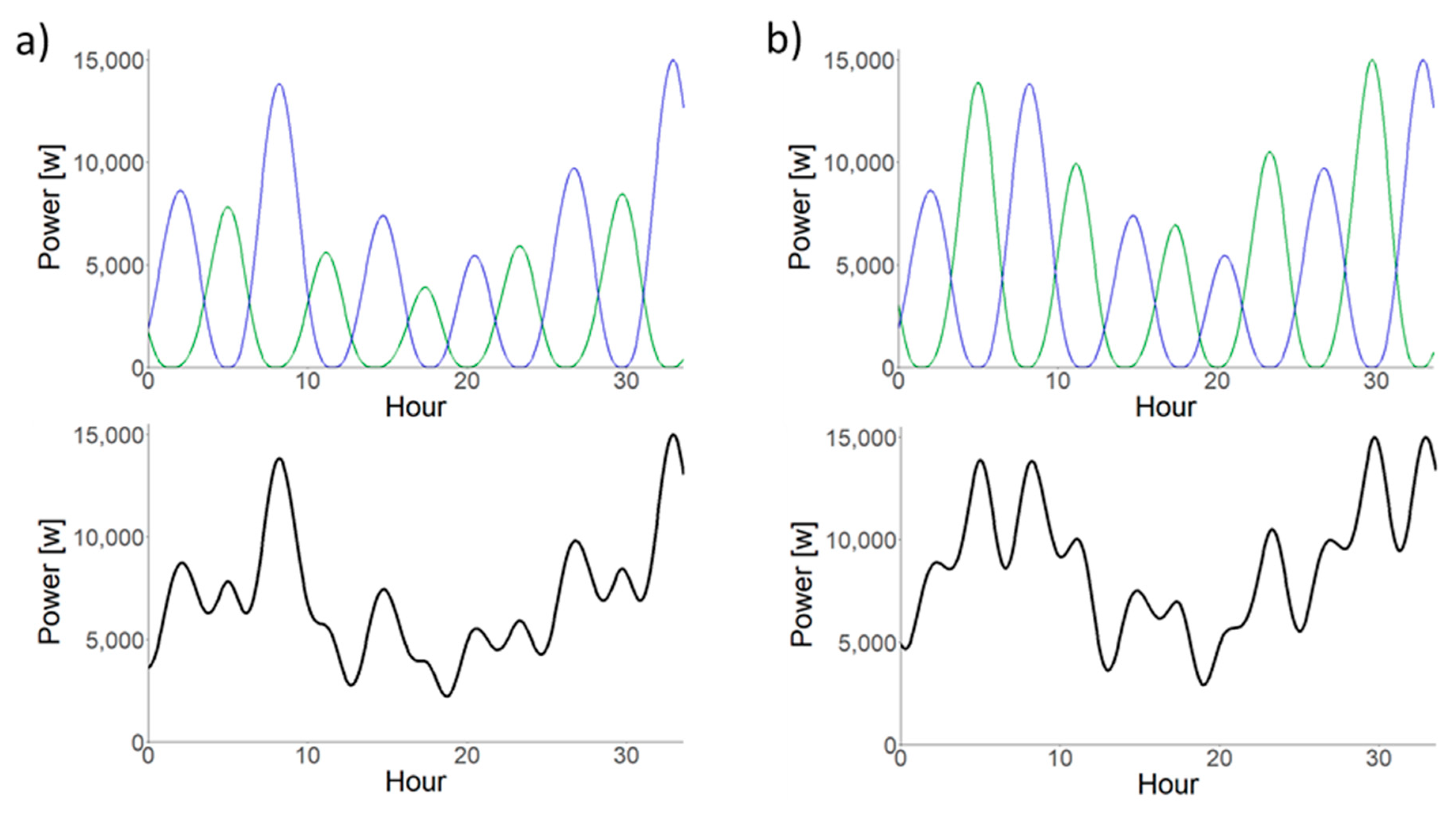
Results with strong anticorrelations indicate a decrease in times of no or low power availability and thus, the possibility of producing smoother power profiles in aggregate. For example, Points 6 and 8 at Cook Inlet have an anticorrelation of −0.51. Translating the velocity at those locations into theoretical power, Figure 6a is generated. The power time series of those individual points show five and six periods of no power availability during the displayed time, but in comparison, the aggregate power from the time series does not have any periods lower than 160 watts. Thus, as indicated by the 160-watt minimum, the aggregate power time series has a nonzero power minimum for the duration of the evaluated time period.

The intensity at which the resources are extracted is also important, as that contributes to the potential for smoother power output. By scaling the theoretical power time series to have the same maximum power value (i.e., mimicking disproportionate development to generate similar amounts of power by increasing the capture area), Figure 6b is generated. In comparison to Figure 6a, the aggregate power does not drop below 200, the maximum aggregate power only increases trivially, and the continual steepness of the ramping has decreased. With fewer dips in available power, there is the opportunity to generate smoother power by limiting the upper capacity of production. It is important to note that these estimations do not consider the efficiency of the devices cut-in or cut-out speeds associated with turbines, but rather focus on the theoretical power. Further, the effects of tidal asymmetry due to the superposition of various tidal constituents can be seen in the example aggregated power (Figure 6) where consecutive cycles can have variations of more than 100% in peak power. When multiple sites are considered in order to achieve continuous power, the aggregated effect of this asymmetry can be large and must be analyzed in detail at the time of selecting the technology and intensity of extraction. Siting tidal energy converters in ebb and flood dominated parts of a strait has been shown to reduce the variability in peak power production [27,28]. Moreover, the rectilinear misalignments between the dominant flood and ebb directions will have additional impacts on actual power production. Thus, all these factors should be carefully considered in future, finer-scale case studies.

There are a number of ways in which smoother power output can be achieved and optimized in practice. They are dependent upon site-specific needs, including those dictated by the grid, and those needs vary by location. Aggregating diverse tides generates an optimization question of how and the extent to which the resources should be harnessed. Part of this optimization is not simply evaluating the hour by hour comparison between the resources but also analyzing the aggregate power over the spring–neap cycle. Weaker resources at one location might need to be extracted at a higher intensity than complementary resources at a location with stronger current velocities to reduce periods of no and low production. To produce smoother power from complementary resources, limiting turbine capacity is an option to cap the maximum production from machines and decrease the range in power output, as also noted in [1]. There are economic implications of limiting power for the purpose of providing smoother power such that decreasing turbine capacity can improve a project’s capacity factor and increase project economics [1], but the amount of energy produced over time will be reduced. However, even if the tidal resources are present, institutional mechanisms must be in place for the grid to realize the complementarity benefits and to produce favorable economic results.

In the analysis, reasonable spatial boundaries to “cluster” tidal profiles were applied. Conceptually, each individual tidal project or turbine would not be directly or operationally connected to one another in the water; rather, the smoother net profile or reduction in periods of no or low production is achieved by grid-side aggregation. Aggregator is a term commonly applied to a third party or activity that compiles distributed energy resources into one virtual power plant in order to have a single point of economic transaction. While aggregation is sometimes useful for small generators that are not large enough to enter into complex markets, for tidal resources, a greater value may be achieved through aggregating profiles into a predictable block of energy.

There are limits to aggregation, however. This is principally linked to whether the facilities are located in the same electricity management footprint, rather than whether they are physically nearby. In this electricity footprint, one operator balances electric load and generation in real-time. Electricity boundaries are not necessarily related to political or geographical boundaries, and in some cases, the footprint can be very large. Almost all of the state of California is managed by one operator, the California Independent System Operator (CAISO), which offers options for distributed energy resource aggregators [29].

Therefore, in order to capture the grid benefits of tidal phase diversity for a reduction in periods of no or low production or a smoother power profile, facilities do not need to be close physically, but they need to be close electrically. Once tidal phase diversity is identified, the next steps are to establish points of interconnection and evaluate the ability to aggregate and reach a single off-taker, whether a load-serving utility or a market. In environments with many small isolated electrical systems—e.g., as is common in Alaska—aggregation may not be feasible. Similarly, even perfectly phased tidal regimes, if spread over a very large geographic range, would likely be economically impractical if not under a single system operator. Understanding these requirements in locations where aggregating tidal resources may provide grid benefits is key to moving from theory to reality.

6. Conclusions

This paper shows there is limited potential in areas of Alaska and Washington for tidal phase diversity to reduce periods of no or low power availability and generate smoother power profiles through aggregation. Locations around Kodiak Island and Cook Inlet show the greatest potential out of the evaluated regions with each of the sampled locations there anticorrelated with at least one other location and several sites showed strong anticorrelations. Locations at Bristol Bay and Inside Passage also present the opportunity to exploit resources for this purpose, but to a more limited degree and over a larger geographic footprint. Finally, locations around Washington are significantly more restricted in their feasibility based on the available resources.

Data from [16] were verified with measurements and other modeled data in the Salish Sea [15,16] and also compared to modeled data from [17] in Alaska. Practical considerations for the phenomenon to be realized in practice were outlined, and it was established that while the concept of tidal phase diversity has limited potential to feasibly benefit the grid around Washington and Alaska, site-specific analyses would be required to determine the practicality of developing the resources in any identified locations for this purpose.

References

1. Clarke, J.A.; Connor, G.; Grant, A.D.; Johnstone, C.M. Regulating the output characteristics of tidal current power stations to facilitate better base load matching over the lunar cycle. Renew. Energy 2005, 31, 173–180. [Google Scholar] [CrossRef]
2. Giorgi, S.; Ringwood, J.V. Can Tidal Current Energy Provide Base Load? Energies 2013, 6, 2840–2858. [Google Scholar] [CrossRef] [Green Version]
3. Neill, S.P.; Hashemi, M.R.; Lewis, M.J. Tidal energy leasing and tidal phasing. Renew. Energy 2016, 85, 580–587. [Google Scholar] [CrossRef] [Green Version]
4. Polagye, B.; Bedard, R. Tidal in-Stream Energy Resource Assessment for Southeast Alaska; Electric Power Research Institute: Palo Alto, CA, USA, 2006. [Google Scholar]
5. Bedard, R.; Previsic, M.; Siddiqui, O.; Hagerman, G.; Robinson, M. North American Tidal in Stream Energy Conversion Feasibility Demonstration Project; EPRI TP-04-NA; Electric Power Research Institute: Palo Alto, CA, USA, 2006. [Google Scholar]
6. Hagerman, G.; Bedard, R. Massachusetts Tidal in-Stream Energy Conversion (TISEC): Survey and Characterization of Potential Project Sites; Electrical Power Research Institute: Palo Alto, CA, USA, 2006. [Google Scholar]
7. Hagerman, G.; Bedard, R. Maine Tidal in-Stream Energy Conversion (TISEC): Survey and Characterization of Potential Project Sites; Electric Power Research Institute: Palo Alto, CA, USA, 2006. [Google Scholar]
8. Haas, K.A.; Fritz, H.M.; French, S.P.; Smith, B.T.; Neary, V. Assessment of Energy Production Potential from Tidal Streams in the United States; Georgia Tech Research Corporation: Atlanta, GA, USA, 2011. [Google Scholar]
9. Preziuso, D.; García Medina, G.; O’Neil, R.; Yang, Z. Evaluating the tidal energy resource for smooth power output and grid integration in the United States. In Proceedings of the 2019 IEEE OCEANS Conference Proceedings, Seattle, WA, USA, 27–31 October 2019. [Google Scholar]
10. Barbose, G. U.S. Renewables Portfolio Standards: 2019 Annual Status Update; Lawrence Berkeley National Laboratory: Berkeley, CA, USA, 2019.
11. U.S. Energy Information Administration. Electric Power Annual 2018; U.S. Energy Information Administration: Washington, DC, USA, 2019.
12. International Renewable Energy Agency. Renewable Capacity Highlights; International Renewable Energy Agency: Abu Dhabi, United Arab Emirates, 2019. [Google Scholar]
13. Kirby, B.; Ela, E.; Milligan, M. Analyzing the Impact of Variable Energy Resources on Power System Reserves. In Renewable Energy Integration: Practical Management of Variability, Uncertainty and Flexibility in Power Grids; Academic Press: Cambridge, MA, USA, 2014; pp. 83–99. [Google Scholar]
14. State of New York Public Service Commission. In the Matter of the Value of Distributed Energy Resources. In 15-E-0751; State of New York Public Service Commission: Albany, NY, USA, 2019. [Google Scholar]
15. Wang, T.P.; Yang, Z.Q. A modeling study of tidal energy extraction and the associated impact on tidal circulation in a multi-inlet bay system of Puget Sound. Renew. Energy 2017, 114, 204–214. [Google Scholar] [CrossRef]
16. Yang, Z.Q.; Wang, T.P.; Copping, A.; Geerlofs, S. Modeling of in-stream tidal energy development and its potential effects in Tacoma Narrows, Washington, USA. Ocean Coast. Manag. 2014, 99, 52–62. [Google Scholar] [CrossRef]
17. Wang, T.; Yang, Z. A Tidal Hydrodynamic Model for Cook Inlet, Alaska, to Support Tidal Energy Resource Characterization. J. Mar. Sci. Eng. under review.
18. Chen, C.S.; Huang, H.S.; Beardsley, R.C.; Liu, H.D.; Xu, Q.C.; Cowles, G. A finite volume numerical approach for coastal ocean circulation studies: Comparisons with finite difference models. J. Geophys. Res. Oceans 2007, 112. [Google Scholar] [CrossRef]
19. Chen, C.S.; Liu, H.D.; Beardsley, R.C. An unstructured grid, finite-volume, three-dimensional, primitive equations ocean model: Application to coastal ocean and estuaries. J. Atmos. Ocean. Technol. 2003, 20, 159–186. [Google Scholar] [CrossRef]
20. Egbert, G.D.; Erofeeva, S.Y. Efficient inverse Modeling of barotropic ocean tides. J. Atmos. Ocean. Technol. 2002, 19, 183–204. [Google Scholar] [CrossRef] [Green Version]
21. Polagye, B.; Kawase, M.; Malte, P. In-stream tidal energy potential of Puget Sound, Washington. Proc. Inst. Mech. Eng. Part A J. Power Energy 2009, 223, 571–587. [Google Scholar] [CrossRef]
22. Shi, L.; Wang, J.; Myers, E.; Huang, L. Development and Use of Tide Models in Alaska Supporting VDatum and Hydrographic Surveying. J. Mar. Sci. Eng. 2014, 2, 171–193. [Google Scholar] [CrossRef]
23. Irish, J.; Munk, W.; Snodgrass, F. M 2 amphidrome in the northeast pacific. Geophys. Fluid Dyn. 1971, 2, 355–360. [Google Scholar] [CrossRef]
24. Luther, D.S.; Wunsch, C. Tidal Charts of Central Pacific Ocean. J. Phys. Oceanogr. 1975, 5, 222–230. [Google Scholar] [CrossRef] [Green Version]
25. Isaji, T.; Spaulding, M.L. A Numerical Model of the M2 and K1 Tide in the Northwestern Gulf of Alaska. J. Phys. Oceanogr. 1987, 17, 698–704. [Google Scholar] [CrossRef] [Green Version]
26. Kowalik, Z.; Proshutinsky, A. Tsunami–tide interactions: A Cook Inlet case study. Cont. Shelf Res. 2010, 30, 633–642. [Google Scholar] [CrossRef]
27. Guillou, N.; Chapalain, G. Tidal Turbines’ Layout in a Stream with Asymmetry and Misalignment. Energies 2017, 10, 1892. [Google Scholar] [CrossRef] [Green Version]
28. Neill, S.P.; Hashemi, M.R.; Lewis, M.J. The role of tidal asymmetry in characterizing the tidal energy resource of Orkney. Renew. Energy 2014, 68, 337–350. [Google Scholar] [CrossRef]
29. California Independent System Operator Corporation: Fifth Replacement FERC Electric Tariff; California Independent System Operator Corporation: Folsom, CA, USA, 2019; pp. 109–111.
Figure 1. Salish Sea study area. (a) Mean tidal current speed and (b) cross-correlation at points with a mean velocity above 50 cm/s with respect to the anchor point (0). Representative points for the correlation analysis are identified. Points identified are (0) Admiralty Inlet, (1) San Juan Channel South, (2) Haro Strait South, (3) Haro Strait North, (4) Spieden Channel, (5) San Juan Channel, (6) President Channel, (7) Rosario Strait, (8) Bellingham Channel, (9) Guemes Channel, (10) Deception Pass West, (11) Deception Pass East, (12) Agate Passage, (13) Rich Passage, (14) Port Washington Narrows, (15) Tacoma Narrows, (16) Dana Passage, (17) Pickering Passage, (18) Balch Passage, and (19) Hammersley Inlet. (ce) Close-ups of the study area. Location map is shown in Figure A1.
Jmse 08 00246 g001
Figure 2. Bristol Bay study area. (a) Mean tidal current speed and (b) cross-correlation at points with mean velocity above 50 cm/s and deeper than 10 m with respect to the anchor point (0). Representative points for the correlation analysis are identified in both figures. BS stands for Bearing Sea in (b).
Jmse 08 00246 g002
Figure 3. Cook Inlet and Kodiak study area. (a) Mean tidal current speed and (b) cross-correlation at points with mean velocity above 50 cm/s and deeper than 10 m with respect to the anchor point (0). Representative points for the correlation analysis are identified on both panels. GoA stands for Gulf of Alaska.
Jmse 08 00246 g003
Figure 4. Cross-correlations for water surface elevation (a) and depth-averaged tidal currents (b) based on WY19 with respect to the open boundary point in magenta.
Jmse 08 00246 g004
Figure 5. Inside Passage, Alaska study area. (a) Mean tidal current speed and (b) cross-correlation at points with mean velocity above 50 cm/s and deeper than 10 m with respect to the anchor point (0). Representative points for the correlation analysis are identified on both panels.
Jmse 08 00246 g005
Figure 6. Power (a) and scaled power (b) at Cook Inlet Point 6 (green) and Point 8 (blue) above the aggregate power density of the two locations.
Jmse 08 00246 g006