1. Introduction
Today, exploitation activities are mainly done in deep waters far from the coastal area. Furthermore, for easier maintenance and transportation, drilling rigs usually float on water. However, cargo ships cannot be anchored under such conditions and need a complex DP technique to maintain their stationary position and direction relative to a reference point on the sea surface. The required criteria for performing a given task, as well as the surrounding conditions and expectations of behaviors for various natural phenomena together have an impact on designing DP systems and their forms of operations.
The design of such systems largely depends on their purpose. Therefore, it is necessary to identify the environmental conditions in which the ship will navigate and perform operations. Namely, ships are exposed to environmental forces and moments such as wind, waves, and current, which produce motion disturbances. To enhance the accuracy of such systems, proper controller design is required to process measured signals from various sensor devices and calculate the ship dynamic properties. Error minimization could be done with a fine estimation of wave conditions. This is significant because of reducing the possibility of critical situations, both for passengers and cargo on board, as well as providing a sense of stability and safety. In addition to moored buoy, satellite, and radar measurements, which have been in use for many years, a DWS estimation based on measured ship motions has proved to be much easier in terms of maintenance [
1,
2,
3].
In addition to the control algorithm, it is important to determine the proper filtering algorithm (in terms of reconstruction and subsequent estimation) for processing noisy signal measurements. An efficient approach for noise removal is based on time-frequency (TF) distribution methods. Additionally, adaptive, data-driven filtering methods in the TF domain may be used to enhance the accuracy of positioning systems and ship mathematical models. Fundamental methods of signal processing procedures, such as the Fourier transform, assume that the frequency features do not change with time. However, when the spectral characteristics of the analyzed signal are time varying, this approach gives a mean spectral representation and results in low-frequency resolution if estimates are obtained using short time windows or filter banks. Consequently, most of these techniques are inefficient for non-stationary signals, which most often appear in real life. This led to the creation of new concepts for representing signals together in the time and frequency domain [
4,
5,
6].
Individually, sensors cannot provide enough accurate and reliable information on measured data. Therefore, measurement systems are observed simultaneously, forming an integrated navigation system. Advanced estimation techniques use multiple various sensors together [
7]. Missing information from one of the sensors is provided by measurements of other sensors. By comparing the theoretical and measured conditions, it is necessary to reduce the error variation and thus contribute to the accuracy of the system. The use of KF methods has proven to be a very reliable technique in such situations, providing optimal state estimates, both for linear and nonlinear systems.
Techniques to improve the accuracy and reliability of the ship’s positioning system have been developed over the years. This paper provides a detailed overview of the methods used in control and filtration algorithms and is structured as follows. Firstly, in
Section 2, ship shifts, speeds, and accelerations are considered in terms of their changes during various sea states, as well as the impacts of external forces. The six degrees of ship’s motion are divided into three rotational degrees of motion and three linear motion degrees with associated transverse, longitudinal, and vertical accelerations. Next,
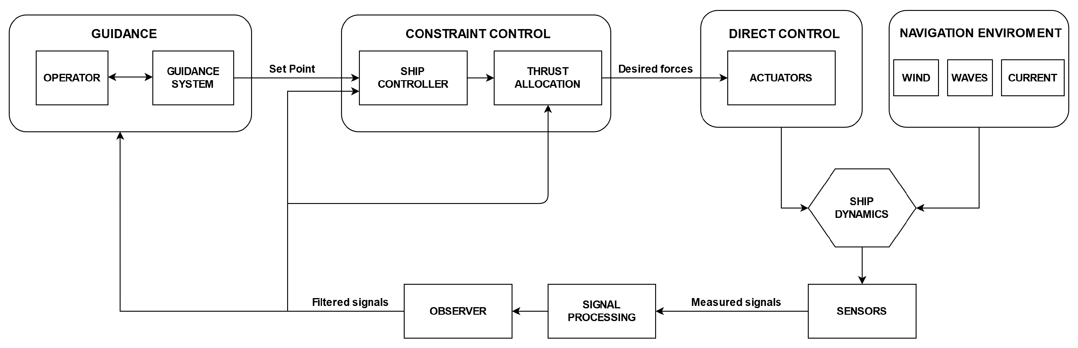
Section 3 provides a schematic diagram of the dynamic ship positioning system in a closed feedback loop. The mechanical and electrical aspects of the individual system blocks, which together perform the tasks of filtration and signal processing, and finally, the control of the actuators, are described. Related to that,
Section 4 gives an overview of DWS estimation methods, as well as an introduction to various signal filtering and reconstruction methods. The section describes new estimation approaches based on ship motion processing. Descriptions of two formulations of estimation methods in terms of the cost function optimization are given.
Section 4 gives an insight into various past and current trends in the TF signal analysis domain. An overview of the standard and adaptive methods is reviewed and divided into non-parameterized, adaptive, and parameterized TF analysis methods. The section also gives a parallel comparison of the TF distributions of measured signals. Real data ship responses are shown for various ship motions, as well as angular velocity and accelerations. The advantages and disadvantages of individual methods are outlined, and it is emphasized that more different methods should be used to achieve better results. Finally,
Section 5 deals with advanced filtering techniques that use the KF, based on a series of measurements in time, as well as statistical information of noise and interference. This filtering method has experienced widespread use in navigation systems for estimating unknown variables that cannot be measured directly, as well as for overcoming white and colored noise from the estimated states using measurements from multiple sensors of different accuracy [
8,
9,
10].
2. Ship Motions and Accelerations
When a ship sways due to the exciting forces and moments of the waves, its swing produces hydrostatic and hydrodynamic forces. Hydrostatic forces return the body to its initial state and are referred to as return forces. Hydrodynamic forces dampen the resulting oscillation motion. Every ship is subjected to six degrees of motion due to external forces. These forces produce accelerations defined as the rate of change of velocity. Under its propulsion, the ship accelerates or decelerates, due to the influence of stern seas or head seas. More importantly, though, are the accelerations caused by external forces such as the wind, sea, and currents [
11]. To explain the ship motions as precisely as possible, we will consider the motion’s impact on the cargo carried by the ship.
Under the influence of external forces, the ship is subjected to three rotational degrees of motion. These motions are rolling, pitching, and yawing, termed as “rotational movements” since every ship partially turns around its front and back longitudinal axis when rolling, around its transverse axis when pitching, and around its vertical axis when yawing. Furthermore, there are three linear degrees of motion. These are surging, swaying, and heaving introduced as “linear” since the ship surges along its front and back longitudinal axis, sways to some point along its transverse axis, and heaves up and down along its vertical axis [
12]. The described six degrees of motion are illustrated in
Figure 1.
When the ship’s cargo encounters the crushing force, the ship lashing system undergoes trials. The ship cargo, which constantly lifts and falls due to heaving, would be lifted and dropped, thereby impacting compression and tensile forces to lashing components. Similarly, when the ship starts moving between two waves, the lashing rods experience forces in opposition to those experienced when the ship moves up a wave profile. Likewise, when ship pitches, the lashing rods tend to be alternately stretched and compressed.
The six degrees of motion combine in different ways to produce the resulting accelerations. First are the transverse accelerations that act across a ship’s hull in the transverse direction. Next are the longitudinal accelerations that move along a ship’s hull in the front and back direction. The last ones are vertical accelerations that act up and down perpendicular to a ship’s hull. Vertical forces are those forces acting normally on the hull, while transverse forces are those acting over it. The acceleration rates are usually estimated for a specific ship before its first operation at sea. Transverse and vertical accelerations are estimated from the shape of the ship surface, its maximum width and length, and the relative positions of the centers of gravity and buoyancy, as recorded from model testing. However, the actual behavior of a ship at sea is not fully known during the ship’s design stage, and acceleration values can only be estimated. Rolling, pitching, and heaving are the most common of the six degrees of motion and generate the largest accelerations (pitching and rolling generate acceleration forces that increase with distance from the roll or pitch axis).
When the ship moves through the water with constant speed, the cargo is carried in the same line of motion and with the same speed as a ship. If no external forces act on the ship, then no forces will be transferred to the cargo and associated components. On the other hand, if the ship goes in the direction of some point at the sea surface (by rudder movements or under the influence of heavy seas), there would be an automatic speed reduction producing decelerations that, in turn, would produce certain forces. These forces will be transferred to the cargo and lashing components. When the ship is forced upwards, it eventually comes to rest on the crest of a wave, and when it moves down, it eventually comes to rest in the trough of a wave. During this cycle, the water plane areas are changing rapidly and affect the ship’s buoyancy. Vertical acceleration forces are mostly produced during heaving, but also, to a lesser extent, by pitching and rolling. Longitudinal acceleration forces are mainly caused by pitching and, to a lesser extent, surging and yawing. Transverse acceleration forces represent the most important factor when creating the lashing system for a particular sea plan and season of the year. These accelerations are mainly caused by rolling and, to a lesser extent, by a combination of yaw and sway motions. Roll angles are related to the extent of the transverse accelerations produced. If these values fall outside of the ship parameters, for a particular sea route in heavy weather, containers may befall overboard from high stowage locations. High roll angles often occur in following seas. Whilst following seas assist the speed of the ship, longitudinal and vertical accelerations will be generated [
13].
External (environmental) forces of induced waves, winds, and sea currents have an oscillatory (stochastic) nature. These forces are introduced as disruptions, which enter the system and have an impact on the ship motions. Conceptually, these forces can be separated into second-order low-frequency forces and first-order high-frequency forces. Therefore, ship motions are often referred to in the context of slowly varying character low-frequency motions and high-frequency motions where the total ship motions are then equal to the sum of the low-frequency and high-frequency components.
High-frequency (wave-frequency) disturbances are produced by high-frequency, wave pressure-induced forces, which have a frequency content at the sum of the wave frequencies and have a fast oscillating character. These forces are not considered in the control algorithm because of too high-frequency content, but may affect the vibrations in the ship hull. On the other hand, forces with low-frequency content can cause the ship to move horizontally, so they are taken into account as feedback signals in DP systems. In addition, the induced forces of wind and sea currents are taken into account. Only mean components are considered for wind forces until the components caused by the gusts are not measured by the ship’s responses. The forces of the sea currents have low-frequency content and may also be significant to consider in DP systems [
14,
15].
4. Estimation of DWS
Hydrodynamic wave-induced ship motions can affect all ship systems, as well as the ship’s crew. By predicting the forces and moments acting on the hull, it is possible to predict the movements of the ship in particular conditions, even in real time. Improving accuracy and optimizing the DP system performance is done with a fine estimation of DWS, which further improves the efficiency, safety, and stability of navigation, reflecting on the ship’s system, as well as the crew. With available measurements, the fundamental problem is to get information about DWS data to update the system continuously.
Conventional techniques utilize moored buoys for measurements of the wave’s height and direction, as well as satellite and radar devices. Moored buoys are reliable and are the primary means of collecting wave data. This issue of such devices exists because of the performance and maintenance complexity, low-resolution properties, as well as their price and high sensitivity to system errors and weather damage [
1,
2,
3,
11,
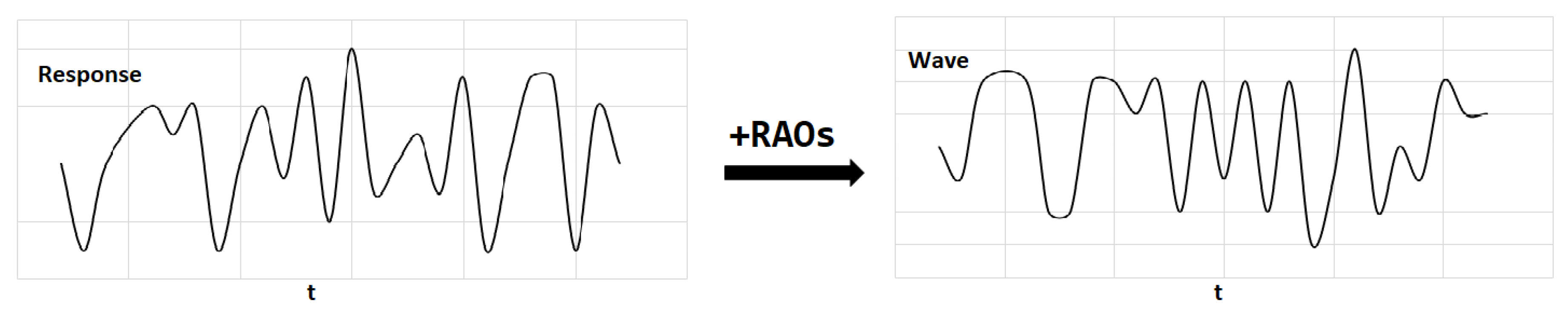
24]. Due to the disadvantages of conventional devices, DWS estimation methods have been extended to process measurements of ship motions (especially the roll, pitch, and heave motions) and their couplings. Such procedures can be done on-board and do not require complex devices. Furthermore, measurements are much easier to implement and provide accurate and reliable outcomes. According to the wave buoy analogy, a ship can also be observed as a unique buoy (sensor). Therefore, the ship can represent a hydrodynamic response to the waves and provide information on the state of the sea, using all actual sensors in real time. The similarity with the process of moored buoys is in the assumption of a linear relationship between waves and associated motions. This approach is still under development and could prove to be a very good alternative to conventional estimation methods.
Figure 4 represents a block diagram of the principal idea of the DWS estimation process with the use of measured motion responses. One can see that the purpose of this technique is to perform an estimation of input data based on measured output data. After signal processing, the measured and calculated response spectra are compared with each other, and the measurement error can be minimized to give a more precise and reliable estimation. From the 1970s to the present, many studies have been conducted, and many methodologies have been developed concerning the estimation of DWS using motion responses. Research on the estimation procedures up to 2010 was mainly based on the wave buoy analogy with formulations in the frequency domain. With the improvement of computing resources, nonlinear optimization methods [
2] were further developed, as well as formulations in the time domain [
25]. A full review of common methods and formulations was given in the work of Nielsen et al. (2017) [
1].
Estimation methods depend on the previous knowledge of the ship performance in particular wave conditions. These characteristics are specified using complex transfer functions (a complex number that contains the amplitude and phase information) or so-called response amplitude operators (RAO), also indicated in the block diagram in
Figure 4. Assuming linearity, the mathematical relationship between the measured response spectra and the DWS in the frequency domain is theoretically given by the following equation [
1,
24,
26,
27]:
where the theoretical relationship of the ith and jth components of the measured response spectrum
and the directional wave spectrum
is given by the complex transfer functions
and
(complex conjugate). Herewith, the DWS and measured response spectrum are given for encountered frequencies
, wave frequencies measured from the ship’s point of view. A graphical representation of the DWS estimation for the formulations in the frequency domain is given in
Figure 5.
RAO transfer functions and DWS are given for different wave directions relative to some fixed direction
. The representation example of RAO amplitudes, relative to the wave frequency and wave direction, are given in
Figure 6 for three ship responses, roll, pitch, and heave. Amplitudes are shown for a ship speed of 16.19 knots and various headings. To improve the view, extra points are obtained by the interpolation process. The example data were derived from the data of a 28,000 DWT bulk carrier, 160 m in length, which sailed in the southern seas.
Considering the ship course (which we can denote by
) as a fixed direction, the wave direction will be equal to the heading of the ship relative to the waves (the so-called encountered angle, which can be denoted as
). This equality follows from the following equation [
11,
27,
28]:
This encounter angle corresponds to head waves if
, and the relation for all sea states is shown in
Figure 7, with
given in degrees.
The mathematical model of the DP system is formulated to compare the measured (left equivalent in Equation (
1) and theoretical (calculated right equivalent in Equation (
1)) spectral responses, also shown in the block diagram in
Figure 4. Typically, three independent motions are simultaneously considered to uniquely determine the wave direction reliably. These are the roll, pitch, and heave motions that are least caused by the thrusters [
24]. A direct comparison of the theoretical relation can be obtained by defining governing equations of the estimation problem with a set of measured spectral responses. This problem can be solved by the minimization process defined with [
1]:
where
is a vector function of DWS and
b contains information about the measured response spectrum. The
A matrix is designed based on the RAO transfer functions.
The above theoretical Equation (
1) assumes zero-forward speed, but since the wave spectrum is favorably estimated in the domain of true wave frequencies (
), it is necessary to consider this forward speed, which further contributes to the complexity of the system [
24]. Namely, under the condition of following seas (direction shown in
Figure 7), at specific encounter frequencies
, three real wave frequencies are of great importance in the calculated spectrum. Therefore, the connection between encounter and true-wave frequencies is described as a triple-valued function. In other words, the problem exists in the transformation of encountered frequencies into the true-wave frequencies because of the Doppler effect (also known as the triple-valued function problem or the speed-of-advance problem) [
3]. The deep-water relationship between the encounter and true wave frequency is given by:
where
U is the ship forward speed and
g is the gravitational acceleration. The problem arises when
because the three-wave frequencies correspond to one positive encounter frequency [
1]. Considering the forward speed and observing the relationship between the encounter frequency and the wave frequency for certain conditions in following seas, it is confirmed with the successful results by Nielsen and Iseki (2012) [
29], Nielsen et al. (2013) [
30], as well as by Montazeri et al. (2016) [
31]).
The above-mentioned minimization problem can be solved using two concepts, one with the parametric formulation and one with the non-parametric (Bayesian modeling) formulation. With the non-parametric formulation approach, DWS is calculated directly without any assumption about the directional wave spectrum. Such formulations are based on the use of the Bayesian technique in iterative schemes for finding components of DWS. The parametric formulation was created in much the same way using the same cost functions. Its methodology assumes that the spectrum consists of the parameterized parts of wave spectra (spectral shapes with mathematical representation and unknown coefficients) that are summed up. In the proposed methods, the most commonly accepted parametric form was to use the summation of the JONSWAP spectrum, each of which directed the cosine by the spreading function [
2,
24]. The block diagram in
Figure 4 practically gives an insight into the similarity of the two discussed formulations. Namely, both concepts are based on the linear spectral analysis to define the conditions that connect the measured ship responses and wave energy spectra. The two formulations of the parametric and non-parametric approaches have been compared in many studies based on simulations and real data, as well as with and without forward speed. Both approaches have been shown to have their advantages and disadvantages and should be viewed as comparative [
30].
Non-parametric formulations with Bayesian modeling have mainly been developed to solve the stated triple-valued function problem in the frequency domain. These methods were largely addressed by Iseki (2009) who continued the research on DWS estimation using non-stationary ship motion data [
32] with an optimized real-time Bayesian algorithm based on iterative calculations of nonlinear equations. This algorithm has been proven to be satisfying, but iterative calculations require much CPU time, which is a problem for real-time DWS estimation. Pascoal and Guedes Soares (2008, 2009) [
33,
34] were also concerned with the real-time estimation of wave spectra. Their work was based on the comparison of the nonlinear optimization algorithm with parametric and non-parametric concepts, as well as the KF-based spectral estimation algorithm. Further, validation of algorithms based on experimental data was given later by Pascoal et al. (2017) [
2]. This paper describes two types of algorithms for real-time wave-spectra estimation from ship motions. The first algorithm deals with the nonlinear optimization of the spectral model, and the second observer is based on KF. It was concluded that the method is reliable for small ships while the larger ones should be using a fusion of various sensors and take into account some other ship motions. In other words, taking into account higher frequencies cannot be observed with these methods. For this purpose, it would be helpful to use Kalman’s filtering methods to accomplish a faster real-time estimation. The lack of this method is evident in the absence of a smoothing process, which can sequentially lead to an inaccurate estimate [
2,
34]. However, comparing this algorithm with algorithms of nonlinear optimization, it was concluded that, regardless of the smoothness, there is a possibility of spectral estimation achievement similar to the parametric concept of estimation.
The above-described methods for sea state estimation in the frequency domain are based on a direct comparison of measured and theoretically calculated response spectra, with Bayesian modeling or with parameter optimization of the parameterized wave spectrum. There is another way based on the equivalence of energy with the integrated variant of the above Equation (
1), which focuses on spectral moments. A detailed description of the technique was provided by Montazeri et al. (2016) [
31], as well as by Nielsen (2018a) [
35]. The main idea was to create a robust process that would increase efficiency. A further improvement in precision and accuracy based on the buoyancy analogy was confirmed in the study of Nielsen (2019) [
3] where multiple available measurements from multiple different ships were used simultaneously. The study was confirmed only on numerical simulations, and it is desirable to extend this study for full-scale measurements.
Another way of sea state estimation with the moored buoy analogy was presented by Nielsen (2018b) [
36]. The described simple process relies on direct brute force estimation providing computational efficiency, very convenient to use in real time. It was shown that the wave spectrum estimation can be obtained in a span of only a few seconds, achieving a great cut-off period of the system. Similarly, De Souza et al. (2018) [
37] analyzed the use of wave probes on the hull as new degrees of freedom in DP systems by extending the Bayesian estimation method. Experimental measurements were done, and improvement in the estimation over the full range of the expected spectrum was confirmed.
All in all, if this procedure in the frequency domain is used, consistent wave estimates can be expected, but the accuracy mainly depends on RAO reliability. RAO functions are almost always shown to be a weak point due to accuracy or incomplete knowledge of the input conditions. Accuracy also depends on performing a spectral analysis that requires stable operating conditions. Namely, weakness can be generated by variations in the sea state (stochastic nature of waves) and the ship’s speed and direction. Signal processing can be done with FFT spectral analysis or by using multivariate autoregressive procedures, depending on the need. There should be a certain minimum period to perform accurate spectral analysis, which is further compounded by the fact that the estimation is not done in real time.
The disadvantages of frequency domain analysis have driven studies in the time domain directly, with an emphasis on better adaptation to non-stationary conditions. A graphical representation of the DWS estimation for formulations directly in the time domain is given in
Figure 8. The main idea of this formulation is to obtain real-time sea states from continuous response measurements without taking into account previous measurements and avoiding the use of spectral analysis.
So far, several papers have been published on this topic, and the methods are still dependent on the accuracy of the RAO functions as in the case of frequency domain formulations. Pascoal and Soares (2009) [
34] proposed a method using the Kalman filter, defining equations in the time domain with the essential assumption that the estimation accuracy is based on the accuracy of the available RAO functions. Furthermore, Pascoal (2017) [
2] took into account forward speed, and Ding (2016) [
11] validated the results on full-scale measurements, but only for long-crested waves.
On the other hand, Nielsen et al. (2016) [
25] proposed and described in detail a stepwise estimation procedure consisting of two steps. The first is a signal-based step that does not require RAO transfer functions for calculation, and the second is a model-based step that uses RAO transfer functions. This is a step forward in terms of eliminating the need to use RAO functions in practical applications due to their unreliability. This method has not been validated and tested for full-scale measurements (experimental data only) and does not take into account forward speed, so its application is questionable. Given the limitation of the method for regular waves only, the proper estimation of irregular waves could be achieved by suitable filtering of the harmonic components of the wave spectrum and using this estimator in future work. Furthermore, by considering multiple responses at the same time, it is possible to estimate the wave direction, which is essential for dynamic positioning systems.
All described DWS estimation techniques can serve as a basis for further research and improvement.
Table 1 gives a brief overview of all the techniques of sea state estimation by the wave buoy analogy. The table gives the advantages and disadvantages, both for formulations in the frequency and time domains. We can conclude that an effective sea state estimation can contribute to the safety of navigation and provide an opportunity for easier analysis of ship responses and wave conditions. This could reduce accidents caused by dangerous weather conditions. Overall, this estimation technique may have problems with the accuracy of real-time estimation due to nonstationary data, so further research on the formulation in the time domain is certainly needed to produce a better and more reliable results.
5. TF Distribution Methods
Classical signal analysis methods, such as the Fourier transform, provide information on signals’ frequency content and spectral magnitude assuming that its frequency characteristics do not change with time. For deterministic signals, the instantaneous power analysis and energy density spectrum are used, and for stochastic signals, the analysis of the auto-correlation function in the time domain and its Fourier transform with the power spectrum are commonly utilized. However, it has been shown that most of these techniques are efficient in the case of stationary signals. On the other hand, most of the real-life phenomena exhibit some level of non-stationarity and time-varying spectral features [
38].
Non-stationary signals are signals with frequency content varying over time, and a simple example of such a signal is a signal with linear frequency modulation (e.g., a chirp signal). The phase component in Fourier transform keeps information about frequency changes, but this is unsuitable for directly interpreting due to, for example, phase unwrapping. In other words, the signal spectrum obtained by the Fourier transform is a function obtained by separating the signal into groups of wavelengths or complex exponents of infinite time duration (not localized in time). Thus, the Fourier spectrum provides information on the frequencies existing in the signal without their time localization (without time instants of their appearing).
Applying classical techniques for analyzing non-stationary signals results in a low-frequency resolution, especially when utilizing short-time windows. Thus, enhanced frequency and/or time resolution may be obtained by using a proper window length. Its calculation is a challenging task in many practical applications since the optimal window length and type is often data-dependent. This led to the creation of new concepts with simultaneous signal representation in the time and frequency domain. Such concepts are an adequate solution for real-life data processing, so their application can be found in dynamic ship positioning systems.
The following subsections will give an overview of the available TF distribution methods, from linear atomic decomposition distributions, bi-linear (energy) TF distributions, to adaptive and parameterized TF distribution methods. A suitable TF distribution should provide a high resolution and concentration in the time and frequency domain, supporting easier analysis and interpretations of multi-component signals. Furthermore, cross-terms need to be eliminated to separate the real components and noise components. For use in real-time applications, mathematical properties need to be achieved in terms of marginality and non-negativity (and many other properties), and consideration should be given to reducing computational complexity to ensure a satisfactory representation time [
39].
5.1. Non-Parameterized TF Distribution Methods
Standard TF distributions belong to the so-called group of non-parameterized TF distribution methods with time and frequency resolution being highly window dependent. The term non-parameterized does not mean these TF distributions are parameterless, but rather that they do not require additional parameters to regulate the shape of the TF cell. With regards to the origin, non-parametrized TF methods can be divided into linear and nonlinear methods. To detect characteristics, the analyzed signal needs to be decomposed on signal components. This process is known as the blind source separation procedure and can be troublesome without any prior knowledge about the signal, its components, and their mixture [
6].
5.1.1. Linear Distributions
Linear TF distributions are also called atomic decomposition methods as they separate the signal into weighted sums of components localized in the time and frequency domain. Here, we mention the short-time Fourier transform (STFT) and continuous wavelet transform (CWT) methods. Such methods cannot simultaneously obtain good localization in the time domain and resolution in the frequency domain, so the main idea is to find a suitable method that gives both properties satisfactorily.
A natural extension of the Fourier transform for non-stationary signals is the linear TF transform, called the STFT method, defined as:
where
is a considered signal and
is a fixed size window function centered at time instant
t. Thus, the time element was introduced into the Fourier transform by “pre-windowing” of the signal in the vicinity of
t, and the Fourier transform was calculated locally inside the time window [
5].
The length and shape of the window function represent a significant part since they directly affect the resolution in the time and frequency domain. Namely, short time window lengths allow good localization in the time domain. However, due to the uncertainty product, this results in decreased frequency resolution. On the other hand, large time window lengths result in higher frequency resolution and lower time localization. Therefore, it is not possible to obtain good time and frequency resolution at the same time as manifested by Heisenberg–Gabor’s inequality, well known from quantum mechanics [
38]. Therefore, in practical applications, finding the optimal window length is a difficult task since it depends on the relative values of the position and power level. For time localization of high-frequency components, a shorter time window is used, and a longer time window can provide frequency localization of low-frequency components. In practice, this is problematic especially at observed signal pulses. However, due to its simplicity and precision, the STFT method retains its popularity despite the limited resolution [
4,
40].
The squared module of the STFT gives a real and non-negative signal distribution, well known as a spectrogram. The spectrogram represents the spectral densities and power changes over time. Here, the local power spectrum can be determined from signal components centered at the successive time points of interest, as follows:
where
is the time-limited analysis window centered at
and
is referred to as the STFT.
CWT is another linear TF transform, which uses wavelet base functions instead of sinusoidal functions. This method is defined with the mother wavelet, and other wavelets are derived by scaling and shifting parameters
a and
b in the equation:
where parameter
a indicates wavelet dilatation and
b represents wavelet translation affecting time localization.
is the complex conjugate of the analyzed mother wavelet
(
is an energy normalized factor). According to the mathematical criteria in (
7), the wavelet energy is finite and equal for various scale values.
With factor scaling, the signal is expanded (less detail is obtained, but the entire duration of the signal is obtained in time) or compressed (more detail, but there is no full signal duration for such a scale factor). This scaling characteristic provides the ability to adapt the window that is appropriate for non-stationary signals [
40]. The mother wavelet is the prototype function, and it is defined first. Next, data analysis is done on multiple levels by analyzing the lower frequencies with a wider window and higher frequencies with a narrow window. The resultant frequency resolution is high at lower frequencies and low at higher frequencies. Thus, the method is suitable for the analysis of narrow-band transient signals to improve the frequency resolution of high-frequency components. The representation of the continuous wavelet transform is named the scalogram. The time-scale scalogram is a two-dimensional function that represents the energy distribution of signals for used scales
a and locations
b [
41].
All in all, there needs to be a trade-off between time and frequency resolution (improving the time resolution decreases the frequency resolution and vice versa). A need for improved, high-resolution TF representation also robust to noise led to the development of other representations as described below. Furthermore, these signal decomposition techniques require separate hardware implementations for forward and backward transformations, which can further affect the complexity of the hardware [
42].
5.1.2. Energy Distributions
The above-mentioned TF distributions are linear distributions with the signal being separated into fundamental components (atomic decomposition). On the other hand, bi-linear TF distributions (energy distributions) separate the signal into two variables, time and frequency. An attractive TF energy distribution is the Wigner–Ville distribution (WVD). With WVD, signal spectral structures are considered for each time instant, and estimation of the instantaneous spectrum (the energy density) is done. The Fourier transform of the instantaneous autocorrelation function, i.e., the WVD, is a bilinear transform or, in other words, quadratic TF representation, defined as:
WVD represents the fundamental TF distribution method for all other energy distributions. It achieves the maximum energy concentration (maximum TF resolution) for linear modulated signals (“chirp” signals), but for multi-component signals, so-called cross-term interferences or artifacts (caused by the quadratic nature of the WVD) are created and limit the possible application of this method [
38,
40]. Such terms represent large oscillating terms located in the middle of actual signal components and could be larger than them. External cross-terms appear with a combination of each of the two signal components, while internal cross-terms appear due to the nonlinearity of one of the components [
4].
Overall, cross-terms and weak TF support complicate the interpretation of the WVD. Therefore, this method is rarely used to analyze the signal structure. However, this method represents the basis for the development of new adaptive methods such as pseudo-WVD and the adaptive Cohen class distributions. On the other hand, the spectrogram also exhibits the cross-terms, but they show up when the signal components are close in the TF plane. Another shortcoming attributed to WVD is that it performs well only for infinite duration signals. For the time-limited signals (which typically occur in real-life data), the simple bi-linear Fourier transform does not provide highly efficient data analysis. Additionally, discrete WVD (due to the sampling according to Nyquist’s law) may contain spectral aliasing. To avoid such cases, the analytic signal with the half frequency band of the original signal is mainly used, extending the potential frequency range of the input signal [
5].
5.2. Adaptive Non-Parameterized and Parameterized TF Distribution Methods
Attempts to create a simple method that would exhibit great performances in the analysis of complex signals are often discussed as adaptive TF distribution methods. Adaptive methods tend to improve classical non-parametrized TFA methods in terms of a more trustworthy representation of nonstationary signals without cross-terms by adjusting and optimizing the window length. Hence, adaptive methods differ in the mode of selecting the optimal window length. Many of the researchers went in the direction of smoothing the WVD with 2D Gaussian functions since Gaussian window properties allow minimization of the time-bandwidth product. The customization scheme uses rule-based 1D adaptation (for individual parameters of a basis function), the empirical customization (for additional control parameters), basis function parameter discretization, and parameter optimization with the dynamic kernel design.
With slow frequency changes over time, the rule-based window length calculation proved to be effective for optimized measurements over time. In the case of rapid frequency changes, utilizing measurements only in the frequency or together in the time and frequency domain showed better results for improving the STFT. The disadvantages of these methods are found in the optimization procedure done by joining the fast Fourier transform for each point, as well as sensitivity to noise [
6].
Opposite these rule-based methods, another adaptive Stockwell transformation or S-transform method uses a multi-scale instead of a sinusoidal function as a basis function, which creates a link between the CWT and STFT methods. This adaptive method provides fine time resolution at high frequencies. Unlike the rules above, S-transform is a group of signal-independent rules. Except for the window length and its adjusting, adaptive TF methods can also be defined by other basic function parameters such as time and frequency shifts. In other words, discretization of the parameters using the empirical scheme allows adjustment of a particular parameter (constant-Q transform, bionic wavelet transform, and others). More information on the previously mentioned adaptive methods can be found in the literature, for example Yang et al. (2019) [
6], Boashash (2016) [
38] (2016), or Sejdic et al. (2009) [
42].
Furthermore, methods can be based on the application of an adequate kernel for cross-term filtering in the ambiguity domain. Adaptive Cohen class distributions introduce a kernel function and achieve the expected characteristics of the TF distribution, including the elimination of cross-terms and high-resolution maintenance. WVD tuning is accomplished by moving the kernel function in the time and frequency domain. In the ambiguity domain, signal component elements (auto-terms) are mostly located around the origin, while the cross-terms are mainly located out of the origin. With the use of a 2D low-pass filter around the origin in the ambiguity domain, it is possible to reduce undesired cross-terms and obtain significant properties. By introducing windows to WVD, the smoothed pseudo Wigner–Ville distribution (SPWVD) implements a signal-independent low-pass filter to suppress cross-terms. Additionally, Lerga and Sučić (2009) [
43] provided an improved window selection for SPWVD based on the statistical test, called the relative intersection of confidence rule. In addition to improved resolution and reduced interference, this method is also simple and not expensive in the sense of calculations. However, the problem arises when the distribution is equal to zero in the TF plane because this method becomes a useless analysis window [
38,
40].
Some other proposed adaptive Cohen class distributions that follow this type of kernel function are Bessel, Zhang–Sato, Born–Jordan, Choi–Williams, Page, Rihaczek, and Zhao–Atlas–Marks distributions. For example, the Choi–Williams distribution is used in many applications with a constant frequency content multi-component signal [
6,
42]. Another Cohen class distribution is the S-method (SM) derived from the STFT-WVD relationship. With SM, auto-terms come first in terms of conservation, while reducing the appearance of cross-terms:
By changing the width of the
window, it is possible to perform a transformation from a spectrogram to a WVD to reach complete auto-term integration and eliminate cross-terms (to perform smoothing). Unlike the so-called smoothed spectrogram that uses the convolution of two STFTs in the same direction, SM utilizes two STFTs in opposite directions. That way, SM improves the concentration in the TF plane. Furthermore, the method can be extended to higher order TF representations. Using such a method for TF representations retains automatic expressions similar to those of the WVD, but the terms are significantly reduced [
38].
These adaptive kernel methods are efficient as they eliminate cross-terms and give a satisfactory resolution. However, the problem of separating auto-terms from cross-terms can arise when these terms overlap. Whether the kernel is dependent or independent of the signal, kernel optimization surely reduces the energy concentration. Moreover, no kernel can guarantee the suppression of all cross-terms [
4,
39,
40,
42].
Due to the encountered problems in the representation of multi-component non-stationary signals, standard TF distribution methods are not sufficient in many real-life applications and need to be improved for successful implementation in specific fields of applications. This has led to the development of various advanced, high-resolution, and reduced interference distributions. TF distribution methods that require a signal model and contain extra parameters are called parameterized TF analysis methods. These methods are formed from non-parametric TF methods and provide a better representation of multi-component signals with a complex TF structure by parameterizing the phase function of the basis function using additional parameters and have gained much research interest. Examples of parameterized TF methods that have been explored so far are warped TF methods, chirplet transforms, adaptive parametric analysis based on atomic decomposition methods, and adaptive non-parametric analysis based on empirical mode decomposition and local mean decomposition (such as Hilbert–Huang transform, which directly extracts the local signal properties using numerical approximation and provides fine TF resolution using the Hilbert transform). More detailed information about parametrized TF distribution analysis was summarized in the papers of Feng et al. (2013) [
40] and Yang et al. (2019) [
6].
5.3. Comparison of TF Distribution Methods
This subsection provides an overview of the benefits and limitations of the above-mentioned TF distribution methods with examples of measured signals in the TF domain.
Table 2 gives a comparative overview of the important properties of TF distribution methods such as the resolution and mathematical properties, the occurrence of cross-terms, and the computational complexity. The table provides a comparison of some of the non-parameterized, adaptive non-parameterized, and parameterized TF distribution methods for easier understanding of the progress in the development of such methods. Compared to the CWT and WVD methods, the spectrogram gives better results without cross-terms and with reduced interferences, as well as better energy distribution preservation. However, the energy concentration obtained by WVD is significantly higher (best clarity). Furthermore, the scalogram adds artifacts at frequencies close to zero or close to the edges. Although spectrograms and scalograms have limitations, they are widely used in practice for the sake of simplicity and fast implementation. On the other hand, WVD and Cohen’s class adaptive distributions introduce negative components and distortions. Adaptive and parameterized methods show improvement in characteristics, but at the same time, there is a problem of calculation complexity.
With non-stationary wave patterns, the spectrogram is usually applied to measured free surface heights [
5]. For a steadily moving ship, which produces small wave amplitudes, it was shown by Torsvik et al. (2015b) [
44] and Pethiyagoda (2016) [
45] that the spectrogram consists of two clear linear components. Those are the sliding-frequency component (caused by divergent waves) and the constant-frequency component (caused by transverse waves). However, for real-time data of fast ship motions, it is noted that the spectrogram has additional components in the case of nonlinear waves. The use of the spectrogram method has had great popularity in the field of signal processing and many other areas of science. It is used in many situations due to its simplicity, robustness, easy interpretation, as well as the property of linearity.
The spectrogram provides the possibility of separating the signal on wave components of different frequencies. Initially, the wave analysis was performed by a non-stationary sensor moving vertically to the direction of ship movement. Didenkulova et al. (2013) [
46], Sheremet et al. (2013) [
47], and Torsvik et al. (2015) [
44] conducted experiments using a stationary sensor.
In the study of Pethiyagoda (2018) [
48], the influence of the linear dispersion relation, with two already described clean linear components of the spectrogram, was described. Likewise, the influence of fluid flows (Froude’s number) on the linear dispersion curve was also described because it directly affected high-intensity regions on the spectrogram. Identification of the measured responses for different rates of the Froude number (F
H), based on the depth or length, was done first. Linear water wave theory was successfully applied with the corresponding idealized mathematical model to demonstrate the extraction of spectrogram features with the small wave amplitudes produced on the infinite-depth water. It was shown that for the finite-depth fluid, two areas on the spectrogram could be recognized. These are areas of subcritical (F
H < 1) and areas of supercritical (F
H > 1) flows. In both cases, waves have different shapes due to the presence of the transverse and divergent waves for the subcritical flows, and only divergent waves for the supercritical flows. In a representation of the dispersion curve, it should only be taken into account that the sensors travel on the ship at a relative unidimensional speed, and representations should be displayed in such a ratio. The linear dispersion curve could be obtained for
for infinite-depth fluids. For finite-depth fluids and subcritical Froude numbers, the curve is similar to the infinite-depth state, while for supercritical numbers, the curve differs due to only one area (divergent waves).
For supercritical flows, it is interesting to observe the wavelength that could be critical for the coastal area due to variability and possible high values. Namely, when passing through semi-sheltered and coastal areas, it is very important to comply with certain rules concerning the shipping speed because waves created by the ship have a significant impact on such areas, as described by Didenkulova (2013) [
46]. Furthermore, in the paper of Torsvik et al. (2015) [
49], a wave pattern transformation was observed near the coastal area using the STFT and other linear TF distribution methods. It was shown that the amplitude of the wave and its energy were reduced when approaching the coastal area due to significant divergent waves system reduction and the appearance of wave breaking phenomena. The wave breaking process, on the other hand, did not affect the energy of transverse waves (the energy was stable or even increased).
Parameterized TF distribution methods can also be found in shipboard system applications. For example, Yu et al. (2013) [
50] studied the parameterized Hilbert–Huang transform method (empirical decomposition formulation) with ship responses in the case of an underwater explosion damaging process. Compared with the STFT and CWT methods, this method showed a more accurate TF representation of the response in such situations. STFT and CWT provided the possibility of improving temporal resolution as previously known.
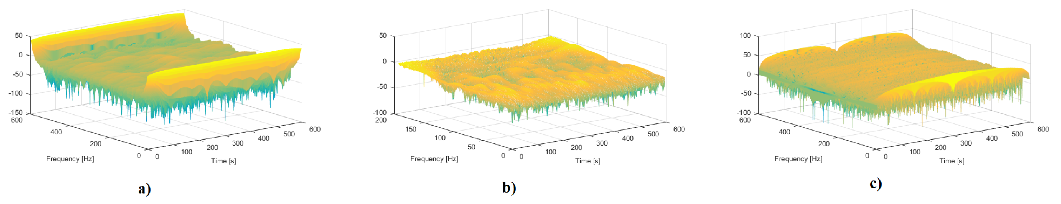
The next figures give examples of comparative representations of measured signals obtained from the aforementioned 28,000DWT bulk carrier. The figures represent the examples of time and TF domain representations of real-life ship pitch and roll motion response measurements. Firstly, in
Figure 9, the measured pitch and roll motion responses in the time domain are given with the duration of one dataset of 60 min.
Figure 10 and
Figure 11 give the representation of the pitch and roll motions in the TF domain using spectrogram, scalogram, and WVD representation methods. Simultaneous representation of the signal distribution in the time and frequency domain obtains a better characteristics extraction of measured signals. By comparing representations in the TF domain, one can see that there is a similarity between distributions. However, each has its advantages and disadvantages as mentioned before. WVD achieves the best clarity and frequency resolution, but for the multi-component signal, like these, it introduces much more interferences. On the other hand, these cross-terms interferences are eliminated on the spectrogram and scalogram representations, but their resolution is worse.
By combining and adapting existing feature extraction methods of various techniques, it is possible to enhance the accuracy of DP systems. If any of the distributions do not meet the application requirements, then it is necessary to either combine or adapt the existing fundamental methods that are described before and shown as examples in the figures. Adapting the appropriate TF distribution method for use in the signal filtering process can make a scientific contribution in terms of improving the accuracy of the estimation algorithm in dynamic positioning systems. After adequate processing and filtration of the measured motion signals and with knowledge of the complex RAO transfer functions, it is possible to obtain more accurate information on the DWS by combining ship motions for different encounter angles and encounter frequencies.
6. Kalman Filtering Techniques
Position, direction, and speed measurements in navigation systems are based on data collected from various sensors that are sensitive to noise and error. To estimate the information about forces and moments acting on the hull of a ship successfully, it is essential to detect and correct sensor errors, taking into account the measurement models of waves, wind, and sea currents [
9,
18]. For this purpose, an advanced filtering technique based on KF model can perform the filtration of the oscillatory wave-induced forces from the noisy signal measurements and provide optimum estimated states.
When designing a KF system model, it should be observable to achieve the convergence of the estimated states to the probabilistic expected value. State estimation is done by multiplying the prediction and measurement probability functions together, scaling the result, and computing the mean of the resulting probability density function. Optimum states can be reached with the minimization of the error variation by using a combination of various sensors and a feedback loop [
14]. The optimum state, in terms of the minimum error covariance, provides the ability to estimate the state of the dynamic system from the input-output pair in the feedback loop. A block diagram of such a system model is given in
Figure 12. The main idea is to control the error between the measured and the estimated values at zero with variable gain. In the model, noisy measurements are taken as a feedback signal based on which the estimation is made.
Computationally, the multiplication of these probability density functions relates to the discrete KF equation designed for stochastic systems, which is similar to the state observer for deterministic systems [
14,
15,
22,
51]:
The state vector contains information about the position, direction, and speed, and these variables should be estimated. It represents the a priori state, while the vector represents the a posteriori state. The variables to be estimated are given by matrices A (state transition matrix) and B (control matrix). The variable represents the input from which the estimate is derived, and takes into account the noise. KF is a two-step algorithm. It consists of a prediction part (time update equations) and an estimation part (measurement update equations).
Firstly, after measurements are taken, the prediction part is done. The linear system model, without dynamic noise taken into account, is used to calculate the a priori state estimate
and the error covariance
P:
The a priori error covariance matrix P is based on knowledge about the difference between measured states and previously estimated states. Matrix Q is the system process noise covariance matrix, defined in time intervals. It collects data about unmeasured dynamics and sensor noise.
The second part of the algorithm uses the a priori estimates calculated in the prediction step and updates (correct) them to find the a posteriori estimates of the state and to minimize error covariance. The state estimate of correction is given by:
where
H is a measurement matrix related to the connection between the current state and measurement. The expression
represents the deviation of the actual
measurement from the predicted measurement. The Kalman gain
is calculated so that it minimizes the a posteriori error covariance:
where
R is the measurement noise matrix.
Once the update equations are calculated, in the next time step, the posterior estimates are used to predict the new a priori estimates, and the previous steps are repeated. To estimate the current state, the algorithm does not need all past measurements. Only estimated states, the error covariance matrix from the previous time step, and the current measurement are needed. In other words, the KF is a recursive method. However, the recursive form is not the best choice for real-time implementations because of the problem of numerical calculations of covariance matrices. By quadratic filtering, better accuracy and stability can be achieved [
14,
22].
The KF is essentially linear, so it is necessary to linearize (approximate) the complex nonlinear equations of the DP system to remove noise. Such calculations represent a strain on the system since the calculation of parameters should be obtained in real time. Furthermore, the KF is driven by white noise, which further contributes to the problems and limitations of achieving an accurate estimation [
22,
52].
More accurate approximation of nonlinear systems can be done by utilizing the extended Kalman filter (EKF). EKF performs linearization of the nonlinear function around the mean of the current state estimate. This formulation also performs calculations of the Jacobians matrices and tunes the gain while updating the states using a linear function. However, EKF has some drawbacks. There is a problem in the calculation of the Jacobians analytically due to complicated derivatives and the high computational cost to calculate them numerically. Furthermore, a system with a discontinued model is not differentiable, and Jacobians do not exist [
51]. To allow the Jacobian’s free estimation, Alminde et al. (2007) [
53] studied the application of integrated quantized state simulation to propagate the state and obtain a backward variance estimate of the Jacobian and ultimately confirmed their theory. The EKF algorithm proved to be satisfying in numerous marine navigation applications. For example, Kuchler et al. (2011) [
54] confirmed the improvement in the estimation of the heave motion using the acceleration measurements and EKF filter. Furthermore, Assaf et al. (2018) [
55] in their study extended the use of EKF to discuss more general nonlinear estimation problems. The proposed algorithm was shown to be effective in tracking normal ship speed.
When the linearization procedure does not provide a fine approximation for highly nonlinear systems, another estimation method called the unscented Kalman filter (UKF) is used. Instead of approximating a nonlinear function as EKF does, such filters approximate the probability distribution [
9,
51,
52]. The algorithm is based on Bayesian theory and the deterministic sampling technique, also known as unscented transform (UT). Shown in
Figure 13, the filter selects a minimal set of sample points (also referred to as sigma points and symmetrically distributed around the mean) from the Gaussian distribution, and it propagates them through the nonlinear system model. By utilizing the UT transform, it estimates the mean and covariance values of the new transformed sample point dataset and uses them to find the new state estimates. UKF is not robust to a non-Gaussian environment with outliers, and there is a need for a different robust solution. In their study, Peng et al. (2019) [
9] proposed modified UKF to reduce the influence of outliers on estimates. In the proposed study, they confirmed the improvement in terms of stability, convergence properties, an accurate estimation of all given states.
Research of Vaernø et al. [
8] gave an overview of dynamic algorithms for ship positioning with four different control models, including the linear KF, EKF, and UKF. The results confirmed that the DP process was predominantly linear. Slight improvement in performance can be achieved by using nonlinear damping (namely by including the EKF or UKF algorithms). Linear KF behaves similarly to EKF and UKF only when linear damping is used. The control implementation and observation algorithm largely depend on how well the underlying model embraces the dynamics of the system. Furthermore, a detailed description of the high confidentiality model with various models of controller and observer designs was given by Fossen (2011) [
15] and Sorensen (2011) [
56].
Another nonlinear state estimator, based on a similar principle, is the non-parametric approximation technique called the particle filter (PF). It also uses sample points referred to as weighted particles. The flow of a set of particles from the prediction phase through the update phase to the resample phase and back to the prediction phase, with a non-parametric representation of the distribution density, is shown in
Figure 14.
This filter can approximate any arbitrary distribution, and it is not limited to a Gaussian noise only. It is based on the Monte Carlo method, and approximation is done using the probability density function with the sample mean instead of the integral operation [
52]. The more accurate approximation is obtained by use of more particles. On the other hand, in relation to UKF, it is a computationally expensive filter since it requires a larger number of particles to represent a distribution not known explicitly [
57]. Furthermore, the problem of particle sample degradation occurs due to the variation of particle weight, increasing with the iteration time. This leads to inefficient use of resources and the decreased efficiency of approximation. Due to the structural complexity and computational cost, these types of filters are not often used in control systems, but their development and improvements in recent years are increasingly discussed.
Important characteristics to consider when designing a filter are computational complexity and efficiency, estimation accuracy, and robustness. A comparative overview of these characteristics for KF, EKF, UKF, and PF is given in
Table 3.
The combination of PF and KF can be called the particle KF. In doing so, PF is used for noise filtering, and KF is used to observe unmeasurable states. Changing the window width and the number of samples can affect the performance of such a filter. In another work, Jaros et al. (2018) [
58] provided a comparative analysis of two particle KF formulations based on a kinematic model and/or a dynamic ship model. Similarly, Chen et al. (2018) [
52] in the proposed algorithm used PF as a framework and additionally UKF as a density function for particle state optimization. This approach has proven satisfactory in terms of estimating the low-frequency oscillation of the ship.
In general, KF-based techniques demonstrate the ability to evaluate progressively the states using multi-sensor fusion, take the forward speed into account, are very effective in real-time estimations, and can evaluate measurements even when they are not available. On the other hand, the problem of smoothing, computational cost, and not sufficiently good estimation for the cases of individual performances depending on the data create disadvantages with these techniques and need to be further investigated. Research into the best combination of the described Kalman filter variations remains open, and it would be advisable to emphasize the possibility of finding an innovative solution that can be based on the complementarity of filtering algorithms (for noise filtering) and artificial intelligence algorithms (for predicting upcoming conditions).


