Article

Oil Droplet Dispersion under a Deep-Water Plunging Breaker: Experimental Measurement and Numerical Modeling

1
Center for Natural Resources, Department of Civil and Environmental Engineering, New Jersey Institute of Technology, Newark, NJ 07102, USA
2
Department of Fisheries and Oceans, Bedford Institute of Oceanography, Dartmouth, NS B2Y 4A2, Canada
*
Author to whom correspondence should be addressed.
J. Mar. Sci. Eng. 2020, 8(4), 230; https://doi.org/10.3390/jmse8040230
Submission received: 1 March 2020 / Revised: 21 March 2020 / Accepted: 23 March 2020 / Published: 25 March 2020
(This article belongs to the Special Issue Marine Oil Spills 2020)

Abstract

:
Knowledge of the droplet size distribution (DSD) of spilled oil is essential for the accurate prediction of oil transport, dissolution, and biodegradation. Breaking waves play important roles in oil droplet formation in oceanic environments. To understand the effects of breaking waves on oil DSD, oil spill experiments were designed and performed in a large-scale wave tank. A plunging breaker with a height of about 0.4 m was produced using the dispersive focusing method within the tank. Oil placed within the breaker resulted in a DSD that was measured using a shadowgraph camera and found to fit a Gaussian distribution N (µ = 1.2 mm, σ2 = 0.29 mm2). For droplets smaller than 1500 µm, the number-based DSD matched the DS1988 correlation, which gives N(d) ~ d−2.3, but this was N(d) ~ d−9.7 for droplets larger than 1500 µm. An order of magnitude investigation revealed that a Gaussian volume-based DSD results in a number-based DSD that may be approximated by d−b (with b ≈ 2) for small diameters (relative to the mean), which explains the occurrence of the DS1988 correlation. With the measured wave hydrodynamics, the VDROP model was adopted to simulate the DSD, which closely matched the observed DSD. The present results reduce the empiricism of the DS1988 correlation.

1. Introduction

Predicting the dispersion of oil droplets in the water column is of major importance to assess the impact of oil spill on the ecosystem and communities [1]. For oil released on the ocean surface, breaking waves play an important role in the dispersion and fate of oil spills. A schematic illustration of the dispersion of oils under breaking waves is shown in Figure 1. The released oil films float on the water surface due to the buoyancy. After getting hit by the breaker, the oil films break up into droplets of different sizes due to the dynamic pressure and multi-scale turbulence engendered by the breaking wave [2,3]. The large-size droplets tend to stay at the water surface and transport forward rapidly following the drift velocity of the surface waves, while the small-size droplets may be entrained into the deep water column due to small rise velocities and the wave turbulence. The resulting droplet size distribution (DSD) by the breaking wave mainly depends on two factors, namely the wave energy and the oil resistance forces. The two resistance forces are the oil–water interfacial tension (IFT) and oil viscosity, which prevent the oil films/droplets from breaking up. When the wave energy induced by the turbulent fluctuation exceeds the resisting forces, oil films/droplets burst into smaller droplets. The higher the wave energy, the smaller the oil droplets that can be formed.
Understanding the effects of breakings waves on the dispersion of oil slicks at seas is a challenging task, as the environmental conditions are very complex and it is not possible to have sufficient measurements to gain a predictive relationship between the sea state (i.e., wave heights) and the oil droplet dispersion in the water column. This has led to extensive wave flume experiments to study the oil entrainment and droplet size distribution (DSD) in the water column. The best-known experiment was performed by Delvigne and Sweeney [4], henceforth DS1988, in various wave tanks. The DS1988 reported that the number of droplets of a given size is proportional to that diameter to the power 2.3. Thus, the number of submerged oil droplet increases with a decrease in diameter. The DS1988 experiments focused on the role of oil viscosity, and the range of oil–water interfacial tension considered was very narrow (0.019 N/m to 0.03 N/m) and thus does not account for the application of chemical dispersant.
Following DS1988, experiments with various oils and dispersants were conducted at a wave tank located at the Bedford Institute of Oceanography, Canada [5,6,7,8]. They found that the volume-based oil droplet size distribution is lognormal in the absence of dispersant and bi-modal in the presence of dispersant. Efforts for modeling those data were conducted by Boufadel et al. [9] and Chen et al. [10]. Recently, Li et al. [11] reported experimental results of oil dispersion due to a plunging breaker of a solitary wave without and with dispersant. Their results indicated that, in the absence of dispersant, the model reported in DS1988 holds well for entrained droplets whose diameters are smaller than 1000 µm, but that it overestimates the number of submerged larger-sized droplets.
Tremendous effort has also been spent on developing numerical models for DSD based on oil properties and hydrodynamic environments [12]. Models for the droplet size distribution range from correlations to detailed simulations of DSD. Correlation models rely on dimensionless numbers, such as the Weber number—a ratio of destructive forces to resisting forces due to interfacial tension (IFT)—and the Reynolds number to obtain a characteristic diameter, namely the volume-median diameter, d50, at steady state (i.e., after a long time of mixing). A salient work on the topic was produced by Johansen et al. [13], who also proposed a correlation model for oil entrainment using non-dimensional groups. They also accounted for situations in which the oil viscosity resists breakup [14] through the incorporation of the so-called modified Weber number [15]. Li et al. [16] developed a variant of the approach put forward by Johansen et al. that included the usage of the Ohnesorge number in the correlation.
Population balance models rely on solving differential equations numerically for the whole equilibrium and transient droplet size distribution (DSD) (i.e., not only the d50 and not only at equilibrium). The models take account of various mechanisms causing breakup and the coalescence of droplets in a mechanistic way along with mechanisms resisting breakup [17,18]. Zhao et al. [19] developed and validated a population dynamic model, VDROP, and this has been successfully used in many scenarios [20,21] and is adopted in the present study.
One major purpose of this study is to develop an experimental approach for in-situ measurements of oil droplet size distribution under breaking waves in large laboratory/outdoor wave tanks. Additionally, the study is motivated by studying the power–law correlations reported in the published literature and finding mathematical or physical interpretations of them. Finally, this study aims to extend the application of the VDROP model to simulate the DSD under wave conditions. In the present study, breaking wave experiments were performed in a flap-type wave tank at Bedford Institute of Oceanography in Canada. A plunging breaker with a height of 0.4 m was generated using the dispersive focusing method [22] within the wave tank. The hydrodynamic properties of the breaker (i.e., water elevation, velocity components) were measured and used to estimate the energy dissipation rate. The DSD of entrained oil was measured using a shadowgraph camera (discussed below) and compared with the correlation reported by Delvigne and Sweeney [4] and Li et al [11]. With the estimated energy dissipation rate, the population balance model VDROP was used to numerically compute the oil DSD, and the results are compared with the experimental measurements. A parametric study of the VDROP model was also performed with different energy dissipation and time durations.
The paper is organized as follows: In Section 2, we present our methodology along with the details of the experimental setup and numerical model. In Section 3, we report our results of wave hydrodynamics and droplet size distribution. A discussion will be given in Section 4 regarding the obtained results, and a conclusion is presented in Section 5.

2. Methodology

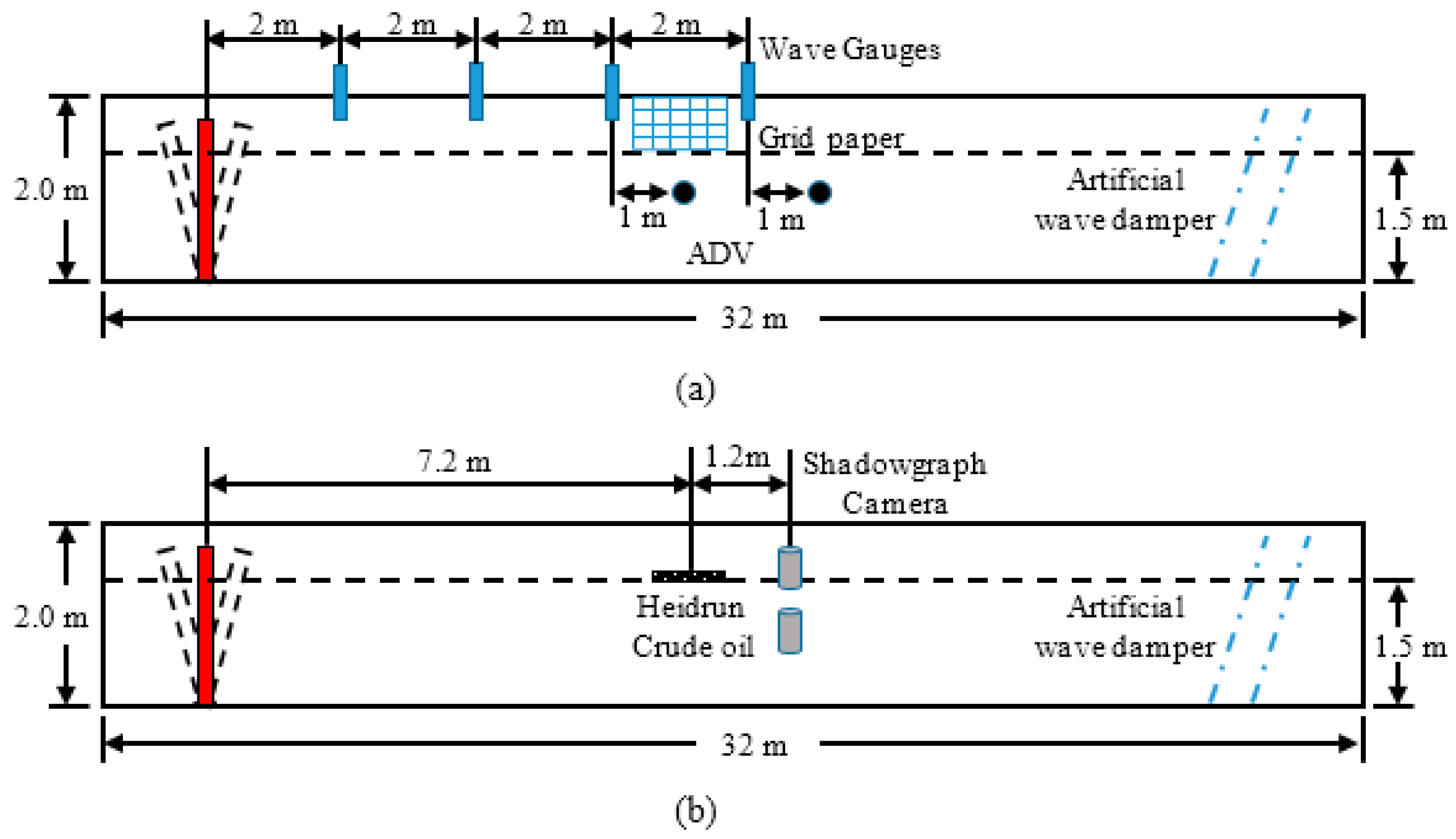
2.1. Experimental Approach

The experiments were conducted in a wave flume located in Bedford Institute of Oceanography (BIO), Nova Scotia, Canada in June 2019, which has the following dimensions: 32 m long, 0.6 m wide, and 2.0 m tall. The tank was filled with seawater to a depth of 1.5 m during the experiments. Waves were created using a flap-type wavemaker, hinged at the bottom [23,24]. The temperature of the water was 15 °C. Two types of experiments were performed, namely the breaking wave experiment and oil dispersion experiment.
In the breaking wave experiments, a deep-water plunging breaker was generated using the dispersive focusing method [22,25], where the wave energy was focused longitudinally by linearly decreasing the wave frequency; thus, the group velocity of the generated waves increased, leading to a dispersive focusing of the waves. The designed wave packet was composed of 32 linear wave components with different frequencies and wavelengths, similar to the laboratory experiments by Rapp and Melville [26], Drazen et al. [27], or the recent numerical simulations by Derakhti et al. [28]. At the wave paddle (x = 0 m), the horizontal and vertical velocities are given by
u ( x = 0 , z , t ) = n = 1 32 2 π f n a n cosh k n ( h + z ) sinh k n h cos [ k n x b 2 π f n ( t t b ) ]
and
w ( x = 0 , z , t ) = n = 1 32 2 π f n a n sinh k n ( h + z ) sinh k n h sin [ k n x b 2 π f n ( t t b ) ]
where a n is the wave amplitude, f n is the wave frequency and k n is the wavenumber. The x b and t b are the expected focal point and breaking time, respectively. The water depth h was 1.5 m in the present study. Based on the horizontal velocities, the horizontal positions of the wave paddle at the mean water level could be calculated, which were subsequently converted to a voltage profile used as the input for the electric motor. The parameters of the wave components and the voltage profile are shown in Table A1 and Figure A1, respectively (see Appendix A). Sonic wave sensors (Ocean Sensor System) were used to measure the water elevation at x = 2, 4, 6, and 8 m from the wave paddle. The error of the sonic wave sensors was less than 1 mm, and the sampling rate was 32 Hz; as the smallest wave period was 0.8 s, the wave gauge allowed a good capture of the water surface. A sheet of waterproof grid paper was placed on the sidewall of the wave tank from x = 7 to 8 m facing a GoPro Camera fixed on the opposite sidewall to allow water elevation (and wave height) measurement based on the camera videos. Two Acoustic Doppler Velocimetries (ADV, Nortek) were deployed at x = 7 and 9 m at two different elevations of 131.15 cm and 127.5 cm, which were 18.5 and 22.5 cm below the 1.5 m level, respectively. The ADV also output the signal-to-noise-ratio (SNR) and correlations, which were used to evaluate the quality of the data. The schematic illustration of the breaking wave experiment is shown in Figure 2a.
Heidrun crude oil was used in the test, which has a density of 912.8 kg/m3 and a viscosity of 68.9 cSt at 15 °C [29]. The oil–water interfacial tension was 17.4e-3 N/m. About 100 grams of Heidrun crude oil was placed as a film in a ring 7.2 m from the wave paddle in the breaker zone. A shadowgraph camera was deployed 1.2 m downstream of the oil film and 10 cm below the mean water level 1.5 m to take the images of the dispersed oil droplets. The measurement window of the shadowgraph camera was 4 × 5.5 cm with a resolution of 13.5 µm. Based on the camera resolution, droplets larger than 150 µm could be well captured. The schematic illustration of the oil dispersion experiment is shown in Figure 2b. The open-source software ImageJ was used to process the images taken by a shadowgraph camera. ImageJ is a Java-based image process program developed by the National Institutes of Health (NIH), and it has been widely used in various scientific fields [30]. The oil spill experiment was performed twice to check the repeatability of the experimental data.

2.2. Numerical Approach

The energy dissipation rates are usually evaluated based on turbulent velocities, as the spatial gradient of the average velocity is negligible in the presence of turbulence [31,32]. In this work, the turbulent velocities at each location were obtained as the deviation of the measured fluid velocity from the moving average velocity at that location as follows:
u n ,   t = u n ,   t u ¯ n ,   t   ,   and   n = x ,   y ,   z
where t indicates different time points, u t is the measured velocity, u t is the turbulent fluctuation velocity components, and u ¯ t is the moving average velocity at each time point obtained as follows:
u ¯ n , t = k = t p 1 2 k = t + p 1 2 u n , k p   ,   and   t = p + 1 2 ,   p + 3 2 ,   p + 5 2 , , ( N p 1 2 )
where N is total the number of time points and p is the number of points used for the average. The increase in p smooths the series, and choosing odd (versus even) p values provides symmetry around the current time value using the same number of values before and after the current time during the averaging. In the current study, p was taken to be 5. Therefore, the energy dissipation rates can be calculated as
ε n , t = ( u n , t ) 2 d t ,   and   n = x , y , z
where d t is the sampling time interval, which was equal to 0.02 s.
The population balance model VDROP [19] was used to numerically compute the droplet size distribution. The number concentration of droplets of size d i , n ( d i , t ) in (number of droplets/m3), evolves as
n ( d , t ) t = g ( d i ) n ( d i , t ) + j = i + 1 n β ( d i , d j ) g ( d j ) n ( d j , t ) Droplet   Breakup + j = 1 n k = 1 n Γ ( d j , d k ) n ( d j , t ) n ( d k , t ) n ( d i , t ) j = 1 n Γ ( d i , d j ) n ( d j , t ) Droplet   Coalescence ( V j + V k = V i )
where n is given as a number of droplets/m3, d i is given in meter at a given time t (seconds). The function g ( d j ) is the breakage frequency of droplets of diameter d j (reported below). The first term on the RHS (right-hand side) of Equation (6) represents the death of droplets of size di. The term β ( d i , d j ) is the breakage probability density function (dimensionless) for the creation of droplets of diameter d i due to the breakage of droplets of (a larger) diameter d j [33]. This represents the fact that droplets have a larger tendency to break into two unequal parts, as that produces the smallest oil–water surface area. Note that we are assuming that two daughter droplets result from a breakup. The second term on the RHS of Equation (6) represents the birth of droplets d i resulting from the breakup of droplets of a size d j larger than d i . For droplet coalescence, the term Γ ( d k , d j ) is the coalescence rate (m3/s). The first term of droplet coalescence represents the birth of droplets d i as a result of coalescence events occurring between droplets d k and d j to form droplets with the size of d i , while the second term represents deaths of droplets d i due to the coalescence of droplets of size d i with all other drops (including drops of size d i themselves) to form larger droplets. The VDROP model accounts for both the effect of oil viscosity and the oil–water interfacial tension on oil droplet formation. The functionality of   g ( d j ) , β ( d i , d j ) , and Γ ( d k , d j ) has been thoroughly discussed in Zhao et al. [19] and thus is not addressed here. Inputs to the model VDROP include the oil properties, oil–water interfacial tension, the energy dissipation rate, and the duration of the breakup (and coalescence).

3. Results

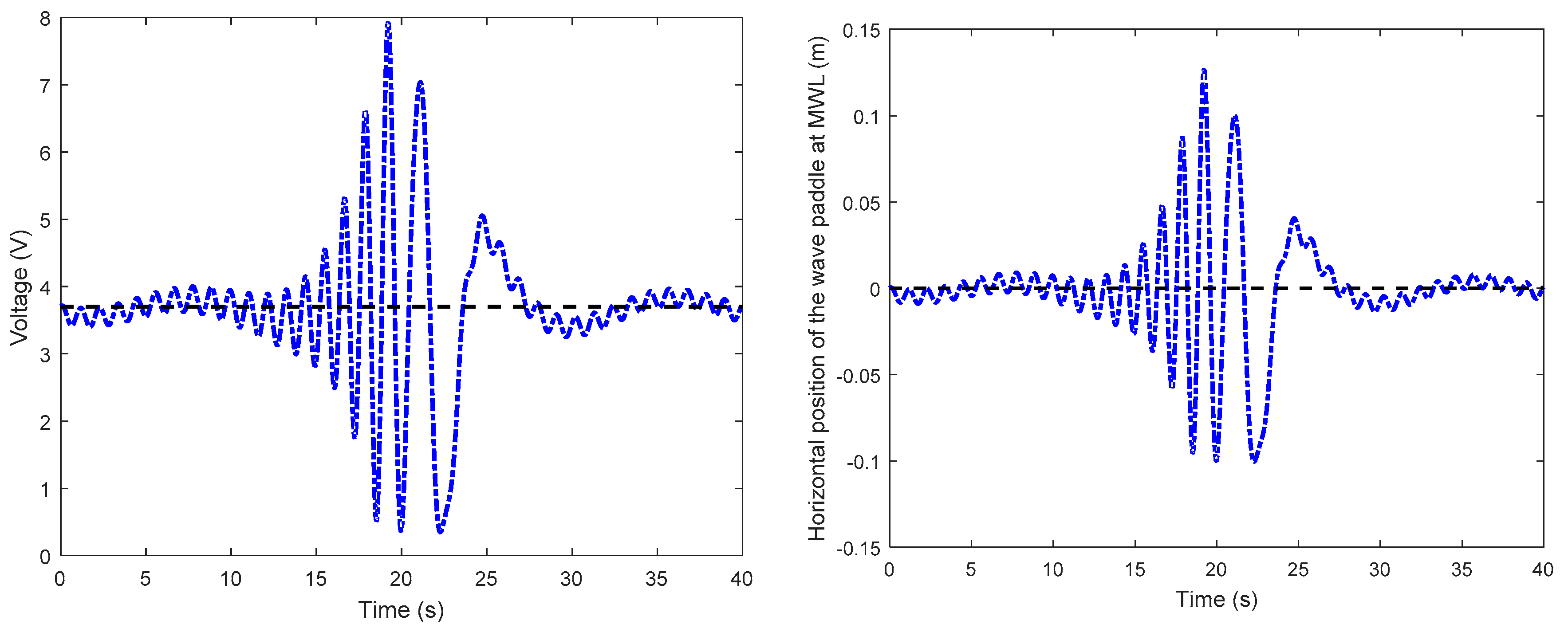
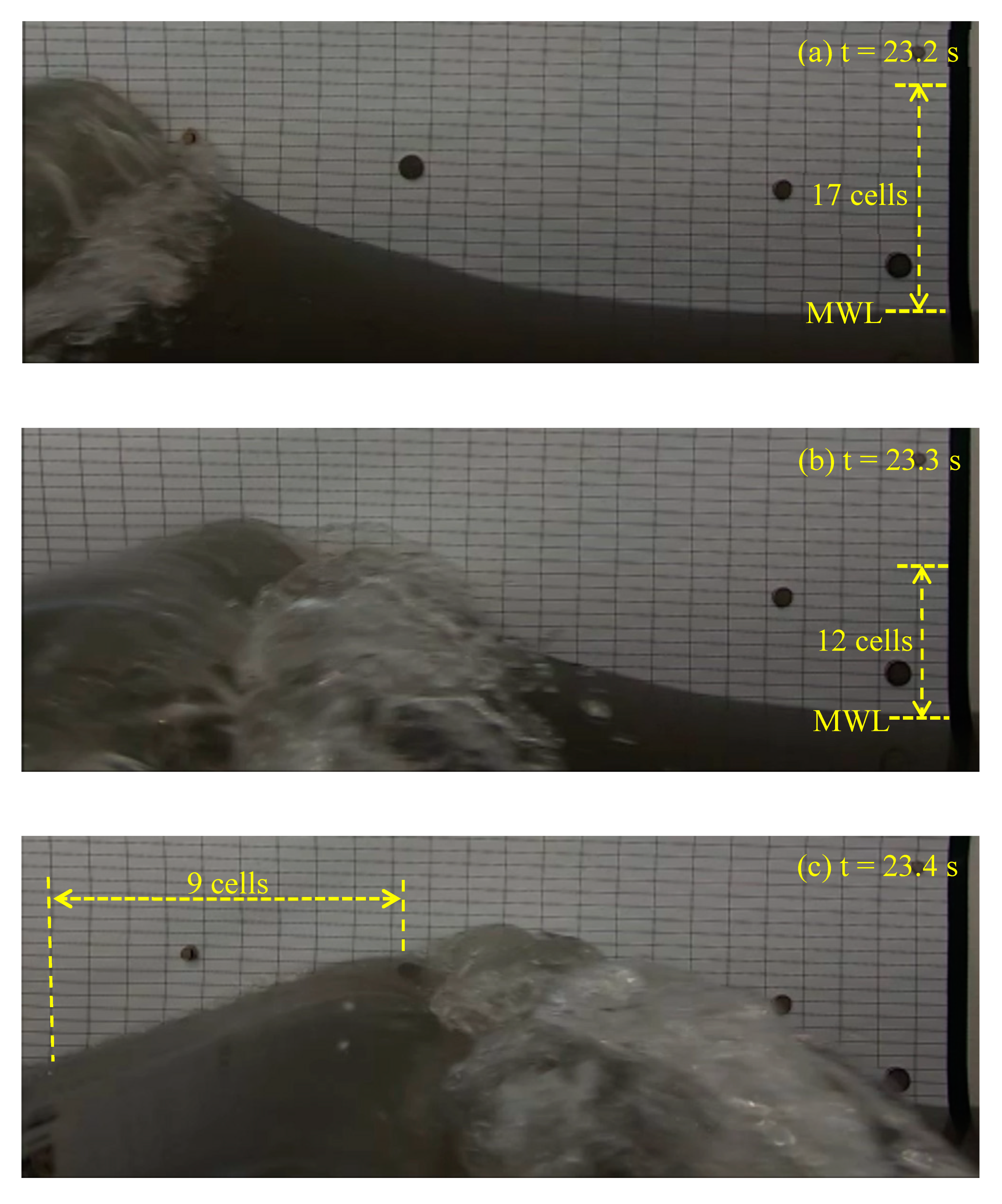
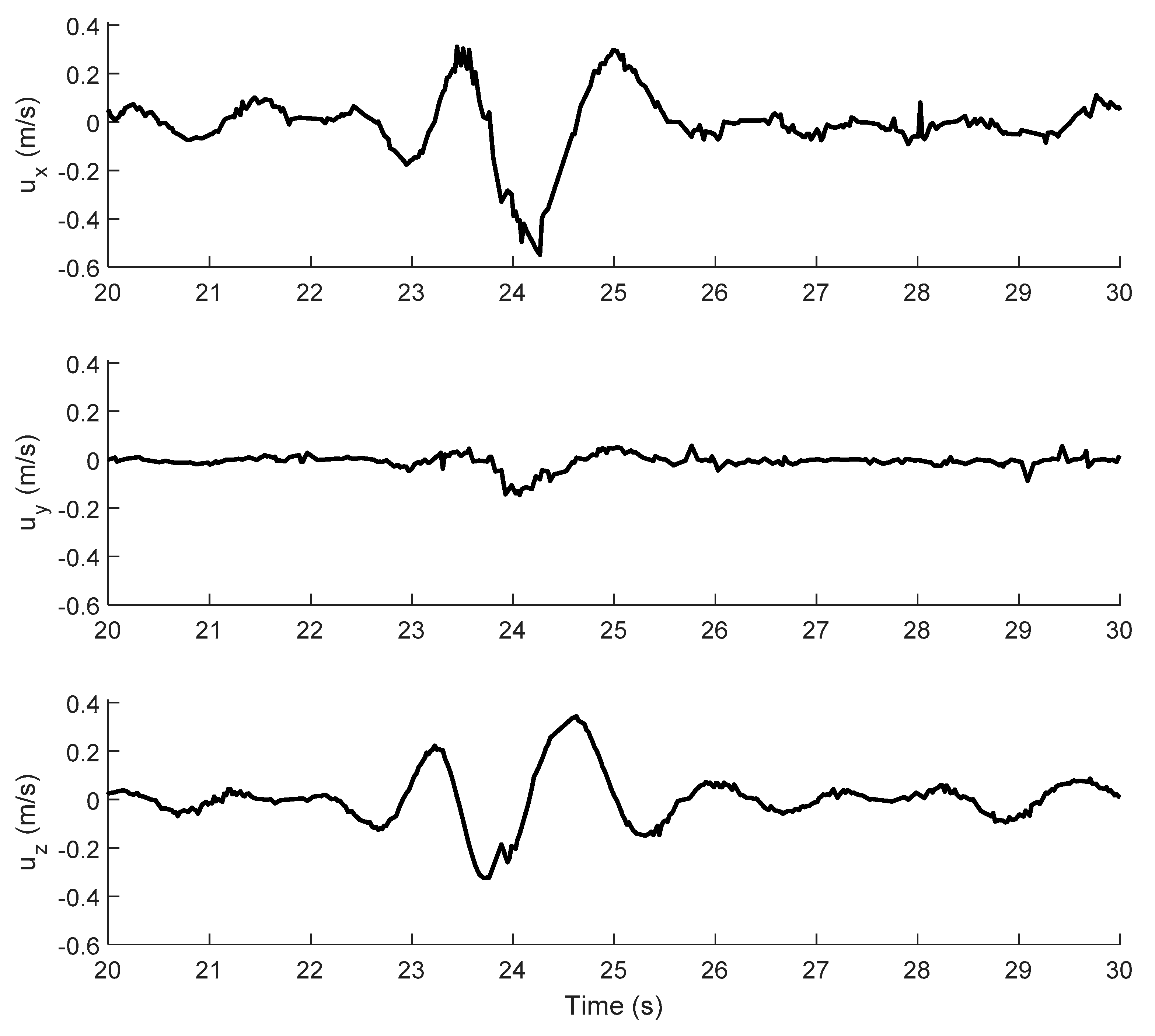
3.1. Characterization of the Plunging Breaker

The generated plunging breaker occurred at x o b = 7.1 m and t o b = 23.2 s, which were close to the designed focal location and time ( x b = 7.0 m, t b = 25 s). Figure 3 shows the front images of the breaking wave, which were taken by the GoPro camera. A large, steep wave crest was observed at t = 22.7 s (Figure 3a) due to the focusing of the wave components. The wave crest advected faster than the wave, and an overturning jet occurred and fell on to the water surface, which led to the formation of a plunging breaker (Figure 3b). The plunging breaker retained a large amount of energy and caused a water splash-up, which subsequently resulted in a secondary breaker (Figure 3c). The wave kept propagating forward after breaking, and the water surface started to recover at t = 23.9 s (Figure 3d). “Whitecaps” were observed during the breaking process, which are small bubbles formed by the entrained air due to the breaking wave.
Figure 4 shows side views of the breaking wave, which were taken by the GoPro camera. Each cell on the grid paper has a dimension of 3.85 (L) × 1.3 (W) cm. It is shown in Figure 4a that the wave height was about 22.1 cm (17 cells) when the overturning jet hit the water surface at t = 23.2 s. The water splash-up caused by the major plunging breaker at t = 23.3 s had a height of about 15.6 cm (12 cells) (Figure 4b). The wave propagated forward about 35 cm (9 cells) within 0.2 s, which corresponds to a phase speed of 1.75 m/s. The successive impingement between the breakers and water surface caused a large number of water ligaments and “white caps” (Figure 4a–c).
Figure 5 shows the temporal evolution of water levels at different locations measured by the sonic wave sensors. It can be observed that there were three large wave crests which passed through x = 2 m from t = 18 to 22 s. The number of wave crests which passed through x = 4 m decreased, but the wave crests became higher and steeper, which reflected the focusing process of the wave components. A very steep high wave crest was observed at x = 6 m around t = 22.7 s, which led to the occurrence of the plunging breaker at t = 23.2 s (indicated by the red dashed line; see also Figure 4a,b). The wave height (maximum distance between trough and following crest) was around 0.40 m before breaking (x = 6 m). The water elevation at x = 8 m shows that a large wave crest propagated following the breaking wave, and the water surface recovered afterwards. The water elevations at different locations clearly show the propagation and focusing process of the waves.
The velocity components under the plunging breaker (at x = 7 m, and 23.5 cm below the mean water level 1.5 m) measured by Acoustic Doppler Velocimetry (ADV) are shown in Figure 6. The velocities were relatively small in each direction before the occurrence of the plunging breaker. Large velocity fluctuations were observed in the horizontal and vertical direction after the occurrence of the plunging breaker (t > 23 s). The maximum forward velocity was about 0.3 m/s, and the backward velocity reached up to −0.6 m/s, which indicates a strong backflow caused by the breaker. A phase shift was observed between horizontal and vertical velocities. The fluctuation of the vertical velocities ranged from −0.3 to 0.3 m. After the passage of the wave train (t > 27 s), the velocities in each direction rapidly decayed. The velocities in the cross-tank direction were much smaller than the other directions during the whole test, which reflects the fact that the hydrodynamics of the breaker were nearly 2D. Other sets of measured velocity data can be found in the Supplementary Materials.

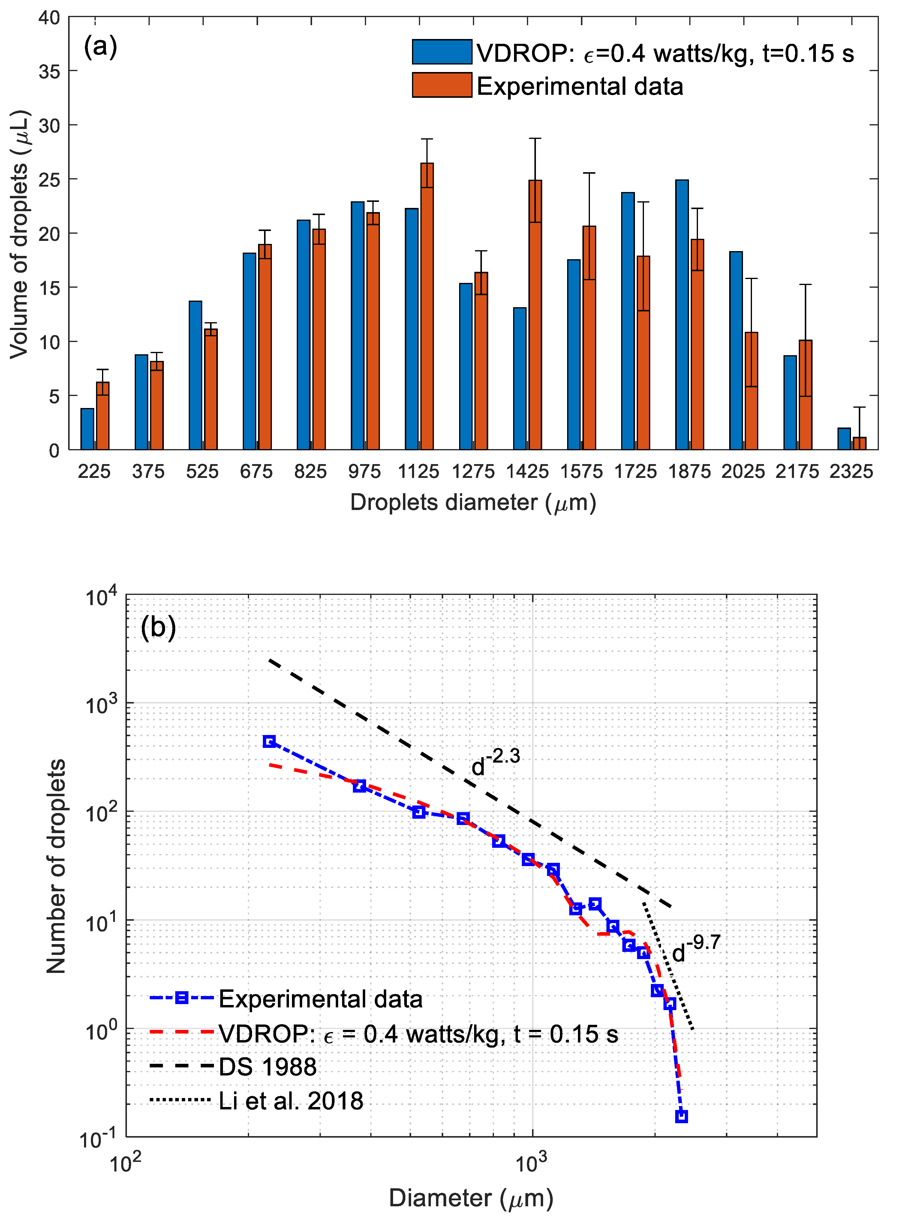
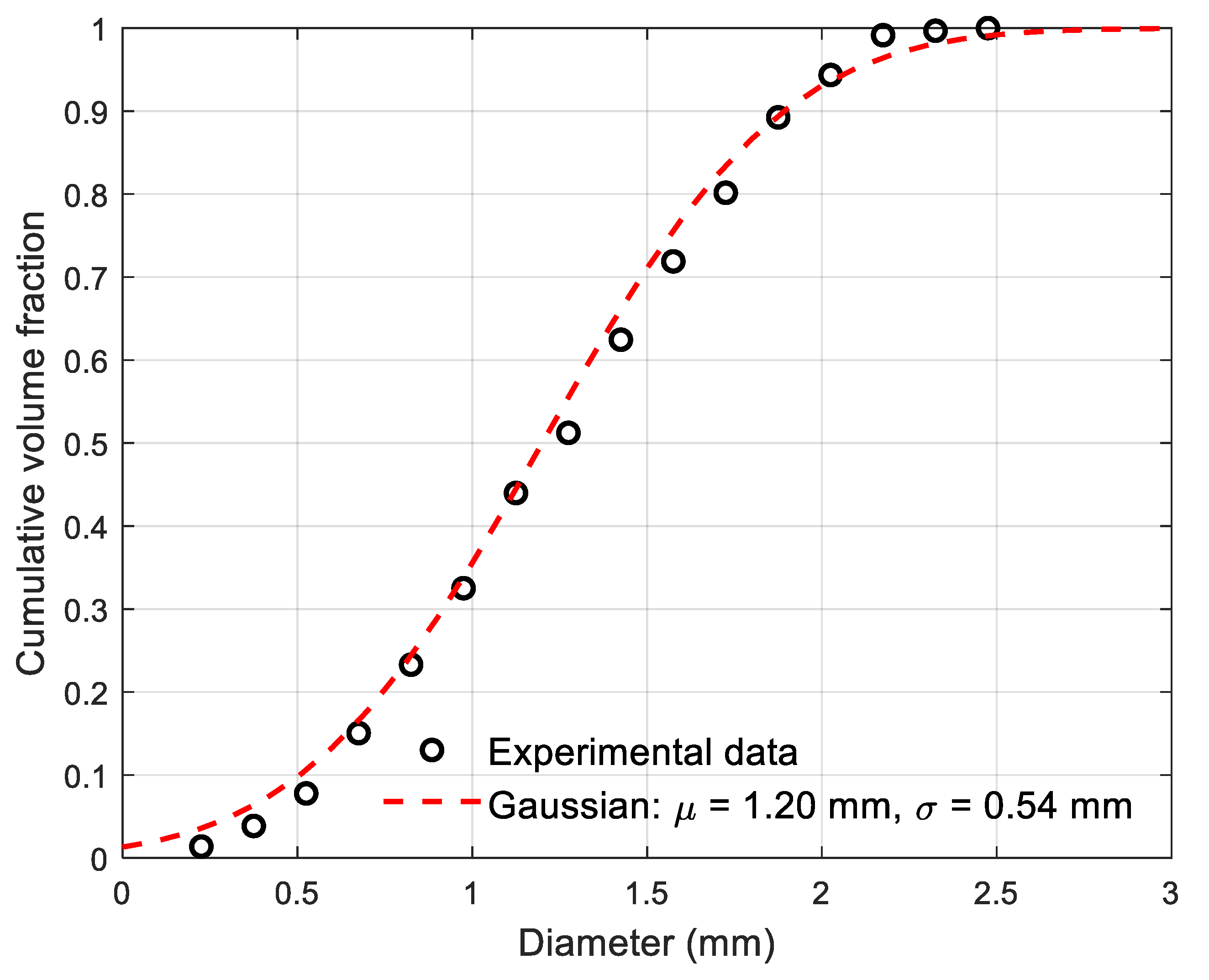
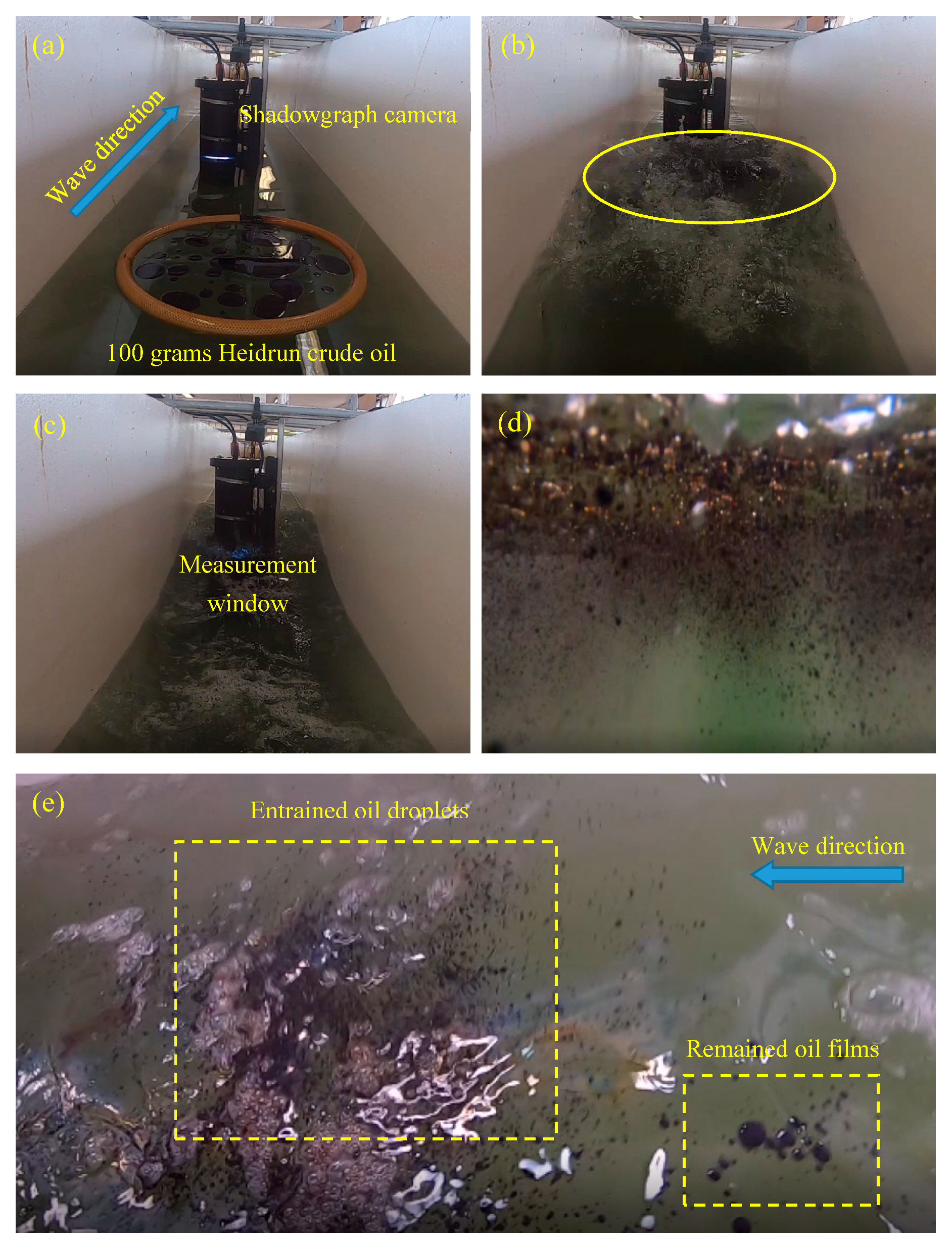
3.2. Oil Dispersion under the Plunging Breaker

Figure 7 shows the snapshots of the oil dispersion experiments taken by the GoPro camera. The experiment setup before starting the wave paddle is shown in Figure 7a. One hundred grams of Heidrun crude oil was released at x = 7.2 m, and the shadowgraph camera was deployed 1.2 m downstream of the crude oil (see also Figure 2b). A plastic O-ring was used to prevent the oil from spreading, which was taken out of the tank right before the occurrence of the plunging breaker. The oil films dispersed into oil droplets after being hit by the plunging breaker (Figure 7b within the yellow circle), and the dispersed oil droplets were transported downstream to the measurement window of the shadowgraph camera with the propagation of the wave (Figure 7c). An underwater view of the dispersed oil droplets taken by a GoPro camera is shown in Figure 7d, which demonstrates that droplets of various sizes were entrained in the water column to different depths. Figure 7e shows a side view of the dispersed oil plume after the passage of the wave train. It appears in Figure 7e that a large number of oil droplets were formed and entrained into the water column, and several oil films remained in the water surface (see the yellow rectangles).
Figure 8 shows an example of the photos taken by the shadowgraph camera. The dark disks indicate the oil droplets of various sizes, while the hollow circles indicate the air bubbles. The background was removed by setting a threshold of the gray value. The air bubbles were eliminated manually or taken out during the statistical process by checking the mean gray value (i.e., the mean gray value of a dark sphere is 255, and otherwise the value is less than 255) and circularity. The clustered droplets were broken up using the Watershed algorithm provided by ImageJ. Due to the resolution of the shadowgraph cameras, only droplets larger than 150 µm were considered during the analysis. The obtained droplet sizes were assigned to different size bins to form a droplet size distribution (DSD). The droplet size bins ranged from 150 to 2400 µm with a 150 µm interval. Thirty photos after the passage of the wave train (t = 35–38 s) were analyzed to obtain a temporally averaged DSD.
Figure 9 shows the volume and number of droplets in each size bin provided by ImageJ using the photos taken by the shadowgraph camera. The median value of a size bin was used to represent the bin in the results (i.e., we use 225 µm to represent a droplet bin of 150–300 µm). The captured volume-based DSD seemed to be bimodal (Figure 9a). The standard deviation significantly increased for droplets larger than 1500 µm, which reflects the fact that the number of these droplets was generally small (but their volume was not). The volume-based DSD in Figure 9a was found to fit a Gaussian distribution ( N (µ = 1.2 mm, σ2 = 0.29 mm2)) at the 5% significance level by the Kolmogorov–Smirnov test [34]. The volume-based DSD is plotted on a normality sheet in Figure A2, and the cumulative volume-based DSD was reported in Figure A3. A Gaussian distribution was observed in numerous studies of DSD in reactors [33,35,36]. Section 4 addresses this point in more detail. Figure 9b shows the number of droplets as a function of the diameter in a log-log plot to allow comparison with the correlation reported in DS1988. The figure shows that droplets smaller than 1500 µm generally followed the DS1988 correlation given as N(d) ~ d−2.3. However, for droplets larger than 1500 µm, the number of droplets decreased much faster with the diameter and may be approximated by N(d) ~ d−9.7, as reported by Li et al. [11] based on their measurements of oil droplets following a plunging breaker. Figure 9 also reports the simulated DSD using the VDROP model, which will be discussed in the following paragraphs. A similar DSD was found in the repeat experiment, which proves the repeatability of the experiment. The DSD in the repeat experiment could also be well approximated by the reported power–law correlations (see Figure S3).
The energy dissipation rate ε in each direction was calculated based on Equations (3)–(5) using the measured velocities (Figure 6). The results are shown in Figure 10, and they display strong intermittency (sudden jumps), with high energy dissipation rates occurring mainly between 23 to 26 s, coinciding with the wave breaker. The energy dissipation rates in the horizontal (x) and vertical (z) directions were much higher than those in the cross-tank (y) direction, which reflects the two-dimensional nature of the wave motion (by design).
The breakup of oil droplets occurs at the µm-scale and within milliseconds (see the Discussion section of Zhao et al., 2014 Chemical Engineering Journal). In particular, it is well known that large ε values cause the breakup, but these occur over short durations (milliseconds and below) and cover only a small fraction of the volume. The latter has formed the basis for using a multifractal representation of ε, where the active or effective volume of mixing is only a small fraction (less than 5%) of the total volume [37,38,39]. A discussion in the context of oil dispersion was also presented in more recent works [9,40]. In our case, we needed to use a “design” or representative value of the energy dissipation rate ε to integrate the temporospatial interaction of the hydrodynamics and the oil plume. This is similar to the concept of the significant wave height in coastal engineering used as a design parameter for structures [41,42], where the significant wave height is obtained as the average of the top one-third of wave heights. For this reason, we used the average of the top 30% of the ε values during the breaker (i.e., from 23 to 26 s). This was done in each direction to obtain the design ε, labeled ε a v g , reported also in Figure 10. The values of ε a v g were 0.39 watts/kg along the tank (horizontal), 0.18 watts/kg vertical, and 0.07 watts/kg across the tank (horizontal).
As input to VDROP, the largest size of oil droplets observed in the experiment was 2400 µm (see Figure 9a) and was adopted as the maximum droplet size in VDROP simulations. The size bin interval was taken as 150 µm, which was the same as that used in processing the experimental results. As reported in Figure 10, the maximum ε a v g was equal to 0.39 watts/kg found in the horizontal direction along the tank. We elected to use the maximum value of the directions to characterize the breaker, which was due to the fact that breakage depends on the large values of ε in the field [43]. Thus, neither adding ε in the three directions nor taking the average of the three directions was correct. We used the value of 0.4 watts/kg and varied the duration of the breaking from 0.1 to 0.5 s with an increment of 0.01 s to match the observed oil DSD. Figure 9a shows that the agreement for the volume of oil droplets of each size is good for a duration of 0.15 s. The simulated number of oil droplets as a function of diameter also closely matched the observed results (see Figure 9b). The VDROP simulation moderately underestimated the number of 225 and 1425 µm droplets and slightly overestimated the number of 2425 µm droplets. However, the difference was within the level of uncertainty of the data.
We also conducted a sensitivity analysis study using energy dissipations of 0.2, 0.4, and 0.6 watts/kg for time durations of 0.1, 0.15, and 0.2 s; thus, a total of nine simulations were run. The results are shown in Figure 11 and show that the volume of oil droplets transformed from large droplets to small droplets as the simulation time increased (moving down each column of Figure 11). In addition, the DSD sometimes shifted from bimodal to unimodal (see results in the third column with an energy dissipation rate of 0.6 watts/kg). The breakup of large-size droplets was enhanced by increasing the energy dissipation rates (from right to left in each row of Figure 11). Two simulations provided similar DSDs and showed reasonable agreements with the experimental observation, which were the cases which used a dissipation rate of 0.6 watts/kg for a duration of 0.1 s and a dissipation rate of 0.4 watts/kg for a duration of 0.15 s. This indicates that similar DSDs could be obtained by running VDROP using a larger energy dissipation rate for a shorter period or a smaller energy dissipation rate for a longer period.

4. Discussion

Using a shadowgraph camera, the droplet size distribution (DSD) of dispersed oil generated by the breaking wave was measured. The observed DSD was compared to the power–law correlations proposed by Delvigne and Sweeney [4]. In comparison with the work of DS1988, the present work extended the measured maximum droplet size from 1600 to 2400 µm. It was found that a number of droplets larger than 1500 µm deviated from the DS1988 correlation and decreased much faster with the diameter. This is because, after the breaker hit the oil film, the generated large-size droplets kept breaking into small droplets due to strong turbulence, and the number of large-size droplets remained in the water column after breaking might be very small.
The shadowgraph camera was not able to capture the droplets with a size of less than 150 µm due to the pixel resolutions (about 13.5 µm). Although the instrument LISST (Laser In-Situ Scattering and Transmissometry) was used, and it is designed to capture the concentration of droplets less than 500 µm, a recent investigation suggested that its results might not be very reliable when the concentration of droplets that are out-of-range droplets (larger than 500 µm) is comparatively large [44], as observed in the current study.
The number-based DSD is obtained by dividing the volume-based DSD by the volume of the corresponding droplet, which is πd3/6, where d is the droplet diameter. Thus, dividing by the volume is equivalent to multiplying by d−3.0. The black dot–dashed line and the red dashed line in Figure 12 denote the d−3.0 and the probability density function (PDF) of the Gaussian distribution on a logarithmic scale, respectively. The maximum value of the PDF occurred at d = µ, and for d < µ, the PDF gradually increased with d, while for d > µ, a rapid decrease of the PDF is noted to have occurred. A power law was fitted to the PDF for d < 1.5 mm in Figure 12 using the Matlab Curve Fitting toolbox, and the exponent was found to be 0.72. Thus, the multiplication of the Gaussian curve, d0.72 by d−3.0, results in ~ d−2.3, which is consistent with the power–law correlation reported in DS1988 (Figure 9b) for a number of droplets smaller than 1.5 mm.
The d−2.3 could be also interpreted mathematically. Figure 12 shows the outcome of plotting the logarithm of the Gaussian PDF as a function of the logarithm of the diameter “d”. Taking the logarithm the Gaussian PDF resulted in ( d μ ) 2 = d 2 μ 2 + 2 μ d , which behaved as μ 2 + 2 μ d for small values of d/µ, thus a linear function of the diameter d. The abscissa axis in Figure 12 is ln (d), which behaves as 1+d for small values of d/µ. Therefore, for small values of d/µ, the plot would behave as d−1.0, which is close to the value of d−0.72 in Figure 12. Johansen et al. [13] used a lognormal distribution to fit the DSD under breaking waves. While we do not discount the possibility of a lognormal approximation to the DSD, we believe that the arguments presented herein, and the agreement with the DS1988 criterion by our study and that of Li et al. [11] for droplets smaller than the mean value, favor a Gaussian distribution for the DSD. Thus, in summary, if the volume-based DSD can be approximated by a Gaussian distribution N (µ, σ2), the number-based DSD can be approximated by a piecewise power–law correlation as N(d) ~ d−b, with b ≈ 2.0 for d < µ and b > 3 for d > µ.
The DSD of the dispersed oil significantly impacts the spreading of the oil droplets in the oceanic environment [45,46,47,48,49]. The approach presented herein reduces the empiricism of the existing approach of obtaining the DSD using the DS1988 correlation by relating the DSD to oil properties and the sea state through the usage of the VDROP model. Thus, on a scale of hours, the characteristics of the individual breakers are not needed; rather, one could use “design” value of the energy dissipation rate along with design durations for the breakup, and one could then directly use the resulting DSD for transport within oil spill models [50,51]. Approximate values of the energy dissipation rate at sea can be obtained based on the general sea state (see, for example, the work in [52]; typical values have been reported in the literature—see [31] for a short review).
The oil–water interfacial tension of crude oil usually ranged from 15.0 × 10⁻³ to 30.0 × 10⁻³ N/m. The variation of the oil–water interfacial tension within this range does not impact the d−2.3 distribution, as reported in DS1988. The use of dispersants will dramatically decrease the oil–water interfacial tension and impact the oil DSD. This is not the focus of the current study and will be left for a future investigation.

5. Conclusions

In the present study, experiments were designed to study oil dispersion under breaking waves within a wave tank, which had the following dimensions: 32 m long, 0.6 m wide, and 2.0 high. The tank was filled with seawater to a depth of 1.5 m (Figure 2). The waves were generated according to the dispersive focusing method, where multiple wave components were focused closely at the predesigned focal point and formed a high steep wave crest, which subsequently led to the formation of a plunging breaker (Figure 3). The maximum wave height before breaking was 0.4 m. High-velocity values (>0.5 m/s) were observed in the water column at the breaking location (x = 7 m) after the occurrence of the plunging breaker, and the flow was nearly 2D (vertical) within the tank.
The volume-based droplet size distribution (DSD) of the oil placed on the water surface in the breaker was measured using a shadowgraph camera (Figure 7 and Figure 8), and it was found to be well approximated by a Gaussian distribution N (µ = 1.2 mm, σ2 = 0.29 mm2), as shown in Figure A3. For droplets smaller than 1500 µm, the number-based DSD matched the DS1988 correlation [4], which gave N(d) ~ d−2.3. For droplets larger than 1500 µm, the number of droplets decreased much faster with the diameter and could be approximated by N(d) ~ d−9.7, which was similar to the experimental work of Li et al. (2017).
The energy dissipation rates ( ε ) in each direction were evaluated based on the measured velocities. The average of the top 30% of the ε values in the horizontal direction was found to be 0.4 watts/kg and was used as the input for the VDROP model to numerically compute the DSD. The predicted DSD agreed closely with the observed DSD if the oil was subjected to the 0.4 watts/kg for a duration of 0.15 seconds. Three various energy dissipation rates (0.2, 0.4, and 0.6 watts/kg) were used for the parametric study of the VDROP model. It was found that similar DSDs could be obtained by running VDROP with a larger energy dissipation rate for a shorter period or a smaller energy dissipation rate for a longer period.
The experimental approach designed herein can be used to study the impact of oil viscosity on the droplet size distribution in the future. The numerical method adopted in the present study to simulate the DSD is directly applicable to the large-scale simulation of oil spills, as it requires only the average properties of the hydrodynamics (through judiciously selected) and oil properties. However, a more detailed numerical approach would consist of coupling a hydrodynamic model with the VDROP model to fully understand the temporal–spatial behavior of oil within a breaker. Advances in simulations of wave breaking [53,54] and the ensuring droplet transport [49,55] and breakup [56] have been achieved, and our group is building on these advances to allow the scaling-up of laboratory results to the sea-scale.

Supplementary Materials

The following are available online at https://www.mdpi.com/2077-1312/8/4/230/s1, Figure S1: Velocity components measured by the Acoustic Doppler Velocimetry (ADV) located at x = 9 m and 23.5 cm below the mean water level (1.5 m), Figure S2: Velocity components measured by the Acoustic Doppler Velocimetry (ADV) located at x = 7 m and 18.5 cm below the mean water level (1.5 m), Figure S3: Number-based droplet size distribution (DSD) obtained from the repeat experiment.

Author Contributions

Methodology, M.C.B.; formal analysis, F.C.; investigation, F.C. and X.G.; resources, B.R., T.K., and K.L.; data curation, F.C. and B.R.; writing—original draft preparation, F.C.; writing—review and editing, M.C.B. and X.G.; supervision, M.C.B.; project administration, K.L.; funding acquisition, M.C.B. and K.L. All authors have read and agreed to the published version of the manuscript.

Funding

This research was supported by a contract with the Department of Fisheries and Oceans, Nova Scotia, Canada, Center for Offshore Oil and Gas Exploration Research, and through a grant from the Multi-Partner Research Initiative under grant number MECTS-#3939073-v1-OFSCP. However, no official endorsement should be implied by these entities.

Acknowledgments

None.

Conflicts of Interest

The authors declare no conflict of interest.

Appendix A

Table A1. The frequency, wavenumber, and group velocity of each wave component. The amplitude of each wave component is a n = 0.0078 m.
n f n ( Hz ) k n n f n ( Hz ) k n
10.90003.2597170.48710.9548
20.87423.0754180.46130.8563
30.84842,8965190.43550.7632
40.82262.7230200.40970.6754
50.79682.5548210.38390.5930
60.77102.3920220.35810.5160
70.74522.2346230.33230.4443
80.71942.0825240.30650.3779
90.69351.9357250.28060.3170
100.66771.7944260.25480.2613
110.64191.6583270.22900.2111
120.61611.5277280.20320.1662
130.59031.4024290.17740.1267
140.56451.2825300.15160.0925
150.53871.1679310.12580.0637
160.51291.0587320.10000.0402
Figure A1. The temporal evolution of the input voltage (the left panel) and the horizontal position of the wave paddle at the mean water level (z = 1.5 m).
Jmse 08 00230 g0a1
Figure A2. Normality probability check for the droplet size distribution from the experiment. The red line shows a realistic normal distribution, and the blue crosses indicate the experimental data.
Jmse 08 00230 g0a2
Figure A3. The cumulative volume fraction of oil droplets from the experiment and those approximated by a Gaussian distribution with a mean diameter μ = 1.20 mm and a standard deviation σ = 0.54 mm. A good agreement is noted between the experimental data and the approximation.
Jmse 08 00230 g0a3

References

  1. NRC. An Ecosystem Services Approach to Assessing the Impacts of the Deepwater Horizon Oil Spill in the Gulf of Mexico; NRC: Rockville, MD, USA, 2013.
  2. Li, M.; Garrett, C. The relationship between oil droplet size and upper ocean turbulence. Mar. Pollut. Bull. 1998, 36, 961–970. [Google Scholar] [CrossRef]
  3. Tkalich, P.; Chan, E.S. Vertical mixing of oil droplets by breaking waves. Mar. Pollut. Bull. 2002, 44, 1219–1229. [Google Scholar] [CrossRef]
  4. Delvigne, G.A.L.; Sweeney, C.E. Natural dispersion of oil. Oil Chem. Pollut. 1988, 4, 281–310. [Google Scholar] [CrossRef]
  5. Li, Z.; Kepkay, P.; Lee, K.; King, T.; Boufadel, M.C.; Venosa, A.D. Effects of chemical dispersants and mineral fines on crude oil dispersion in a wave tank under breaking waves. Mar. Pollut. Bull. 2007, 54, 983–993. [Google Scholar] [CrossRef] [PubMed]
  6. Li, Z.; Lee, K.; King, T.; Boufadel, M.C.; Venosa, A.D. Oil droplet size distribution as a function of energy dissipation rate in an experimental wave tank. In Proceedings of the International Oil Spill Conference, Savannah, GA, USA, 4–8 May 2008. [Google Scholar]
  7. Li, Z.; Lee, K.; King, T.; Boufadel, M.C.; Venosa, A.D. Evaluating chemical dispersant efficacy in an experimental wave tank: 2-significant factors determining in situ oil droplet size distribution. Environ. Eng. Sci. 2009, 26, 1407–1418. [Google Scholar] [CrossRef]
  8. Li, Z.; Lee, K.; King, T.; Boufadel, M.C.; Venosa, A.D. Effects of temperature and wave conditions on chemical dispersion efficacy of heavy fuel oil in an experimental flow-through wave tank. Mar. Pollut. Bull. 2010, 60, 1550–1559. [Google Scholar] [CrossRef]
  9. Boufadel, M.C.; Wickley-Olsen, E.; King, T.; Li, Z.; Lee, K.; Venosa, A.D. Theoretical foundation for predicting dispersion effectiveness due to waves. In Proceedings of the International Oil Spill Conference, Savannah, GA, USA, 4–8 May 2008. [Google Scholar]
  10. Chen, Z.; Zhan, C.-S.; Lee, K.; Li, Z.-K.; Boufadel, M. Modeling oil droplet formation and evolution under breaking waves. Energy Sources Part A 2009, 31, 438–448. [Google Scholar] [CrossRef]
  11. Li, C.; Miller, J.; Wang, J.; Koley, S.S.; Katz, J. Size distribution and dispersion of droplets generated by impingement of breaking waves on oil slicks. J. Geophys. Res. Oceans 2017, 122, 7938–7957. [Google Scholar] [CrossRef]
  12. NRC. The Use of Dispersants in Marine Oil Spill Response; National Academies of Sciences and Engineering: Washington, DC, USA, 2019. [Google Scholar]
  13. Johansen, Ø.; Reed, M.; Bodsberg, N.R. Natural dispersion revisited. Mar. Pollut. Bull. 2015, 93, 20–26. [Google Scholar] [CrossRef]
  14. Wang, C.Y.; Calabrese, R.V. Drop breakup in turbulent stirred-tank contactors. Part II: Relative influence of viscosity and interfacial tension. AIChE J. 1986, 32, 667–676. [Google Scholar] [CrossRef] [Green Version]
  15. Johansen, Ø.; Brandvik, P.J.; Farooq, U. Droplet breakup in subsea oil releases—Part 2: Predictions of droplet size distributions with and without injection of chemical dispersants. Mar. Pollut. Bull. 2013, 73, 327–335. [Google Scholar] [CrossRef] [PubMed]
  16. Li, Z.; Spaulding, M.; McCay, D.F.; Crowley, D.; Payne, J.R. Development of a unified oil droplet size distribution model with application to surface breaking waves and subsea blowout releases considering dispersant effects. Mar. Pollut. Bull. 2017, 114, 247–257. [Google Scholar] [CrossRef] [PubMed]
  17. Colella, D.; Vinci, D.; Bagatin, R.; Masi, M.; Bakr, E.A. A study on coalescence and breakage mechanisms in three different bubble columns. Chem. Eng. Sci. 1999, 54, 4767–4777. [Google Scholar] [CrossRef]
  18. Pohorecki, R.; Moniuk, W.; Bielski, P.; Zdrójkowski, A. Modelling of the coalescence/redispersion processes in bubble columns. Chem. Eng. Sci. 2001, 56, 6157–6164. [Google Scholar] [CrossRef]
  19. Zhao, L.; Torlapati, J.; Boufadel, M.C.; King, T.; Robinson, B.; Lee, K. VDROP: A comprehensive model for droplet formation of oils and gases in liquids-Incorporation of the interfacial tension and droplet viscosity. Chem. Eng. J. 2014, 253, 93–106. [Google Scholar] [CrossRef]
  20. Zhao, L.; Boufadel, M.C.; Socolofsky, S.A.; Adams, E.; King, T.; Lee, K. Evolution of droplets in subsea oil and gas blowouts: Development and validation of the numerical model VDROP-J. Mar. Pollut. Bull. 2014, 83, 58–69. [Google Scholar] [CrossRef]
  21. Zhao, L.; Boufadel, M.C.; Adams, E.; Socolofsky, S.A.; King, T.; Lee, K.; Nedwed, T. Simulation of scenarios of oil droplet formation from the Deepwater Horizon blowout. Mar. Pollut. Bull. 2015, 101, 304–319. [Google Scholar] [CrossRef]
  22. Longuet-Higgins, M.S. Mechanisms of Wave Breaking in Deep Water, in Sea Surface Sound: Natural Mechanisms of Surface Generated Noise in the Ocean; Kerman, B.R., Ed.; Springer: Dordrecht, The Netherlands, 1988; pp. 1–30. [Google Scholar]
  23. Wickley-Olsen, E.; Boufadel, M.C.; King, T.; Li, Z.; Lee, K.; Venosa, A.D. Regular and Breaking Waves in Wave Tank for Dispersion Effectiveness Testing. In Proceedings of the Arctic and Marine Oil Spill, Edmonton, AB, Canada, 5–7 June 2007. [Google Scholar]
  24. Wickley-Olsen, E.; Boufadel, M.C.; King, T.; Li, Z.; Lee, K.; Venosa, A.D. Regular and breaking waves in wave tank for dispersion effectiveness testing. In Proceedings of the 2008 International Oil Spill Program, Savannah, GA, USA, 4–8 May 2008. [Google Scholar]
  25. Botrus, D.; Boufadel, M.C.; Wickley-Olsen, E.; Weaver, J.; Weggel, R.; Lee, K.; Venosa, A.D. Wave tank to simulate the movement of oil under breaking waves. In Proceedings of the 31st AMOP Technical Seminar on Environmental Contamination and Response, Edmonton, AB, Canada, 2–5 June 2008. [Google Scholar]
  26. Rapp, R.J.; Melville, W.K. Laboratory measurements of deep-water breaking waves. Philos. Trans. R. Soc. Lond. Ser. A Math. Phys. Sci. 1990, 331, 735–800. [Google Scholar]
  27. Drazen, D.A.; Melville, W.K.; Lenain, L.U.C. Inertial scaling of dissipation in unsteady breaking waves. J. Fluid Mech. 2008, 611, 307–332. [Google Scholar] [CrossRef]
  28. Derakhti, M.; Banner, M.L.; Kirby, J.T. Predicting the breaking strength of gravity water waves in deep and intermediate depth. J. Fluid Mech. 2018, 848, R2. [Google Scholar] [CrossRef]
  29. King, T.L.; Robinson, B.; Cui, F.; Boufadel, M.; Lee, K.; Clyburne, J.A.C. An oil spill decision matrix in response to surface spills of various bitumen blends. Environ. Sci. Process. Impacts 2017, 19, 928–938. [Google Scholar] [CrossRef] [PubMed]
  30. Zhao, L.; Boufadel, M.C.; Katz, J.; Haspel, G.; Lee, K.; King, T.; Robinson, B. A New Mechanism of Sediment Attachment to Oil in Turbulent Flows: Projectile Particles. Environ. Sci. Technol. 2017, 51, 11020–11028. [Google Scholar] [CrossRef]
  31. Kaku, V.; Boufadel, M.; Venosa, A. Evaluation of mixing energy in laboratory flasks used for dispersant effectiveness testing. J. Environ. Eng. 2006, 132, 93–101. [Google Scholar] [CrossRef]
  32. Kaku, V.; Boufadel, M.; Venosa, A.; Weaver, J. Flow dynamics in eccentrically rotating flasks used for dispersant effectiveness testing. Environ. Fluid Mech. 2006, 6, 385–406. [Google Scholar] [CrossRef]
  33. Tsouris, C.; Tavlarides, L. Breakage and coalescence models for drops in turbulent dispersions. AIChE J. 1994, 40, 395–406. [Google Scholar] [CrossRef]
  34. Simard, R.; Ecuyer, P. Computing the Two-sided kolmogorov-smirnov distribution. J. Stat. Softw. 2011, 39, 18. [Google Scholar] [CrossRef] [Green Version]
  35. Narsimhan, G.; Ramkrishna, D.; Gupta, J.P. Analysis of drop size distributions in lean liquid-liquid dispersions. AIChE J. 1980, 26, 991–1000. [Google Scholar] [CrossRef]
  36. Tobin, T.; Muralidhar, R.; Wright, H.; Ramkrishna, D. Determination of coalescence frequencies in liquid—Liquid dispersions: Effect of drop size dependence. Chem. Eng. Sci. 1990, 45, 3491–3504. [Google Scholar] [CrossRef]
  37. Frisch, U.; Parisi, G. Fully developed turbulence and intermittency. In Turbulence and Predictability in Geophysical Fluid Dynamics and Climate Dynamics; North-Holland: New York, NY, USA, 1985; Volume 88, pp. 71–88. [Google Scholar]
  38. Frisch, U.; Sulem, P.-L.; Nelkin, M. A simple dynamical model of intermittent fully developed turbulence. J. Fluid Mech. 1978, 87, 719–736. [Google Scholar] [CrossRef]
  39. Meneveau, C.; Sreenivasan, K.R. Simple multifractal cascade model for fully developed turbulence. Phys. Rev. Lett. 1987, 59, 1424–1427. [Google Scholar] [CrossRef]
  40. Daskiran, C.; Ji, W.; Zhao, L.; Lee, K.; Coelho, G.; Nedwed, T.; Boufadel, M.C. Hydrodynamics and Mixing Characteristics in Different Size Aspirator Bottles for the Water Accommodated Fraction (WAF) Tests. ASCE. J. Environ. Eng. 2019, 146, 04019119. [Google Scholar] [CrossRef]
  41. Thompson, E.F.; Vincent, C. Significant wave height for shallow water design. J. Waterw. Port. Coast. Ocean. Eng. 1985, 111, 828–842. [Google Scholar] [CrossRef]
  42. De Waal, J.; van der Meer, J. Wave runup and overtopping on coastal structures. Coast. Eng. 1992, 1993, 1758–1771. [Google Scholar]
  43. Baldyga, J.; Podgórska, W. Drop break-up in intermittent turbulence: Maximum stable and transient sizes of drops. Can. J. Chem. Eng. 1998, 76, 456–470. [Google Scholar] [CrossRef]
  44. Zhao, L.; Boufadel, M.C.; King, T.; Robinson, B.; Conmy, R.; Lee, K. Impact of particle concentration and out-of-range sizes on the measurements of the LISST. Meas. Sci. Technol. 2018, 29, 055302. [Google Scholar] [CrossRef]
  45. Geng, X.; Boufadel, M.C.; Ozgokmen, T.; King, T.; Lee, K.; Lu, Y.; Zhao, L. Oil droplets transport due to irregular waves: Development of large-scale spreading coefficients. Mar. Pollut. Bull. 2016, 104, 279–289. [Google Scholar] [CrossRef]
  46. Boufadel, M.C.; Bechtel, R.D.; Weaver, J. The movement of oil under non-breaking waves. Mar. Pollut. Bull. 2006, 52, 1056–1065. [Google Scholar] [CrossRef]
  47. Boufadel, M.C.; Du, K.; Kaku, V.; Weaver, J. Lagrangian simulation of oil droplets transport due to regular waves. Environ. Model. Softw. 2007, 22, 978–986. [Google Scholar] [CrossRef]
  48. Elliott, A.J.; Wallace, D.C. Dispersion of surface plumes in the Southern North Sea. Deutsch. Hydrogr. Z. 1989, 42, 1–16. [Google Scholar] [CrossRef]
  49. Cui, F.; Boufadel, M.C.; Geng, X.; Gao, F.; Zhao, L.; King, T.; Lee, K. Oil droplets transport under a deep-water plunging breaker: Impact of droplet inertia. J. Geophys. Res. Oceans 2018, 123, 9082–9100. [Google Scholar] [CrossRef]
  50. Spaulding, M.L. A state-of-the-art review of oil spill trajectory and fate modeling. Oil Chem. Pollut. 1988, 4, 39–55. [Google Scholar] [CrossRef]
  51. Reed, M.; Johansen, Ø.; Brandvik, P.J.; Daling, P.; Lewis, A.; Fiocco, R.; Mackay, D.; Prentki, R. Oil spill modeling towards the close of the 20th century: Overview of the state of the art. Spill Sci. Technol. Bull. 1999, 5, 3–16. [Google Scholar] [CrossRef]
  52. Drennan, W.M.; Donelan, M.A.; Terray, E.A.; Katsaros, K.B. Oceanic turbulence dissipation measurements in SWADE. J. Phys. Oceanogr. 1996, 26, 808–815. [Google Scholar] [CrossRef] [Green Version]
  53. Pizzo, N.E.; Deike, L.; Melville, W.K. Current generation by deep-water breaking waves. J. Fluid Mech. 2016, 803, 275–291. [Google Scholar] [CrossRef] [Green Version]
  54. Deike, L.; Pizzo, N.; Melville, W.K. Lagrangian transport by breaking surface waves. J. Fluid Mech. 2017, 829, 364–391. [Google Scholar] [CrossRef] [Green Version]
  55. Boufadel, M.C.; Cui, F.; Katz, J.; Nedwed, T.; Lee, K. On the transport and modeling of dispersed oil under ice. Mar. Pollut. Bull. 2018, 135, 569–580. [Google Scholar] [CrossRef]
  56. Aiyer, A.; Yang, D.; Chamecki, M.; Meneveau, C. A population balance model for large eddy simulation of polydisperse droplet evolution. J. Fluid Mech. 2019, 878, 700–739. [Google Scholar] [CrossRef] [Green Version]
Figure 1. Schematic illustration of oil dispersion due to breaking waves at the ocean surface. The black disks represent oil droplets, while white disks denote air bubbles.
Jmse 08 00230 g001
Figure 2. Schematic illustration of the (a) breaking wave experiment and (b) oil dispersion experiment.
Jmse 08 00230 g002
Figure 3. Front views of the breaking wave at various times taken by the GoPro camera: (a) the steep wave crest; (b) the plunging breaker; (c) the secondary breaker, and (d) recovery of the free surface.
Jmse 08 00230 g003
Figure 4. Side views of the breaking wave at various times taken by the GoPro camera: (a) the plunging breaker, (b) the water splashup, and (c) the secondary breaker. MWL stands for the mean water level. The dimension of the cells on the paper is 3.85 (L) × 1.3 (W) cm.
Jmse 08 00230 g004
Figure 5. Temporal evolution of water elevations at four locations from the wavemaker. Note the increase of the wave steepness due to the focus of different wave components before the occurrence of the breaker.
Jmse 08 00230 g005
Figure 6. Velocity components measured by the Acoustic Doppler Velocimetry (ADV) located at x = 7 m and 23.5 cm below the mean water level (1.5 m). The Ux, Uy, and Uz, are velocity components in the horizontal along the tank, in the horizontal across the tank, and in the vertical, respectively. Note the high velocities after the occurrence of the plunging breaker at t = 23 s.
Jmse 08 00230 g006
Figure 7. The snapshots of oil dispersion experiments: (a) the original setup; (b) the plunging breaker hitting the oil plume (within the yellow circle); (c) the dispersed oil being transported to the measurement window of the shadowgraph camera; (d) underwater view of entrained oil droplets, and (e) side view of entrained oil droplets and remained oil films.
Jmse 08 00230 g007
Figure 8. An example of the photos of oil droplets and bubbles taken by the shadowgraph camera. The dark disks represent droplets of different diameters, and the hollow circles illustrate the air bubbles.
Jmse 08 00230 g008
Figure 9. Droplet size distribution (DSD) obtained from the experiments and the VDROP simulation. (a) Volume-based DSD and (b) number-based DSD (note the logarithmic scale in (b)). Error bars in (a) represent the standard deviation of each size class. The power–law correlations reported in the literature are also shown. The cumulative volume-based DSD is reported in Figure A3.
Jmse 08 00230 g009
Figure 10. Energy dissipation rate at various times evaluated based on the measured velocities at x = 7 m and 22.5 cm below the free surface. The red dot–dashed lines indicate the averaged energy dissipation rates of the top 30% of the values from 23 to 26 s.
Jmse 08 00230 g010
Figure 11. Volume-based DSD for various parameters of the VDROP model. The experimental DSD is also reported.
Jmse 08 00230 g011
Figure 12. The probability density function of the droplet size distribution and d−3.0 approximation on a logarithmic scale. The blue dash–dotted line was obtained by curve-fitting the probability density function for a diameter d < 1.5 mm. The product of the two plots gives the d−2.3 power law reported by Delvigne and Sweeney (1988).
Jmse 08 00230 g012

