Model Structures and Identification for Fully Embedded Thrusters: 360-Degrees-Steerable Steering-Grid and Four-Channel Thrusters

Abstract

The European ${\mathrm{Watertruck}}^{+}$ project introduced a new fleet of self-propelled inland cargo barges to the European waters, in order to induce more sustainable freight transport in the European hinterland. An augmentation of the automation level of this fleet could further advance their competitiveness and potentially pave the way for unmanned inland cargo vessels. The motion control of such a vessel forms a key component in this envisaged automation chain and benefits from the knowledge of the capabilities of the propulsion system, which here envelops a 360-degrees-steerable steering-grid thruster in conjunction with a 360-degrees-steerable four-channel thruster. Therefore, this study details the mechanical design of both thrusters and lists their experimental towing-tank data. Furthermore, two different modelling methods are offered, one theoretically based and one using a multilayer neural network. A model structure comparison, based on a bias-variance trade-off, verifies the adequacy of the theoretical model which got expended with an angle-dependent thrust deduction coefficient. In addition, several multilayer feedforward neural network architectures exemplify their inherent capability to model the complex, nonlinear, flow phenomena inside the thrusters. These identified model structures can additionally improve thrust allocation algorithms and offer better plant models to study more advanced control strategies.

1. Introduction

On average, current inland cargo vessels generate lower external cargo transportation costs compared to other modes of freight transport, where the authors in [1,2,3] define these costs as accidents, air pollution, climate, noise and congestion. Nevertheless, road-based cargo transport presently dominates the European hinterland freight transport [4]. Therefore, the European Commission targets inducing a cargo transport modal shift from road to rail and waterborne transport [5]. Subsequently, the European ${\mathrm{Watertruck}}^{+}$ [6] project aims to facilitate this modal shift by constructing modular push vessels and barges which are either passive or self-propelled, in order to decouple sailing and transshipment time. The authors believe that an increase in the automation levels of these ${\mathrm{Watertruck}}^{+}$ vessels, and inland cargo vessels in general, could further help the envisaged cargo shift. Furthermore, they believe that this automation augmentation could potentially pave the way for future unmanned or autonomous inland cargo vessels.

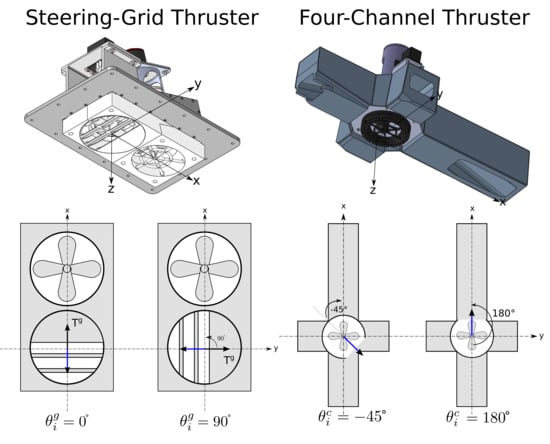
Therefore, in [7,8], they constructed a scale model of such a European class type I [9] self-propelled inland cargo barge. These self-propelled barges navigate with a non-conventional, over-actuated, fully-embedded actuation system configuration consisting of a 360-degrees-steerable steering-grid thruster in the bow in conjunction with a 360-degrees-steerable four-channel thruster in the stern. Conventionally, inland vessels tend to have one or more propellers, regularly ducted to protect them and to increase their performance, which are often placed in conjunction with multiple rudders to boost their manoeuvrability. Occasionally, the addition of an azimuth or bow thruster further improves their manoeuvrability [10,11]. In comparison, conventional marine vessels have propeller(s)–rudder(s) configurations positioned at the stern [12], and some marine vessels do carry more exotic propulsion systems such as transversal thrusters, azimuth thrusters, podded propellers, contra-rotating propellers, or even water jets for high speed vessels [13]. In addition, be aware that most small unmanned surface vehicles (USVs) also make use of propeller–rudder configurations [14]. However, some unmanned underwater vessels additionally utilise tunnel thrusters to increase their steering behaviour [15].

Within this aforementioned accumulation of more conventional actuation systems, the tunnel and azimuth thrusters seem to show the largest similarities with the thrusters of this study. The general design and performance of the tunnel thrusters are discussed in [16,17]. Whereas the authors in [18] review the different azimuth thruster designs, architectures, and working principles, the authors in [19] additionally review complementary thruster phenomena such as thruster–thruster or thruster–hull interactions, and the author in [20] published experimental data for an azimuth thruster during both static and dynamic operations. Unfortunately, the modelling literature for both systems is quite scarce. The existing research mostly uses the open-water propeller characteristics, as derived by [21], for its starting point on which additional flow phenomena can be added. For example, the authors in [22] built a mathematical manoeuvring model containing azimuth thrusters including thruster–thruster interactions. Similarly, the authors in [15] suggested a tunnel thruster model for an underwater vehicle exhibiting small yaw or pitch angles, and noted the scarcity of available models, probably due to the complexity of the flow phenomena at hand. Albeit certain parallels can be drawn between the actuation system in this study and these more conventional tunnel and azimuth systems, the usability and adequacy of these conventional modelling approaches need to be investigated. Therefore, this study aims to:

(i)

Detail the mechanical design of both the 360-degrees-steerable steering-grid thruster and the 360-degrees-steerable four-channel thruster nested inside the new fleet of ${\mathrm{Watertruck}}^{+}$ barges.

(ii)

Discuss, list, and show experimental towing tank data from both thrusters at different azimuth angles and propeller speeds, at zero advance speed.

(iii)

Investigate the adequacy of the open-water propeller characteristics as the kernel of the theoretical thrust modelling approach.

(iv)

Incorporate azimuth-angle-dependent internal and external hull thrust deduction losses by means of an extension to the theoretical model from (iii)

(v)

Offer an additional artificial neural network modelling approach that might be useful to grip the current, and perhaps future, inherent complex flow phenomena occurring within both thrusters.

The successful completion of these aims offers the future researcher three different thrust characteristic descriptions (i.e., a data table (ii), an extended physically-based model (iii)+(iv), and an artificial neural network (v)) for both actuation systems (i). In addition to the insights that these data descriptions provide, their information can also be leveraged by advanced motion controllers, thrust allocation algorithms, and plant models. This paper continues as follows: first, Section 2 shows the constructed vessel and details its non-conventional over-actuated propulsion system. Afterwards, Section 3 expands the theoretical thrust model with angle-dependent thrust deductions and explains the multilayer neural network model structures. Subsequently, Section 4 lists the experimental towing-tank data and feeds these data to both modelling methods. Finally, Section 5 provides a comparison and discussion of the modelling results, and Section 6 concludes this study.

2. Material

This section starts with a brief description of the overall design philosophy of the new fleet of self-propelled inland barges in Section 2.1. Afterwards, it details the mechanical design of both the steering-grid and the four-channel thruster in Section 2.2 and Section 2.3, respectively. Finally, it concludes with a detailed summary of the main differences between these thrusters and the more conventional actuation systems in Section 2.4.

2.1. Self-Propelled Inland Barges

During its first phase, the ${\mathrm{Watertruck}}^{+}$ project will construct 12 unpropelled barges, 16 self-propelled barges, and 3 push vessels of European Class type I–II. Their final deliverable aims towards building 500 vessels in the European Class range I–IV [6]. In order to gain insight in the automation potential of these vessels, and in order to study the technological feasibility, and current or future limitations, of unmanned inland cargo vessels, the authors constructed a scale model of a self-propelled barge of European Class type I. The real-size counterpart has a length of 38.5 m, a beam of 5.05 m, and a maximal draught of 2.8 m, whereas the KU Leuven scale model has a similar geometry, scaled down with a factor of 8. Figure 1a shows four real-size ${\mathrm{Watertruck}}^{+}$ barges of European Class type I, and one push vessel (slightly visible on the right), and (b) the KU Leuven scale model deployed as an unmanned, autonomous, inland cargo vessel. Figure 2a depicts a three-dimensional design drawing of this scale model where the embedded four-channel thruster (b), and steering-grid thruster (c) can be seen on the left-hand side and right-hand side of the vessel, respectively. This figure shows the vessel with open hatches in (a), which are the grey rectangular extensions on the top of the image, and sails with closed hatches in Figure 1b. As shown on Figure 2, the axes of the body-fixed reference frames which are used for all components throughout this paper point as follows: the x-axis towards the bow, y-axis towards starboard, and the z-axis towards the bottom. Both thrusters have a Kaplan Ka-series propeller without nozzle with a blade area ratio 0.65, and a pitch-diameter ratio of 0.95. The diameter of the steering-grid propeller measures 100 mm, whereas the diameter of the four-channel propeller measures 150 mm.

2.2. Mechanical Design Steering-Grid Thruster

The 360-degrees-steerable steering-grid bow thruster consists of two main parts: the propeller providing the thrust force, and the steering grid which orients the outflow of the water stream and thus provides the steering capabilities. Figure 3a shows a longitudinal cut of this thruster, i.e., along the $xz$-plane through the origin of Figure 2c. The propeller and its tilted shaft can be seen on the right side of the cut, where an anti-debris grid covers the inlet hole. The left-hand side shows the axis of the steering grid, but the grid itself is not shown to increase the image readability.

Figure 3b shows an abstract top view of the bottom section of this thruster which illustrates the chosen angle convention of the internal control angle of the steering grid, ${\theta }_i^g$. The drawn blue arrows show the orientation of the exiting water flow, which is opposite in direction compared to the thrust force, $T^g$. It is assumed that internal control angle, ${\theta }_i^g$, is equal to the output angle, ${\theta }_o^g$, of $T^g$, i.e., the flow exits the grid in alignment with the grid position in the $xy$-plane. Therefore, ${\theta }_i^g$ immediately gives the orientation of $T^g$. On top of that, the steering grid has a static angle, $\alpha$, of approximately 28° (curved surface), relative to the x-axis in the $xz$-plane, visible in Figure 2c. To illustrate this angle, the drawn blue arrows in Figure 3a show the exiting water flow in the $xz$-plane for ${\theta }_i^g={\theta }_o^g=0$° which can also be seen in in the $xy$-plane in Figure 3b on the left.

2.3. Mechanical Design Four-Channel Thruster

The 360-degrees-steerable four-channel stern thruster consists of two main parts: its propeller to induce thrust forces, and a 360-degrees-rotatable steering mechanism consisting of half a sphere with an opening of approximately 85° to orient its exiting water flow. Figure 4a shows a longitudinal section of this four-channel thruster, in the $xz$-plane in the origin of its body fixed reference frame. This section shows the propeller and its shaft together with the steering mechanism (of which only the bottom section is shown) which points towards the stern. This orientation would guide the exiting water flow towards the outlet channel on the left which points to the stern. The other shown outlet channel points to the bow, and the other two transversal outlet channels cannot be seen in this cut. Notice that the two shown outlets have a downwards angle of approximately 15° relative to the x-axis in the $xz$-plane, measured from the outlet of the internal steering mechanism—whereas the two transversal outlets have no downwards angle but are positioned a bit higher, directly in line of the internal outlet of the steering mechanism. This height–position difference of the outlets can be seen in Figure 2b.

Figure 4b depicts the angular convention of the internal control angle of the four-channel thruster ${\theta }_i^c$ which orients the theoretical outflow of the water stream, denoted by the blue arrows. Due to the geometric differences of the thruster channels, one cannot assume that ${\theta }_i^c$ will equal the output angle, ${\theta }_o^c$, of the resulting thrust force, $T^c$. The main geometric design effects that cause this discrepancy between ${\theta }_i^c$ and ${\theta }_o^c$ seem to be: (i) the fact that the water flow can only exit through one (e.g., Figure 4d at ${\theta }_i^c=180$°), or a superposition of two (e.g., Figure 4d at ${\theta }_i^c=-45$°) channels simultaneously, (ii) the different channel lengths and shapes (e.g., downwards bends), (iii) internal deflections of the water stream in the $xy$-plane when ${\theta }_i^c\ne$ 0°, 90°, 180°, or −90°, and (iv) a potentially remaining angular velocity of the water flow as there is no grid to align the outflow of the water. Therefore, in this study, the resulting four-channel thrust, $T^c$, will be orthogonally decomposed in its longitudinal, $T_x^c$, and transversal, $T_y^c$, components for different propeller speeds, $n^c$, according to:

$$T^c(n^c,{\theta }_i^c)=\sqrt{T_x^c{(n^c,{\theta }_i^c)}^2+T_y^c{(n^c,{\theta }_i^c)}^2},\hspace{1em}{\theta }_o^c=arctan\left(\frac{T_y^c}{T_x^c}\right).$$

(1)

2.4. Differences with Conventional Actuation Systems

In summary, the main design differences of both thrusters in this study compared to the more conventional thrusters appear to be the simultaneous occurrence of: (i) having the rotational axes of the propellers perpendicular (or almost perpendicular in case of the steering-grid) to the calm water plane, hence the propellers rotate in a plane parallel to the $xy$-plane, (ii) being completely nested inside the hull and thus not positioned directly in the ambient flow field, (iii) drawing in water from underneath the vessel hull, (iv) having both an inlet and an outlet positioned in the hull, not unlike jet systems, (v) having an internal deflection or rotation of the water stream from inlet to outlet, and (vi) having a 360-degrees-steerable outflow of the accelerated water provided by a steering mechanism, where the propeller itself does not change its position or orientation.

3. Modelling Structures and Identification Procedures

This study offers two different modelling approaches: one based on the open-water propeller characteristics, handled by Section 3.1, and one using artificial neural networks, explained by Section 3.2. Afterwards, Section 3.3 details the identification procedures for both modelling approaches.

3.1. Propeller Characteristics Thrust Model

This section uses the open-water propeller characteristics model of [21] as a starting point to construct new model structures. This open-water model takes a first order linearised lift force approximation of the propeller blades to calculate their theoretical thrust force. Given the fact that this lift force is a physical characteristic of the blade geometry, it is deemed suitable as a starting point to model both conventional and non-conventional actuation systems that use a propeller (for example, see its use for the tunnel and azimuth thrusters discussed in Section 1). Afterwards, this model will be expanded by adding the more complex flow phenomena that occur in the propulsion systems of this study. The model of [21] found the theoretical thrust force, $T_{th}$, to be quadratically dependent on the revolution speed of the propeller shaft, n, and bi-linearly dependent on the shaft speed and axial inflow velocity, $V_A$:

$$T_{th}=T_{nn}{n}^2+T_{n_{V_A}}n{V}_A.$$

(2)

It is common to introduce the non-dimensional thrust coefficient, $K_T$, and non-dimensional advance ratio, J, to express the ship propeller performance, by introducing:

$$K_T=\frac{T_{th}}{\rho n^2{D}_p^4},$$

(3)

$$J=\frac{V_A}{n{D}_p},$$

(4)

where $\rho$ is the water density and $D_p$ the propeller diameter. Moreover, for the conventional open-water propeller configurations, $K_T$ is often adequately approximated by a linear expression in J:

$$K_T=K_{T_0}+K_{T_J}J.$$

(5)

Combining Labels (2), (3), (4), and (5) gives:

$$T_{th}=K_{T_0}\rho D_p^4{n}^2+K_{T_J}\rho D_p^{3}n{V}_A,$$

(6)

which expresses the same information as Label (2) with:

$$T_{nn}=K_{T_0}\rho D_p^4,\hspace{1em}{T}_{nv}=K_{T_J}\rho D_p^3.$$

(7)

Furthermore, $V_A$ can be written as a fraction of the total speed of the vessel, U, by introducing the wake factor, w, which accounts for the speed reduction of the flow field at the inlet of the propeller:

$$V_A=(1-w)U.$$

(8)

In addition, the available thrust force for the vessel, T, is a fraction of the generated $T_{th}$ due to propeller–hull–interaction losses, accounted for by the thrust deduction number, t, which is assumed to be speed-independent:

$$T=(1-t)T_{th}.$$

(9)

In conclusion, by accumulating Labels (6), (8), and (9), T becomes:

$$T=(1-t)\left[K_{T_0}\rho D^4{n}^2+K_{T_J}\rho D^{3}n(1-w)U\right]=(1-t)\left[T_{nn}{n}^2+T_{n_{V_A}}n(1-w)U\right].$$

(10)

Note that (10) does not model the propeller dynamics, which can have a noticeable effect when manoeuvring at lower speeds [23]. Consequently, for some applications, it might be useful to extend T with these dynamics, as demonstrated in [24]. However, the experimental data of this study do not include transient dynamic measurements, and therefore their effects are omitted henceforth. Furthermore, as described in Section 4.1, the experiments were performed with zero advance speed, hence, $K_T=K_{T_0}$. Combining this information, (10) tailors further down to:

$$T=(1-t)T_{nn}{n}^2$$

(11)

for this study. The model complexity of the thrusters in this study, which is summarised by Section 2.4, lies mainly in the angle-dependent thrust deduction, i.e., making $t=f\left({\theta }_i\right)$. Moreover, both internal and external thrust deductions can occur as the water flows over the external hull, into the thruster inlet, and then through the nested thruster, and thus internal hull, itself, resulting in:

$$t=t_i+t_e=f\left({\theta }_i\right)=t_i\left({\theta }_i\right)+t_e\left({\theta }_i\right)=t\left({\theta }_i\right)$$

(12)

where $t_i$ and $t_e$ respectively indicate the internal and external hull-interaction thrust deductions. Hence, (11) refines to:

$$T=[1-t\left({\theta }_i\right)]T_{nn}{n}^2=\left(1-[t_i\left({\theta }_i\right)+t_e\left({\theta }_i\right)]\right)T_{nn}{n}^2.$$

(13)

Finally, in order to avoid a model structure bias in the identification results, the theoretical thrust force will be investigated and modelled as an unknown polynomial function in n, $T_{th}=f\left(n\right)=T_m\left(n\right)$. This approach does not force $T_{th}$ to equal $T_{nn}{n}^2$ when $U=0$. Accordingly, this method can thus validate whether the originally derived quadratic propeller-speed dependent thrust model indeed provides the best data fit. Ultimately, the thrust forces T to be identified according to the theoretic model in this study turn into:

$$T=[1-t\left({\theta }_i\right)]T_m\left(n\right).$$

(14)

3.2. Feedforward Multilayer Network Thrust Model

This section describes the architecture of feedforward multilayer neural networks that offer an alternative modelling approach to describe the complex flow phenomena discussed in this study. In general, artificial neural networks have one input layer, a number of hidden layers, and one output layer. However, a multilayer feedforward network with a non-polynomial activation function and only one hidden layer can already serve as a universal approximation for any nonlinear function [25]. This statement means that, regardless of the complexity of the flow phenomena that occur in our system, there will always exist network structures that can approximate the data sets. The capacity of these neural networks to model nonlinear characteristics drove the decision to add this alternative modelling approach.

In order to describe the general layout of a multilayer feedforward network, imagine the following example. If one takes an input vector, $x\in {\mathbb{R}}^m$, and an output vector, $y\in {\mathbb{R}}^l$, separated by one hidden layer with $n_h$ hidden neurons, and connects the hidden layer to y via $W\in {\mathbb{R}}^{l\times n_h}$ and to x via $V\in {\mathbb{R}}^{n_h\times m}$ with the addition of a bias vector, $\beta \in {\mathbb{R}}^{n_h}$, to the latter and an enveloping activation function, $\sigma (·)$, the following matrix–vector expression will describe the model structure:

$$y=W\sigma (Vx+\beta ),$$

(15)

which can also be expressed in an element-wise form, for i = 1, …, l, according to:

$$y_i=\sum _{r=1}^{n_h}{w}_{ir}\sigma (\sum _{j=1}^m{v}_{rj}{x}_j+{\beta }_r)$$

(16)

Figure 5 illustrates such a network hierarchy with the following model structure: two inputs (m = 2), one hidden layer of three neurons ($n_h=3$) of which the bias terms are not explicitly shown, two outputs (l = 2), and interconnection weights $w_{ij},v_{ij}$.

Be aware that these descriptions, (15) and (16), implicitly use a linear activation function for the output layer, although this is not necessary. Furthermore, the $\sigma (·)$ can have any shape, but typically a nonlinear function, such as sigmoid, tangent, hyperbolic tangent, etc., is used in order to exploit their characteristics when one trains the network with experimental data. Note that, similarly to (15), a second hidden layer could be inserted, resulting in:

$$y=W{\sigma }_2(V_2{\sigma }_1(V_{1}x+{\beta }_1)+{\beta }_2),$$

(17)

with $n_{h_1}$ and $n_{h_2}$ neurons in the hidden layers, connection-weight matrices, $W\in {\mathbb{R}}^{l\times n_{h_2}}$, $V_2\in {\mathbb{R}}^{n_{h_2}\times n_{h_1}}$, $V_1\in {\mathbb{R}}^{n_{h_1}\times m}$, bias vectors, ${\beta }_2\in {\mathbb{R}}^{n_{h_2}}$, ${\beta }_1\in {\mathbb{R}}^{n_{h_1}}$, and activation functions, ${\sigma }_1(·)$ and ${\sigma }_2(·)$. This hidden-layer insertion can be repeated to add multiple layers in an equivalent manner. The amount of hidden layers, their number of neurons, and the activation function types can all be chosen by the user. These design aspects offer great flexibility on the one hand, but an infinite amount of possible network architectures on the other hand. Accordingly, a few network designs will be shown in the results section which offers the possibility to compare their performance. These developed multilayer feedforward networks were trained to generate an output vector y (based on their input vector x), which aims to represent the desired output vector, i.e., the measured towing-tank data sets. More details of this network training procedure can be found in Section 3.3.2.

3.3. Model Identification Procedures

The theoretically derived thrust model of Section 3.1 and the neural networks of Section 3.2 provide a ${\theta }_i$-dependent and n-dependent model structure for the modelled thrust forces, $T(n,{\theta }_i)$, to which their respective experimental data sets, $D(n,{\theta }_i)$, can be fitted. Equation (18) shows the chosen cost function which calculates the least squares error, E, between the models and their data, i.e., between $T(n,{\theta }_i)$ and $D(n,{\theta }_i)$, for P data points. Section 3.3.1 and Section 3.3.2 explain the procedure to minimize (18), and thus maximize the model fit, for each afore-mentioned model structure of which the maximal model complexity was iteratively determined based on its impact on the final residuals:

$$E=\sum _{p=1}^P{\left(T(n_p,{\theta }_{i,p})-D(n_p,{\theta }_{i,p})\right)}^2$$

(18)

3.3.1. Identification Propeller Characteristics Model

The introduction of (14) into (18) produces the generic cost function for the model structures of Section 3.1:

$$E=\sum _{p=1}^P{\left([1-t\left({\theta }_{i,p}\right)]T_m\left(n_p\right)-D(n_p,{\theta }_{i,p})\right)}^2.$$

(19)

Within this study, the maximum polynomial orders for $t\left({\theta }_i\right)$ and $T_m\left(n\right)$ were respectively chosen to be quintic and cubic; hence, in this situation, E would equal:

$$E={\sum }_{p=1}^P{\left([1-(t_5{\theta }_{i,p}^5+t_4{\theta }_{i,p}^4+t_3{\theta }_{i,p}^3+t_2{\theta }_{i,p}^2+t_1{\theta }_{i,p}+t_0)](T_{nnn}{n}_p^3+T_{nn}{n}_p^2+T_n{n}_p)-D(n_p,{\theta }_{i,p})\right)}^2.$$

(20)

Furthermore, Section 4 also identifies the model structures of $T_m\left(n\right)=T_{nn}{n}^2$ or $T_{nnn}{n}^3$, given that the former aligns with the theoretical model of [21] (see Section 3.1), whereas for $t\left({\theta }_i\right)$ all coefficients of its polynomial model will be identified. A Python (version 3.6) script performed the minimization of (20) by using the least_squares() function from the open source SciPy packages [26]. This function determined its step size of the optimization problem, i.e., changing the values of the coefficients of $t\left({\theta }_i\right)$ and $T_m\left(n\right)$ in order to minimize (20), based on a trust region reflective method, based on the algorithm from [27].

3.3.2. Identification Feedforward Multilayer Network Model

The term feedforward refers to the calculation of y based on x, as these data run through the network of Figure 5 from left to right. Afterwards, the cost function (21) can be determined by the insertion of y from, for example (15) or (17), into (18):

$$E=\sum _{p=1}^P{\left(y_p-D(n_p,{\theta }_{i,p})\right)}^2,$$

(21)

where $y_p$ represents the network output of the p-th data point, which would be generated by the p-th input point, $x_p$. Within this study, the deepest developed network structure embodied two hidden layers; subsequently, its cost function can be defined by:

$$E=\sum _{p=1}^P{\left(W{\sigma }_2(V_2{\sigma }_1(V_1{x}_p+{\beta }_1)+{\beta }_2)-D(n_p,{\theta }_{i,p})\right)}^2.$$

(22)

Note that the p inputs for this network, $x_p$, are the same inputs as for the data points $D(n_p,{\theta }_{i,p})$; hence, (22) refines to:

$$E=\sum _{p=1}^P{\left(W{\sigma }_2(V_2{\sigma }_1(V_1(n_p,{\theta }_{i,p})+{\beta }_1)+{\beta }_2)-D(n_p,{\theta }_{i,p})\right)}^2.$$

(23)

Analogously to Section 3.3.1, this cost function (23) needs to decrease in order for the model fitness to increase. A common way to alter the distance between the data and the network is to use the back-propagation method as first suggested by [28]. This method derives an analytical expression of the gradient of the cost function for each neuron in the network by means of an iterative calculation from the right to the left in Figure 5, hence the name backpropagation, and uses this gradient to update the weights. Furthermore, one can augment this method by using the Levenberg–Marquardt algorithm to determine the updates of the connection weights [29]. This augmented back-propagation method was used in this study. Finally, in order to construct a network that generalises well to new inputs, one should avoid the over-fitting of data. Several regularisation methods exist to achieve this generalisation of the network. This study shows two regularisation methods: the early-stopping approach [30], and the Bayesian regularisation procedure of [31,32].

The early-stopping regulation divides x in a training, $x^t$, and a validation, $x^v$, set. Afterwards, it trains the network with the training data and tests the updated network with the validation data. When the error on the validation set, $E\left(x^v\right)$, starts to rise, although the error of the training data, $E\left(x^t\right)$, is still decreasing, the iterative algorithm stops, whereas, like the name suggests, Bayesian regulation uses the principles of the Bayesian probability theory as its regularisation principle. This regularisation is achieved by adding a term that penalises the size of weights, e.g., for a total of j weights w:

$$E_w=\sum _j{w}_j^2,$$

(24)

to the cost function (23). In addition, within this approach, the Bayesian probability theory automatically embeds Ocam’s razor principle by punishing too flexible and too complex module structures based on the Bayesian evidence principle [31]. Hence, this approach offers an automatic regularisation method, which boosts the generalisation of the trained networks. A collection of Matlab scripts constructed all the networks within this study. Consequently, the two afore-mentioned regularisation methods were applied by respectively calling the ‘trainlm’ [29], and ‘trainbr’ [33] function calls within the Matlab neural network environment. For the former, a data division of 70% training and 30% validation data was used. Note that this data separation is not necessary for the latter as it has an automatic regularisation approach as mentioned above.

4. Results

This section starts with listing and illustrating the raw experimental towing tank data from both thrusters in Section 4.1. Afterwards, Section 4.2 takes these data sets to identify the models described by (14) from Section 3.3.1, and similarly Section 4.3 trains the networks given by (15) and (17) from Section 3.3.2. All these results will be briefly discussed in each section, whereas an overall discussion and comparison between the results can be found in Section 5.

4.1. Experimental Towing-Tank Data

The experimental data for both thrusters were measured in a towing tank facility in deep water at zero advance speed, i.e., as a bollard pull test, and can be found in Section 4.1.1 for the steering-grid, and in Section 4.1.2 for the four-channel thruster.

4.1.1. Steering-Grid Thruster Data

The steering-grid thruster performed its bollard pull tests as a stand-alone device without enveloping ship hull hence only the internal angle-dependent hull losses occurred, i.e., $t=t_i=t_i\left({\theta }_i^g\right)$. In addition, given the assumption that ${\theta }_i^g={\theta }_o^g$, as mentioned in Section 2.2, the resulting thrust force data from the steering-grid thruster, $D^g$, were measured in alignment with the angle of the steering grid, using a planar beam load cell of the type LCPB series of OMEGA with a maximal error of 1%.

Table A1. Data steering-grid thruster $D^g(n^g,{\theta }_i)$ [N].

${\mathit{\theta }}_{\mathit{i}}$ [°]	500 rpm	1000 rpm	1500 rpm
0	1.85	7.47	13.70
30	2.30	8.08	15.16
60	1.75	7.64	15.30 1
90	1.64	6.68	14.52
120	1.79	6.57	13.11
150	0.81	3.41	7.79
180	0.79	3.36	8.12

¹ data point calculated based on Table A3b with a quadratic fit for $t\left(\theta \right)$.

in Appendix A summarises these different $D^g$ measurements at different ${\theta }_i^g$ and different rotational speeds of the propeller, $n^g$, i.e., $D^g=D^g(n^g,{\theta }_i^g)$. Subsequently, Figure 6 outlines these data points on a polar plot, assuming symmetry over the longitudinal x-axes. The decrease in thrust force for ${\theta }_i^g\in [150,180]$° might be explained by the potential occurrence of a recirculation zone of water flow, as in this orientation the exiting water stream is pointed towards the inlet of the steering-grid thruster.

4.1.2. Four-Channel Thruster Data

The bollard pull tests of the four-channel thruster were performed inside half a ship hull, which was split in the transversal direction, i.e., cut in the $yz$-plane at midship. Consequently, under the assumption that the most crucial external thrust deduction effects, $t_e$, will be captured by using half a ship hull, $t\left({\theta }_i^c\right)$ becomes the sum of $t_i\left({\theta }_i^c\right)$ and $t_e\left({\theta }_i^c\right)$. Given the information that for the four-channel thruster, ${\theta }_o^c\ne {\theta }_i^c$, as indicated in Section 2.3, the thrust forces were measured on both the longitudinal x-axis, $D_x^c(n^c,{\theta }_i^c)$, and transversal y-axis, $D_y^c(n^c,{\theta }_i^c)$, of the four-channel thruster for different ${\theta }_i^c$ and propeller speeds, $n^c$. Therefore, similar to $T^c$, the total resulting measured thrust force of the four-channel thruster, $D^c$, can be derived from:

$$D^c(n^c,{\theta }_i^c)=\sqrt{D_x^c{(n^c,{\theta }_i^c)}^2+D_y^c{(n^c,{\theta }_i^c)}^2},\hspace{1em}{\theta }_o^c=arctan\left(\frac{D_y^c}{D_x^c}\right).$$

(25)

Table A2. Towing tank measurements of the 360-degrees-steerable four-channel stern thruster.

${\mathit{\theta }}_{\mathit{i}}^{\mathit{c}}$ [°]	${\mathit{n}}^{\mathit{c}}$ [rpm]	${\mathit{D}}_{\mathit{x}}^{\mathit{c}}$ [N]	${\mathit{D}}_{\mathit{y}}^{\mathit{c}}$ [N]	${\mathit{D}}^{\mathit{c}}$ [N]	${\mathit{\theta }}_{\mathit{o}}^{\mathit{c}}$ [°]
0	354	6.98	0.10	6.98	0.82
−30	348	2.49	−3.09	3.97	−51.14
−45	328	1.71	−3.56	3.95	−64.34
−60	330	0.60	−5.62	5.65	−83.91
−90	325	0.37	−6.86	6.87	−86.91
−120	336	0.52	−4.63	4.66	−83.59
−135	337	−1.27	−2.27	2.60	−119.23
−150	334	−3.68	−0.13	3.68	−177.98
−180	360	−7.32	−0.22	7.32	−178.28
0	660	23.78	0.68	23.79	1.64
−30	653	7.85	−11.46	13.89	−55.59
−45	628	6.20	−12.72	14.15	−64.01
−60	626	2.01	−20.33	20.43	−84.35
−90	617	2.48	−26.15	26.27	−84.58
−120	630	2.22	−16.69	16.84	−82.42
−135	628	−4.82	−8.38	9.67	−119.91
−150	636	−13.15	−0.52	13.16	−177.74
−180	665	−24.91	−0.13	24.91	−179.70
0	960	51.06	1.26	51.08	1.41
−30	952	16.60	−24.50	29.59	−55.88
−45	930	13.23	−27.56	30.57	−64.36
−60	925	4.61	−45.45	45.68	−84.21
−90	925	4.83	−58.38	58.58	−85.27
−120	938	5.39	−36.35	36.75	−81.57
−135	935	−10.45	−18.30	21.07	−119.73
−150	934	−29.63	−1.44	29.66	−177.22
−180	966	−53.43	−1.06	53.44	−178.86
0	1255	87.64	1.99	87.66	1.30
−30	1248	28.34	−42.07	50.73	−56.03
−45	1219	23.00	−47.14	52.45	−63.99
−60	1216	7.72	−79.07	79.45	−84.42
−90	1215	8.45	−102.88	103.23	−85.30
−120	1226	9.23	−64.20	64.86	−81.82
−135	1226	−18.17	−32.13	36.91	−119.49
−150	1226	−51.58	−2.57	51.64	−177.15
−180	1260	−92.01	−2.24	92.04	−178.61
0	1545	134.40	3.36	134.44	1.43
−30	1538	43.05	−64.44	77.50	−56.25
−45	1515	35.41	−72.83	80.98	−64.07
−60	1510	11.36	−121.99	122.52	−84.68
−90	1510	10.80	−160.79	161.15	−86.16
−120	1515	13.26	−99.74	100.62	−82.43
−135	1515	−28.21	−49.33	56.83	−119.76
−150	1515	−79.17	−5.21	79.34	−176.23
−180	1550	−140.19	−4.15	140.25	−178.30

in Appendix B lists all the four-channel thruster data points, measured by a UDW3 force/torque sensor from AMTI, with a maximal error of 3% per component (mainly due to the possibility of cross-talk). Thereupon, Figure 7 illustrates these measurements in two different perspectives. Firstly, plot Figure 7a,b show the decomposed measured thrust forces for ${\theta }_i^c\in [0,-180]$° at different $n^c$. Note that the small fluctuations in $n^c$, reported in Table A2, are accumulated around their mean value in order to plot these data sets with one line, resulting in for example: $n^c=340\pm 25$ rpm. Secondly, plot Figure 7c,d shows exactly the same data as plot Figure 7a,b, but transformed into ${\theta }_o^c$ and $D^c$, calculated according to (25).

Figure 7c confirms the nonlinear mapping of ${\theta }_i^c$ to ${\theta }_o^c$ hypothesis, which appeared to stay consistent over different $n^c$-sets. This $n^c$-independent consistency in the angle mapping seems to hint at a structural, geometrical origin of this nonlinearity. The relatively constant ${\theta }_o^c$ for ${\theta }_i^c\in$ [−60°, −120°] seems to originate from the incapability of the thruster to produce a significant longitudinal force, i.e., $D_x^c$, within this angular domain allowing the transversal force $D_y^c$ to dominate the thrust generation, which results in an almost transversal ${\theta }_o^c$. The inverse seems to be true for ${\theta }_o^c$ when ${\theta }_i^c\in$ [−150°, −180°]. Given the currently available data sets, it remains hard to judge the explicit cause of these nonlinearities. However, Section 2.3 ended with a list of possible contributors to this nonlinear mapping.

4.2. Identification of the Propeller-Characteristics-Based Thrust Models

Plugging the data sets from Section 4.1 into the cost function of (20) allows for the identification of the modelled thrust forces according to (14). By varying the order of the polynomials of $t\left(\theta \right)$ and $T_m\left(n\right)$ up to their respective maximums of quintic and cubic, one can compare the resulting model complexities based on the residuals of their cost functions. This comparison offers a bias-variance trade-off during the eventual model selection [34]. The final model selection depends on the requirements of its end user. Section 4.2.1 calculates $T^g(n^g,{\theta }_i^g)$ by using $D^g(n^g,{\theta }_i^g)$, whereas Section 4.2.2 calculates the orthogonal decomposition of $T^c(n^c,{\theta }_i^c)$ into $T_x^c(n^c,{\theta }_i^c)$ and $T_y^c(n^c,{\theta }_i^c)$ by respectively using $D_x^c(n^c,{\theta }_i^c)$ and $D_y^c(n^c,{\theta }_i^c)$.

4.2.1. Steering-Grid Thruster Identification Propeller-Characteristics-Based Thrust Models

Due to the absence of the hull in the towing-tank experiments of Section 4.1.1, no external hull thrust deductions occurred (except for the small external surface of the thruster itself which will be neglected here), i.e., $t\left({\theta }_i^g\right)=t_i\left({\theta }_i^g\right)$. This paves the way to identify $t_e\left({\theta }_i\right)$ by the future increase in thrust deduction when the actuation sits inside its hull by using: $t\left({\theta }_i\right)=t_i\left({\theta }_i\right)+t_e\left({\theta }_i\right)$.

Table 1. Cost function residuals for the different $T^g$ models.

Model $\mathit{t}\left({\mathit{\theta }}_{\mathit{i}}^{\mathit{g}}\right)$	${\mathit{T}}_{\mathit{nnn}},{\mathit{T}}_{\mathit{nn}},{\mathit{T}}_{\mathit{n}}$	${\mathit{T}}_{\mathit{nn}},{\mathit{T}}_{\mathit{n}}$	${\mathit{T}}_{\mathit{nnn}}$	${\mathit{T}}_{\mathit{nn}}$	${\mathit{T}}_{\mathit{n}}$
Constant	39.26	39.83	64.79	41.24	62.12
Linear	12.77	13.35	39.85	14.84	37.01
Quadratic	5.67	6.12	31.72	7.28	31.88
Cubic	4.11	4.47	29.10	5.38	31.44
Quartic	2.62	2.96	27.32	3.80	30.39
Quintic	0.99	1.50	27.15	2.76	25.45

summarises the residuals of the cost functions after performing the afore-mentioned model fits. The absolute value of these residuals has no meaning; however, their relative size does as it indicates the relative model fitness of the underlying model structure. The columns denote the different model structures of $T_m\left(n^g\right)$, whereas the rows show the different polynomial orders of $t\left({\theta }_i^g\right)$. For example, a cubic-order model for $t\left({\theta }_i^g\right)$ in combination with $T_m\left(n^g\right)=T_{nn}{n}^{g^2}$ can be identified by:

$$E=\sum _{p=1}^P{\left([1-(t_3{\theta }_{i,p}^{g^3}+t_2{\theta }_{i,p}^{g^2}+t_1{\theta }_{i,p}^g+t_0)](T_{nn}{n}_p^{g^2})-D(n_p^g,{\theta }_{i,p}^g)\right)}^2.$$

(26)

Here, as visible in Table 1, the final cost of E would equal 5.38. To further clarify this representation of the results,

Table A3. Identified thrust model coefficients of Table 1.

					(a)
Order t($\mathit{\theta }$)	Cost	${\mathit{t}}_{\mathbf{5}}$	${\mathit{t}}_{\mathbf{4}}$	${\mathit{t}}_{\mathbf{3}}$	${\mathit{t}}_{\mathbf{2}}$	${\mathit{t}}_{\mathbf{1}}$	${\mathit{t}}_{\mathbf{0}}$	${\mathit{T}}_{\mathit{n}}$
Quintic	25.45	$3.68\times {10}^{-10}$	$1.61\times {10}^{-07}$	$-2.43\times {10}^{-05}$	$1.48\times {10}^{-03}$	$-2.98\times {10}^{-02}$	$1.33\times {10}^{-02}$	$8.40\times {10}^{-03}$
Quartic	30.39	0	$-5.25\times {10}^{-09}$	$1.72\times {10}^{-06}$	$-1.39\times {10}^{-04}$	$2.36\times {10}^{-03}$	$1.69\times {10}^{-02}$	$8.57\times {10}^{-03}$
Cubic	31.44	0	0	$-1.67\times {10}^{-07}$	$7.23\times {10}^{-05}$	$-4.87\times {10}^{-03}$	$-7.75\times {10}^{-03}$	$8.18\times {10}^{-03}$
Quadratic	31.88	0	0	0	$2.61\times {10}^{-05}$	$-1.72\times {10}^{-03}$	$-1.94\times {10}^{-02}$	$8.29\times {10}^{-03}$
Linear	37.01	0	0	0	0	$2.58\times {10}^{-03}$	$4.81\times {10}^{-03}$	$9.36\times {10}^{-03}$
Constant	62.12	0	0	0	0	0	$2.14\times {10}^{-02}$	$7.22\times {10}^{-03}$
					(b)
Order t($\mathit{\theta }$)	Cost	${\mathit{t}}_{\mathbf{5}}$	${\mathit{t}}_{\mathbf{4}}$	${\mathit{t}}_{\mathbf{3}}$	${\mathit{t}}_{\mathbf{2}}$	${\mathit{t}}_{\mathbf{1}}$	${\mathit{t}}_{\mathbf{0}}$	${\mathit{T}}_{\mathit{nn}}$
Quintic	2.76	$-1.86\times {10}^{-10}$	$7.75\times {10}^{-08}$	$-1.11\times {10}^{-05}$	$6.85\times {10}^{-04}$	$-1.63\times {10}^{-02}$	$7.76\times {10}^{-03}$	$6.37\times {10}^{-06}$
Quartic	3.80	0	$-6.58\times {10}^{-09}$	$2.01\times {10}^{-06}$	$-1.32\times {10}^{-04}$	$-5.03\times {10}^{-04}$	$8.35\times {10}^{-04}$	$6.36\times {10}^{-06}$
Cubic	5.38	0	0	$-3.52\times {10}^{-07}$	$1.30\times {10}^{-04}$	$-9.39\times {10}^{-03}$	$5.85\times {10}^{-03}$	$6.23\times {10}^{-06}$
Quadratic	7.28	0	0	0	$3.06\times {10}^{-05}$	$-2.55\times {10}^{-03}$	$8.08\times {10}^{-03}$	$6.57\times {10}^{-06}$
Linear	14.84	0	0	0	0	$2.60\times {10}^{-03}$	$-6.83\times {10}^{-03}$	$7.24\times {10}^{-06}$
Constant	41.24	0	0	0	0	0	$7.35\times {10}^{-06}$	$5.52\times {10}^{-06}$
					(c)
Order t($\mathit{\theta }$)	Cost	${\mathit{t}}_{\mathbf{5}}$	${\mathit{t}}_{\mathbf{4}}$	${\mathit{t}}_{\mathbf{3}}$	${\mathit{t}}_{\mathbf{2}}$	${\mathit{t}}_{\mathbf{1}}$	${\mathit{t}}_{\mathbf{0}}$	${\mathit{T}}_{\mathit{nnn}}$
Quintic	27.15	$-8.28\times {10}^{-11}$	$3.04\times {10}^{-}08$	$-3.75\times {10}^{-06}$	$2.34\times {10}^{-04}$	$-8.61\times {10}^{-03}$	$1.52\times {10}^{-02}$	$4.40\times {10}^{-09}$
Quartic	27.32	0	$-7.20\times {10}^{-09}$	$2.15\times {10}^{-06}$	$-1.31\times {10}^{-04}$	$-1.74\times {10}^{-03}$	$-9.32\times {10}^{-04}$	$4.34\times {10}^{-09}$
Cubic	29.10	0	0	$-4.42\times {10}^{-07}$	$1.58\times {10}^{-04}$	$-1.17\times {10}^{-02}$	$-1.29\times {10}^{-02}$	$4.17\times {10}^{-09}$
Quadratic	31.72	0	0	0	$3.30\times {10}^{-05}$	$-2.95\times {10}^{-03}$	$-3.40\times {10}^{-03}$	$4.48\times {10}^{-09}$
Linear	39.85	0	0	0	0	$2.56\times {10}^{-03}$	$-4.04\times {10}^{-03}$	$5.03\times {10}^{-09}$
Constant	64.79	0	0	0	0	0	$2.24\times {10}^{-08}$	$3.83\times {10}^{-09}$
					(d)
Order t($\mathbf{\theta }$)	Cost	${\mathit{t}}_{\mathbf{5}}$	${\mathit{t}}_{\mathbf{4}}$	${\mathit{t}}_{\mathbf{3}}$	${\mathit{t}}_{\mathbf{2}}$	${\mathit{t}}_{\mathbf{1}}$	${\mathit{t}}_{\mathbf{0}}$	${\mathit{T}}_{\mathit{nn}}$	${\mathit{T}}_{\mathit{n}}$
Quintic	1.50	$-2.00\times {10}^{-10}$	$8.44\times {10}^{-08}$	$-1.23\times {10}^{-05}$	$7.56\times {10}^{-04}$	$-1.71\times {10}^{-02}$	$9.49\times {10}^{-02}$	$5.74\times {10}^{-06}$	$1.70\times {10}^{-03}$
Quartic	2.96	0	$-6.65\times {10}^{-09}$	$2.05\times {10}^{-06}$	$-1.38\times {10}^{-04}$	$-1.56\times {10}^{-04}$	$-3.61\times {10}^{-02}$	$5.28\times {10}^{-06}$	$1.19\times {10}^{-03}$
Cubic	4.47	0	0	$-3.41\times {10}^{-07}$	$1.27\times {10}^{-04}$	$-9.15\times {10}^{-03}$	$-3.46\times {10}^{-02}$	$5.11\times {10}^{-06}$	$1.21\times {10}^{-03}$
Quadratic	6.12	0	0	0	$3.43\times {10}^{-05}$	$-2.78\times {10}^{-03}$	$-1.36\times {10}^{-01}$	$4.78\times {10}^{-06}$	$1.31\times {10}^{-03}$
Linear	13.35	0	0	0	0	$2.58\times {10}^{-03}$	$3.29\times {10}^{-04}$	$5.87\times {10}^{-06}$	$1.91\times {10}^{-03}$
Constant	39.83	0	0	0	0	0	$-7.91\times {10}^{-02}$	$4.11\times {10}^{-06}$	$1.35\times {10}^{-03}$
Order t($\mathbf{\theta }$)	Cost	${\mathit{t}}_{\mathbf{5}}$	${\mathit{t}}_{\mathbf{4}}$	${\mathit{t}}_{\mathbf{3}}$	${\mathit{t}}_{\mathbf{2}}$	${\mathit{t}}_{\mathbf{1}}$	${\mathit{t}}_{\mathbf{0}}$	${\mathit{T}}_{\mathit{nnn}}$	${\mathit{T}}_{\mathit{nn}}$	${\mathit{T}}_{\mathit{n}}$
Quintic	0.99	$-2.43\times {10}^{-10}$	$1.03\times {10}^{-07}$	$-1.51\times {10}^{-05}$	$9.27\times {10}^{-04}$	$-2.06\times {10}^{-02}$	$-4.62\times {10}^{-02}$	$-2.34\times {10}^{-09}$	$1.01\times {10}^{-05}$	$-1.05\times {10}^{-03}$
Quartic	2.62	0	$-9.61\times {10}^{-09}$	$2.97\times {10}^{-06}$	$-2.02\times {10}^{-04}$	$2.27\times {10}^{-05}$	$-5.09\times {10}^{-01}$	$-1.31\times {10}^{-09}$	$6.50\times {10}^{-06}$	$-5.91\times {10}^{-04}$
Cubic	4.11	0	0	$-3.32\times {10}^{-07}$	$1.24\times {10}^{-04}$	$-8.93\times {10}^{-03}$	$-3.87\times {10}^{-02}$	$-1.91\times {10}^{-09}$	$9.31\times {10}^{-06}$	$-8.55\times {10}^{-04}$
Quadratic	5.67	0	0	0	$5.45\times {10}^{-05}$	$-4.38\times {10}^{-03}$	$-8.26\times {10}^{-01}$	$-1.29\times {10}^{-09}$	$5.82\times {10}^{-06}$	$-5.85\times {10}^{-04}$
Linear	12.77	0	0	0	0	$2.51\times {10}^{-03}$	$2.83\times {10}^{-02}$	$-3.14\times {10}^{-09}$	$1.30\times {10}^{-05}$	$-1.44e-03$
Constant	39.26	0	0	0	0	0	$1.44\times {10}^{-01}$	$-2.75\times {10}^{-09}$	$1.13\times {10}^{-05}$	$-1.29\times {10}^{-03}$

in Appendix C lists all the identified model coefficients for all the model structures of Table 1. This information sheds more light on the cost residuals; for example, Table A3e shows negative values for $T_{nnn}$ which would mean a thrust deduction with increasing $n^g$, hence here the data seem to be over-fitted and thus losing physical meaning. Table 1 also seems to validate that taking $T_m\left(n\right)=T_{nn}{n}^2$ generates a simple but robust model which also aligns with the theoretically derived propeller-characteristics model of Section 3.1, as adding a linear propeller-speed dependency, $T_n$, to $T_m\left(n\right)$ results in marginally lower residuals. Nevertheless, this linear term could be added if desired.

Given the adequacy of $T_m\left(n\right)=T_{nn}{n}^2$, Figure 8a plots the identified quadratic, linear, and constant models for $t\left({\theta }_i^g\right)$ with $T_m\left(n\right)=T_{nn}{n}^2$, together with the data points $D^g(n^g,{\theta }_i^g)$ to illustrate the model fits. In addition, given the rather constant thrust decrease for ${\theta }_i^g\in [150,180]$°, one could also perform the above-mentioned modelling procedure of $T^g$ only for the ${\theta }_i^g\in [0,150]$° domain, and assume $T^g(n^g,{\theta }_i^g)=T^g(n^g,150$°) to be a constant value for ${\theta }_i^g\in [150,180]$°. Figure 8b illustrates this second methodology for $T^g$, using a quadratic fit for $t\left({\theta }_i^g\right)$. Figure 9 provides another way to visualise these models fits by plotting $T^g$ over its $n^g$ domain for ${\theta }_i^g=$ 0°, 90°, and 180° by using a quadratic model fit for $t\left({\theta }_i^g\right)$ and $T_m\left(n\right)=T_{nn}{n}^2$ for the aforementioned full ${\theta }_i^g$-domain fit in (a), and for the fit incorporating the constant thrust zone in (b). The latter plot, Figure 9b, shows the benefit of adding the constant thrust zone as it provides a better fit for ${\theta }_i^g=180$° compared to Figure 9a.

4.2.2. Four-Channel Thruster Identification Propeller-Characteristics-Based Thrust Models

The four-channel thruster generated its data sets embedded inside half a hull, making it impossible to diversify between $t_i\left({\theta }_i^c\right)$ and $t_e\left({\theta }_i^c\right)$ as they both depend on the same angle. Thus, this section identifies the thrust deduction coefficients as a superposition of both external and internal hull losses. Note that future towing-tank experiments without a hull, as have been done for the steering-grid thruster, could identify $t_i$ separately and thus also give $t_e$.

Table 2. Cost function residuals for the different $T^c$ models: (a) $T_x^c$, and (b) $T_y^c$.

(a)
Model$\mathit{t}\left({\mathit{\theta }}_{\mathit{i}}^{\mathit{c}}\right)$	${\mathit{T}}_{\mathit{n}}$	${\mathit{T}}_{\mathit{nn}}$	${\mathit{T}}_{\mathit{nnn}}$	${\mathit{T}}_{\mathit{nn}},{\mathit{T}}_{\mathit{n}}$	${\mathit{T}}_{\mathit{nnn}},{\mathit{T}}_{\mathit{nn}},{\mathit{T}}_{\mathit{n}}$
Constant	38,795.76	38,795.95	38,796.08	38,795.43	38,795.34
Linear	7292.64	5092.89	5719.02	5085.50	5074.75
Quadratic	7066.95	4860.48	5500.83	4853.59	4843.96
Cubic	3511.66	1267.95	2168.83	1267.48	1267.44
Quartic	3035.18	738.33	1630.70	737.48	737.46
Quintic	2644.39	313.48	1207.49	312.45	312.37
(b)
Model$\mathit{t}\left({\mathit{\theta }}_{\mathit{i}}^{\mathit{c}}\right)$	${\mathit{T}}_{\mathit{n}}$	${\mathit{T}}_{\mathit{nn}}$	${\mathit{T}}_{\mathit{nnn}}$	${\mathit{T}}_{\mathit{nn}},{\mathit{T}}_{\mathit{n}}$	${\mathit{T}}_{\mathit{nnn}},{\mathit{T}}_{\mathit{nn}},{\mathit{T}}_{\mathit{n}}$
Constant	22,722.75	21,261.84	22,199.03	21,255.83	21,223.65
Linear	22,173.90	20,707.77	21,684.97	20,700.10	20,662.85
Quadratic	7808.53	5129.44	6204.61	5128.91	5128.64
Cubic	6888.01	4515.32	5245.35	4144.76	4144.50
Quartic	3620.45	562.71	1654.30	559.84	559.09
Quintic	3414.50	356.56	1462.72	354.04	353.52

lists the different residuals of the cost functions of the model fitting algorithm for both $T_x^c$ in (a), and $T_y^c$ in (b). This table also gives the impression that $T_m\left(n\right)=T_{nn}{n}^2$ forms a simple and robust model structure to represent the theoretical thrust force, which again aligns with the theoretical derivation of Section 3.1. Here, too, adding $T_n$ (or $T_n$ and $T_{nnn}$) only generates marginal improvements compared to the quadratic $n^c$-dependency. Furthermore, this table indicates that the polynomial order of $t\left({\theta }_i^c\right)$ is better modelled by an odd function for $T_x^c$ and by an even function for $T_y^c$.

Figure 10 illustrates the model fits of $T_x^c$ in (a), and $T_y^c$ in (b) for different polynomial orders of $t\left({\theta }_i^c\right)$ with $T_m\left(n\right)=T_{nn}{n}^2$. Moreover, this figure also confirms the better fitness of odd $t\left({\theta }_i^c\right)$ functions for $T_x^c$ and even functions for $T_y^c$.

Given the above-mentioned rather constant thrust output of $D_x^c$ for ${\theta }_i^c\in$ [−60°, −120°], and of $D_y^c$ for ${\theta }_i^c\in$ [−150°, −180°], one could model these regions by a constant value. Subsequently, Figure 11a shows a piecewise linear model consisting of a linear fit of $T_x^c$ for ${\theta }_i^c\in$ [0°, −60°], a constant thrust zone where $T_x^c=T_x^c(-60$°) for ${\theta }_i^c\in$ [−60°, −120°], and finally again a linear fit for ${\theta }_i^c\in$ [−120°, −180°], whereas, similarly to Figure 10b, Figure 11b depicts a quartic and quadratic fit of $t\left({\theta }_i^c\right)$ for this angle in the [0°, −150°] domain followed by a constant thrust zone where $T_y^c=T_y^c(-150$°). As can be seen, this constant thrust zone offers a better representation of the data compared to the non-physical polynomial over fitting of Figure 10b on the same angular domain.

4.3. Identification of the Feedforward Multilayer Network Thrust Models

Similarly to Section 4.2, this section plugged the data from Section 4.1 into different feedforward multilayer network designs. Within the subsequent figures and tables, the abbreviations ‘br’, and ‘es’ respectively denote a Bayesian regulation and early stopping regulation scheme. These abbreviations will be followed by two numbers which indicate the amount of neurons in each hidden layer (e.g., br5-0, will only have one hidden layer with five neurons, whereas br3-3 would have two hidden layers with three neurons each). Furthermore, all networks used a tan–sigmoid transfer function, $tansig(·)$, for the activation functions of the hidden layers, i.e., $\sigma (·)=tansig(·)$. Finally, note that all the training procedures of the artificial neural networks within this study were initialised with random weights for the network coefficients. This random initialisation can have an impact on the final results. Therefore, all networks were trained five times and the subsequent tables will show the average, minimum, and maximum final residual cost for each network structure over all five of these training cycles. Analogously to Section 4.2, the model structures can be selected based on a bias-variance trade-off which depends on the requirements of the end user.

4.3.1. Steering-Grid Thruster Identification Multilayer Networks

The networks for the steering-grid thruster used $n^g$ and ${\theta }_i^g$ for the input vector, x, as these inputs also generated the experimental data, i.e., $D^g(n^g,{\theta }_i^g)$. The output vector of these networks, y, had only one element which constitutes the modelled thrust force, i.e., $y=T^g$. To exemplify the cost function calculation and consequently the identification of its neural network, (27) calculates the residual for a network which models the steering grid with one hidden layer of three neurons by plugging (16) into (21), and thus by minimising:

$$E=\sum _{p=1}^P{\left(\sum _{r=1}^3{w}_r\sigma (\sum _{j=1}^2{v}_{rj}{x}_{j,p}+{\beta }_r)-D(n_p^g,{\theta }_{i,p}^g)\right)}^2,$$

(27)

with $n_h=3$, $m=2$, and $l=1$ and thus its index is omitted. Accordingly, in matrix notation $W\in {\mathbb{R}}^{1\times 3}$, $V\in {\mathbb{R}}^{3\times 2}$, and $\beta \in {\mathbb{R}}^{3\times 1}$. The two input vector elements, i.e., $x_{1,p}$ and $x_{2,p}$ are $n_p^g$ and ${\theta }_{i,p}^g$, note that the subscript i from the latter refers to the internal actuation angle and not to an element notation. Depending on the selected training method, (27) can calculate the residual for es-3-0 or br-3-0, shown in

Table 3. Residuals cost functions of the multilayer feedforward neural networks for Figure 12: (a) one hidden layer, (b) two hidden layers.

(a)
Model	Average	Minimum	Maximum
es5-0	37.91	12.86	71.26
es3-0	22.82	12.86	51.23
es2-0	22.66	8.33	52.80
br5-0	7.63	7.62	7.63
br3-0	8.38	8.37	8.38
br2-0	10.60	10.60	10.60
(b)
Model	Average	Minimum	Maximum
es3-2	58.54	4.16	192.96
es3-1	80.16	4.16	235.70
br3-2	0.42	0.42	0.42
br3-1	0.37	0.37	0.37
br2-1	8.44	8.44	8.44

which lists the residuals of the final cost functions for all the identified network structures. Figure 12a plots the identification results of three different network topologies which only used one hidden layer which had two, three, or five neurons. Moreover, this figure compares the early stopping and Bayesian regulation approaches. Based on this plot, the Bayesian regulation outperformed the early stopping regulation. This performance difference can also be seen in Table 3a. In addition, Figure 12b shows similar identification results for two different network architectures which nested two hidden layers. Here too, one can observe the Bayes regulation method outperforming the early stopping approach, on which Table 3b provides further detail.

4.3.2. Four-Channel Thruster Identification Multilayer Networks

This section constructs different networks with two hidden layers and a Bayesian regulation approach for the four-channel thruster data. These specific network architectures were chosen based on their performance in the results of the steering-grid thruster, handled in Section 4.3.1. Although all the developed networks used $n^c$ and ${\theta }_i^c$ as their input values, three different approaches for the output, y, were selected to illustrate the network-architecture flexibility:

(i)

Fitting the orthogonally decomposed thrust forces separately, i.e., constructing two networks with one output each: one for deriving $T_x^c$ based on $D_x^c$, and analogously one for finding $T_y^c$ based on $D_y^c$.

(ii)

Fitting the orthogonally decomposed thrust forces simultaneously, i.e., constructing one network with two outputs, $T_x^c$ and $T_y^c$.

(iii)

Fitting the resulting thrust force and its orientation simultaneously, i.e., construction one network with two outputs, $T^c$ and ${\theta }_o^c$.

Table 4. Comparison of the identification residuals: (a) for the networks of (i) that model $T_x^c$, (b) for the networks of (i) that model $T_y^c$, (c) for the networks of case (ii), and (d) for the networks of case (iii).

(a)
Model	Average Cost	Minimum	Maximum
br2-2	17,390.56	2338.70	77,598.00
br3-2	962.83	292.15	1130.50
br3-3	253.10	220.82	301.59
br4-2	31,144.55	211.31	77,597.00
br4-3	192.64	192.64	192.64
br4-4	89.83	28.53	181.78
(b)
Model	Average Cost	Minimum	Maximum
br2-2	13,528.72	1252.90	62,631.00
br3-2	13,081.49	693.36	62,634.00
br3-3	299.16	114.91	636.50
br4-2	581.44	521.76	624.52
br4-3	388.45	4.24	518.54
br4-4	194.91	0.42	486.64
(c)
Model	Average Cost	Minimum	Maximum
br3-4	703.25	32.14	1279.90
br3-5	299.07	33.31	695.43
br5-3	587.82	558.14	657.58
br4-4	336.92	26.42	575.19
br5-3	587.82	558.14	657.58
br5-4	16.85	3.73	67.21
(d)
Model	Average Cost	Minimum	Maximum
br3-4	719.98	585.92	1256.20
br3-5	345.46	116.16	500.89
br5-3	27,349.43	748.15	34,017.00
br4-4	408.67	88.74	513.91
br5-3	27,349.43	748.15	34,017.00
br5-4	33,841.00	33,810.00	33,863.00

compares the final cost function residuals of different network topologies for these three different cases. Firstly, regarding case (i), (a) summarises the residuals for $T_x^c$ and (b) for $T_y^c$. Secondly, concerning case (ii), (c) shows the residuals of the chosen different network architectures to model this network which has two outputs. Thirdly, for case (iii), (d) shows a variety of model structures that represented this dual-output network. In addition, Figure 13 illustrates the fitness of several identified models for cases (i) to (iii). To plot these identified network structures, one of the five runs of the respective network designs was chosen at random. When one compares case (i) to case (ii), hence comparing the plots (a), (b) with (c), (d), the former seem to have less variance compared to the latter. However, caution should be taken when one compares these plots as they represent different network topologies, have different amounts of neurons and they are a random selection of one of the five network training cycles performed on each design.

5. Discussion

The pure experimental data of Section 4.1 already expose interesting results for both thruster designs. On the one hand, they show the potential occurrence of a recirculation zone of flowing water for certain positions of the steering grid. On the other hand, they highlight the rather biased output angles of the resulting thrust forces of the four-channel thruster. Nevertheless, additional experiments (e.g., setups with different channel geometries and lengths, propeller diameters, steering-mechanism designs, etc.) could provide complementary insights in the complex flow phenomena arising in these thrusters. In addition, experiments with $U\ne 0$ could identify the wake factor which might depend on both the vessel velocity and the thruster location, i.e., $w=f(U,X_t,Y_t,Z_t)$. Similarly, these experiments could further investigate the adequacy of (5) for these non-conventional thrusters. Note that the ambient flow, when $U\ne 0$, does not decrease the thruster performance, but the complex interactions between the water outlet and the surrounding flow can decrease the effective thrust [35]. Furthermore, experiments with dynamic propeller speeds could verify the adequacy of the existing dynamic thrust models, e.g., [24]. Here, one should note that the ambient flow field tends to not have a large impact on the propulsion system dynamics [36].

Given the complexity of the flow phenomena at hand, this study offered two model structure methodologies. Firstly, Section 4.2 validated the theoretical propeller-characteristics thrust model structures of Section 3.1 for both thruster designs by means of a bias-variance trade-off. This trade-off indicates that the quadratic propeller speed dependency indeed forms a simple but generic description of the resulting thrust forces for both embedded thruster designs at zero advance speed, although more complex model structures could be selected if desired by the end user. Moreover, Section 4.2 further illustrated the successful modelling approach to capture the internal control-angle dependent thrust deductions that exist in both propulsion systems. Evidently, the aforementioned additional experimental setups could also help to further refine the propeller-characteristics based thrust model with the above-discussed possible extensions to this model. Secondly, Section 4.3 demonstrated the possibility to use the multilayer feedforward networks from Section 3.2 to grasp the complex water flows. Bearing in mind that these networks can serve as universal approximations of nonlinear functions, they offer the capability to model more complex flow phenomena that might occur during future experiments with dynamic propeller speeds or when $U\ne 0$.

Figure 14 compares both model structure methodologies for the thrust forces generated by the four-channel thruster. Figure 14a depicts the longitudinal modelled forces, $T_x^s$, whereas (b) shows the transversal modelled forces, $T_y^s$. For $T_x^s$, a quintic model describes $t\left({\theta }_i^s\right)$ in conjunction with $T_m\left(n\right)=T_{nn}{n}^2$ for the propeller characteristics-based model, whereas a Bayesian regulated network of two hidden layers, with three neurons each, forms the neural network structure. A similar approach describes the structures of $T_y^s$, only here $t\left({\theta }_i^s\right)$ has a quartic order. In both cases, i.e., (a) and (b), the neural networks seem to outperform the theoretically based models. Particularly in (b), the theoretical model generates a non-physical fit for ${\theta }_i^c\in$ [−150°, −180°] whereas the neural network does not. In (a), for ${\theta }_i^c\in$ [−60°, −120°] at $n^c=1530$ rpm, the theoretical model also offers an incorrect higher thrust force compared to the neural network which is closer to the data points. These differences could origin from the tendency of the higher order polynomials of $t\left({\theta }_i^c\right)$ to over fit to the data set, whereas the Ocam’s razor principle from the Bayesian regulation helps to avoid this situation.

Finally, the current and future identified model structures can provide inputs to several applications. For instance, they can illustrate the achieveable forces for a certain thruster over its whole control domain as exemplified by Figure 15. Furthermore, these models can be used to augment certain links in the automation chain such as thrust allocation methods and motion controllers. For example, an optimal thrust allocation algorithm calculates the optimal thrust magnitudes and orientations for all onboard propulsion systems in order to achieve the desired force and moment output which the motion control calculated [37]. Several implementations of these algorithms exist, such as a quadratic programming approach [38,39], or by using a linear pseudo-inverse model [40]. However, these approaches tend to model the thrust forces as angle-independent, whereas the models of this study could be used to provide more accurate, control-angle dependent, representations of these forces. In addition, motion controllers could take the aforementioned and modelled constant thrust zones into account, similarly to incorporating dead-zones [41,42], further improving their performance. Furthermore, model predictive control architectures could also benefit from the suggested physically-based models as they can intrinsically integrate propulsion system limitations and states into their motion control design [14,43]. Moreover, these predictive controllers could also embed the developed neural networks [44].

6. Conclusions

In conclusion, this study offers the mechanical design and experimental bollard-pull data of both non-conventional thrusters on the one hand, and it provides two different modelling methods to represent these data on the other hand. The design and data themselves deliver more insight into the operational capabilities of the thrusters, and help to better understand the occurring flow phenomena inside these thrusters. The suggested modelling methods can be used to augment the automation level of the novel fleet of self-propelled inland barges. The theoretical propeller-characteristics based thrust model provides an adequate data representation which got confirmed by means of a bias-variance trade-off and can be extended with an angle-dependent thrust deduction function for both propulsion systems. In addition, a multilayer feedforward neural network with Bayesian regulation exemplifies a second modelling approach which is inherently capable to model complex nonlinear functions and could offer more protection against the non-physical over-fitting of data.

References

1. Al Enezy, O.; Van Hassel, E.; Sys, C.; Vanelslander, T. Developing a cost calculation model for inland navigation. Res. Transp. Bus. Manag. 2017, 23, 64–74. [Google Scholar] [CrossRef]
2. Van Essen, H.; Schroten, A.; Otten, M.; Sutter, D.; Schreyer, C.; Zandonella, R.; Maibach, M.; Doll, C. External Costs of Transport in Europe—Update Study for 2008; Technical Report September; CE Delft, Infras, Fraunhofer ISI: Delft, The Netherlands, 2011. [Google Scholar]
3. Van Essen, H. Sustainable Transport Infrastructure Charging and Internalisation of Transport Externalities; Technical Report December; CE Delft: Delft, The Netherlands, 2018. [Google Scholar]
4. European Commission. Eurostat; Technical report; European Commission: Brussels, Belgium, 2019. [Google Scholar]
5. Kallas, S. Transport 2050: Comission Outlines Ambitious Plan to Increase Mobility and Reduce Emmisions; Technical Report March; European Commission: Brussels, Belgium, 2011. [Google Scholar]
6. The European Watertruck+ Project. Available online: www.watertruckplus.eu (accessed on 14 January 2020).
7. Peeters, G.; Catoor, T.; Afzal, M.R.; Kotze, M.; Geenen, P.; Van Baelen, S.; Vanierschot, M.; Boonen, R.; Slaets, P. Design and build of a scale model unmanned inland cargo vessel: Actuation and control architecture. J. Phys. Conf. Ser. 2019. [Google Scholar] [CrossRef]
8. Peeters, G.; Kotze, M.; Afzal, M.R.; Catoor, T.; Van Baelen, S.; Geenen, P.; Vanierschot, M.; Boonen, R.; Slaets, P. An unmanned inland cargo vessel: Design, build, and experiments. Ocean Eng. 2020, 201, 107056. [Google Scholar] [CrossRef]
9. CEMT. Resolution No.92/2: On New Classification of Inland Waterways. Technical Report 92; European Conference of Ministers of Transport: 1992. Available online: https://www.itf-oecd.org/resolution-no-922-new-classification-inland-waterways (accessed on 9 March 2020).
10. Liu, J. Impacts of Rudder Configurations on Inland Vessel Manoeuvrability. Ph.D. Thesis, TU Delft, Delft, The Netherlands, 2017. [Google Scholar] [CrossRef]
11. Liu, J.; Hekkenberg, R.; Rotteveel, E.; Hopman, H. Literature review on evaluation and prediction methods of inland vessel manoeuvrability. Ocean Eng. 2015, 106, 458–471. [Google Scholar] [CrossRef]
12. Papanikolaou, A. Ship Design; Springer: Berlin/Heidelberg, Germany, 2014; pp. 1–16. [Google Scholar] [CrossRef]
13. Fossen, T.I. Handbook of Marine Craft Hydrodynamics and Motion Control; John Wiley & Sons: Hoboken, NJ, USA, 2011. [Google Scholar]
14. Liu, Z.; Zhang, Y.; Yu, X.; Yuan, C. Unmanned surface vehicles: An overview of developments and challenges. Annu. Rev. Control 2016, 41, 71–93. [Google Scholar] [CrossRef]
15. Palmer, A.; Hearn, G.E.; Stevenson, P. Modelling tunnel thrusters for autonomous underwater vehicles. IFAC Proc. Vol. IFAC 2008, 41, 91–96. [Google Scholar] [CrossRef] [Green Version]
16. Beveridge, J.L. Design and Performance of Bow Thrusters; Technical report; Naval Ship Research and Development Center: Bethesda, MD, USA, 1971. [Google Scholar]
17. Baniela, S.I. The performance of a tunnel bow thruster with slow speed ahead: A revisited issue. J. Navig. 2009, 62, 631–642. [Google Scholar] [CrossRef]
18. Desai-Patil, V.; Ayare, A.; Mahajan, B.; Bade, S. A review of azimuth thruster. Int. J. Mech. Eng. 2015, 2, 38–41. [Google Scholar] [CrossRef] [Green Version]
19. Dang, J.; Laheij, H. Dynamic Positioning Conference; Technical Report June; Wärtsilä Propulsion Netherlands BV (WPNL): Rotterdam, The Netherlands, 2004. [Google Scholar]
20. Triantafyllou, M.S. Steady and Unsteady Dynamics of an Azimuthing Podded Propulsor Related to Vehicle Maneuvering. Ph.D. Theis, MIT, Cambridge, MA, USA, 2004. [Google Scholar]
21. Blanke, M. Ship Propulsion Losses Related to Automatic Steering and Prime Mover Control. Ph.D. Theis, Technical University of Denmark, Kongens Lyngby, Denmark, 1981. [Google Scholar]
22. Delefortrie, G.; Tello Ruiz, M.; Vantorre, M. Manoeuvring model of an estuary container vessel with two interacting Z-drives. J. Mar. Sci. Technol. 2018, 23, 739–753. [Google Scholar] [CrossRef]
23. Yoerger, D.R.; Cooke, J.G.; Slotine, J.J. The influence of thruster dynamics on underwater vehicle behavior and their incorporation into control system design. IEEE J. Ocean. Eng. 1990, 15, 167–178. [Google Scholar] [CrossRef] [Green Version]
24. Blanke, M.; Lindegaard, K.; Fossen, T. Dynamic model for thrust generation of marine propellers. IFAC Proc. Vol. 2000, 33, 353–358. [Google Scholar] [CrossRef] [Green Version]
25. Leshno, M.; Lin, V.Y.; Pinkus, A.; Schocken, S. Multilayer feedforward networks with a nonpolynomial activation function can approximate any function. Neural Netw. 1993, 6, 861–867. [Google Scholar] [CrossRef] [Green Version]
26. Virtanen, P.; Gommers, R.; Oliphant, T.E.; Haberland, M.; Reddy, T.; Cournapeau, D.; Burovski, E.; Peterson, P.; Weckesser, W.; Bright, J.; et al. SciPy 1.0—Fundamental algorithms for scientific computing in Python. arXiv 2019, arXiv:1907.10121. [Google Scholar] [CrossRef] [PubMed] [Green Version]
27. Branch, M.A.; Coleman, T.F.; Li, Y. A subspace, interior, and conjugate gradient method for large-scale bound-constrained minimization problems. SIAM J. Sci. Comput. 1999, 20, 1–23. [Google Scholar] [CrossRef]
28. Rumelhart, D.E.; Hinton, G.E.; Williams, R.J. Learning representations by back-propagating errors. Nature 1986, 323, 533–536. [Google Scholar] [CrossRef]
29. Hagan, M.T.; Menhaj, M.B. Brief papers. Brain Cogn. 1996, 32, 273–344. [Google Scholar] [CrossRef] [Green Version]
30. Yao, Y.; Rosasco, L.; Caponnetto, A. On early stopping in gradient descent learning. Constr. Approx. 2007, 26, 289–315. [Google Scholar] [CrossRef]
31. MacKay, D.J.C. A practical Bayesian framework for backpropagation networks. Neural Comput. 1992, 4, 448–472. [Google Scholar] [CrossRef]
32. Mackay, D.J.C. Probable networks and plausible predictions—A review of practical Bayesian methods for supervised neural networks. Netw. Comput. Neural Syst. 1995, 6, 469–505. [Google Scholar] [CrossRef]
33. Foresee, F.D.; Hagan, M.T. Gauss-Newton approximation to Bayesian learning. In Proceedings of the International Conference on Neural Networks (ICNN’97), Houston, TX, USA, 12 June 1997. [Google Scholar] [CrossRef]
34. Pillonetto, G.; Dinuzzo, F.; Chen, T.; De Nicolao, G.; Ljung, L. Kernel methods in system identification, machine learning and function estimation: A survey. Automatica 2014, 50, 657–682. [Google Scholar] [CrossRef] [Green Version]
35. English, J. The design and performance of lateral thrust units for ships: Hydrodynamic considerations. Quart. Trans. Roy. Inst. Nav. Arch. 1963, 105, 251–279. [Google Scholar]
36. Saunders, A.; Nahon, M. The effect of forward vehicle velocity on through-body AUV tunnel thruster performance. Ocean. Conf. Rec. 2002, 1, 250–259. [Google Scholar]
37. Sørdalen, O.J. Optimal thrust allocation for marine vessels. Control Eng. Pract. 1997, 5, 1223–1231. [Google Scholar] [CrossRef]
38. Liang, C.C.; Cheng, W.H. The optimum control of thruster system for dynamically positioned vessels. Ocean Eng. 2004, 31, 97–110. [Google Scholar] [CrossRef]
39. Wei, Y.; Fu, M.; Ning, J.; Sun, X. Quadratic programming thrust allocation and management for dynamic positioning ships. TELKOMNIKA Indones. J. Electr. Eng. 2013, 11, 1632–1638. [Google Scholar] [CrossRef]
40. Ahani, A.; Ketabdari, M.J. Alternative approach for dynamic-positioning thrust allocation using linear pseudo-inverse model. Appl. Ocean Res. 2019, 90, 101854. [Google Scholar] [CrossRef]
41. Rubio, J.D.J.; Zamudio, Z.; Pacheco, J.; Mújica Vargas, D. Proportional derivative control with inverse dead-zone for pendulum systems. Math. Probl. Eng. 2013, 2013. [Google Scholar] [CrossRef]
42. Magyar, B.; Hós, C.; Stépán, G. Influence of control valve delay and dead zone on the stability of a simple hydraulic positioning system. Math. Probl. Eng. 2010, 2010. [Google Scholar] [CrossRef] [Green Version]
43. Li, Z.; Sun, J. Disturbance compensating model predictive control with application to ship heading control. IEEE Trans. Control Syst. Technol. 2012, 20, 257–265. [Google Scholar] [CrossRef]
44. Mohanty, S. Artificial neural network based system identification and model predictive control of a flotation column. J. Process Control 2009, 19, 991–999. [Google Scholar] [CrossRef]
Figure 1. (a) Four real-size barges, with individual lengths of 38.50 m, and a push vessel from Watertruck + [6], and (b) the KU Leuven scale model with a length of 4.81 m from [7,8] with additional sensors for environment perception.
Jmse 08 00220 g001
Figure 2. (a) slightly tilted top view of the design drawing of the complete vessel, (b) tilted bottom view of the four-channel thruster, adapted from [7,8], and (c) tilted bottom view of the steering-grid thruster, adapted from [7,8].
Jmse 08 00220 g002
Figure 3. 360-degrees-steerable steering-grid bow thruster: (a) longitudinal cross section at its symmetry plane, and (b) abstract top view of its bottom section for θ i g = 0 ° and 90°, adapted from [7,8].
Jmse 08 00220 g003
Figure 4. 360-Degrees-Steerable four-channel stern thruster: (a) longitudinal cross section at its symmetry plane, and (b) abstract top view of its bottom section for θ i c = 45 ° and = 180 °, adapted from [7,8].
Jmse 08 00220 g004
Figure 5. Multilayer feedforward network with one hidden layer.
Jmse 08 00220 g005
Figure 6. Polar plot of D g ( n g , θ i g ) [N], adapted from [7,8].
Jmse 08 00220 g006
Figure 7. Data measurements four-channel thruster for different n c and θ i c [ 0 , 180 ] °: (a) longitudinal component of D c , (b) transversal component of D c , (c) angle mapping between θ i c and θ o c , and (d) D c , adapted from [7,8].
Jmse 08 00220 g007
Figure 8. Model fits for T g by: (a) varying the order of t ( θ i g ) with T m ( n ) = T n n n 2 , and (b) a quadratic fit of t ( θ i g ) for θ i g [ 0 , 150 ] ° and a constant thrust zone for θ i g [ 150 , 180 ] ° with T m ( n ) = T n n n 2 .
Jmse 08 00220 g008
Figure 9. Model fits for T g with θ i g = 0°, 90°, and 180° and T m ( n ) = T n n n 2 , based on the identification methodology of Figure 8a in (a), and of Figure 8b in (b).
Jmse 08 00220 g009
Figure 10. Exemplary model fits for (a) T x c and (b) T y c .
Jmse 08 00220 g010
Figure 11. Alternative model fits: (a) piecewise linear model for T x c , and (b) constant thrust zone model for T y c .
Jmse 08 00220 g011
Figure 12. Identification results and regulation comparison multilayer feedforward neural networks for the steering-grid thruster: (a) one hidden layer, (b) two hidden layers.
Jmse 08 00220 g012
Figure 13. Identification results multilayer feedforward neural networks for the four-channel thruster. First, for case (i), the identified T x c in (a) and T y c in (b) with respective residuals 301 . 59 and 514 . 55 . Second, for case (ii), the identified T x c in (c) and T y c in (d) with a network residual of 26.42. Third, for case (iii), the identified T c in (e) and θ o c in (f) with a final residual of 412.87.
Jmse 08 00220 g013
Figure 14. Comparison neural network and propeller-characteristics-based model fits for (a) T x c and (b) T y c .
Jmse 08 00220 g014
Figure 15. Visualisation of the possible magnitudes and orientations of T g modelled by the quadratic thrust deduction model, i.e., polynomial order of t ( θ i g ) equals two, and a pure quadratic n g -depedency, i.e., T m ( n ) = T n n n 2 , for a continuous area of ( θ i g , n g ) pairs. The outer circumference of this plot shows the same information as the quadratic polynomial at 1500 rpm of Figure 8a.
Jmse 08 00220 g015