Abstract
With an increasing number of offshore structures for marine renewable energy, various experimental and numerical approaches have been performed to investigate the interaction of waves and structures to ensure the safety of the offshore structures. However, it has been very expensive to carry out real-scale large experiments and simulations. In this study, numerical waves with various relative depths and a wide range of wave steepness are precisely simulated by minimizing the wave reflection with a mass-weighted damping zone located at the end of a numerical wave tank (NWT). To achieve computational efficiency, optimal variables including initial spacing of smoothed particles, calculation time step, and damping coefficients are studied, and the numerical results are verified by comparison with both experimental data and analytical formula, in terms of wave height, particle velocities, and wave height-to-stroke ratio. Those results show good agreement for all wave steepness smaller than 0.067. By applying the proposed methodology, it is allowed to use a numerical wave tank of which the length is smaller than that of the wave tank used for experiments. The developed numerical technique can be used for the safety analysis of offshore structures through the simulation of fluid-structure interaction.
1. Introduction
For many decades, marine renewable energy such as wave has been regarded as an alternative resource [], and offshore structures have been developed to produce new energy sources. Since offshore structures are always exposed to wind, current and wave loads [], the safety of offshore structures has been considered a top priority in operation, and it can be ensured when aerodynamic and hydrodynamic forces are properly considered [,]. Several accidental failures of offshore structures were caused by large waves or breaking waves [], and therefore, various research have been developed to analyze the generation and propagation of waves. Galvin [] proposed a basic theory that water pushed by the wavemaker should be equal to the crest volume of the wave. Havelock [] and Dean and Dalrymple [] formulated analytical solutions for both the piston- and flap-type wavemakers using the linear wave theory, and a more efficient type of wavemaker was suggested depending on the water depth. Goda [] found that the small-amplitude waves such as linear waves generated in the wave tank are classified into two or more waves. The primary, secondary, and higher-order waves can be expressed in terms of the wave steepness and relative depth using the perturbation theory. Madsen [] derived a second-order wavemaker theory in Eulerian coordinates using an additional component with the linear wavemaker signal. Dean and Darlymple [] and Madsen [] verified the applicable range of second-order wave theory using Ursell parameters.
With the use of the experimental wave flume, accurate waves can be generated when compared to applying wave theories using a single sinusoidal wave signal []. Ursell et al. [] investigated the accuracy of a linear wave generated by a piston-type wavemaker and analyzed the errors between the theoretical and experimental results in accordance with the wave steepness. Schäffer [] derived a second-order solution for flap- and piston-type wavemakers including superharmonics and subharmonics and applied it to experiments. However, it is difficult to carry out large-scale wave experiments using indoor wave flume due to the excessive construction cost and time. To overcome such limitations, several numerical methods using the numerical wave tank (NWT) have been proposed and developed.
Monaghan [] developed a smoothed particle hydrodynamics (SPH) method and applied to free-surface flow problems such as dam bursting and wave propagation. SPH method was mainly used for the analysis of dam-break [] or breaking wave using a two-dimensional model [], but it has been applied to the fluid-structure interaction analysis through coupling with three-dimensional finite element [,] or particle-based boundary conditions []. Recently, SPH has been used for water-related natural hazard risk analysis such as fast landslides, tsunami waves, and flooding in complex geometry []. For example, Manenti et al. [] performed two-dimensional erosional dam-break simulation using SPHERA, a weakly compressible SPH code. The viscosity threshold determined by the convergence procedure was applied to the reference mixture model, and the results showed good agreement and stability, compared with the experimental results of landslide run-outs and maximum wave run-ups. Coastal and ocean engineering problems including wave generation and absorption studies with the use of numerical wave tanks, floating bodies [], solitary waves [] have also been conducted []. To simulate oceanic waves, Didier and Neves [] generated linear waves using SPH-based piston-type wavemaker, and the active absorption system was applied to suppress the reflected waves. Altomare et al. [] produced linear, second-order Stokes, and nonlinear waves using a piston-type wavemaker. The active and passive wave absorption systems were applied to the NWT, and the wave force acting on the wall was calculated and compared with the experimental values. To remove the reflected waves, Ren et al. [] applied the artificial viscosity equation to the momentum equation of the particles at the right end of the numerical model. Free parameter is applied to the artificial viscosity equation, and the reflected waves were suppressed when the appropriate value of was adjusted to the damping zone. He et al. [] created a wave-current tank using the piston-type wavemaker. Inflow and outflow regions were used by imposing the velocity and pressure to boundaries, and the numerical wave is damped using an artificial viscosity equation. Wen et al. [] simulated three-dimensional wave interaction with coastal structures by using a parallelized weakly compressible SPH code, and the sponge layer and active absorbing wavemaker were introduced to ensure accuracy in the simulation. Domínguez et al. [] applied SPH to simulate the interaction of sea waves with floating structures by coupling an open-source code DualSPHysics with a lumped-mass mooring dynamics mode. By comparison with the experimental data, the motions of floating structure and mooring tension were validated. Computational fluid dynamics (CFD) has been employed to solve wave problems using the Reynolds-averaged Navier–Stokes (RANS) equation []. Finnegan and Goggins [] performed wave generation using commercial CFD code and determined the relative depth range of a wave that can be made in accordance with the hinge position of a numerical flap-type wavemaker. Compared with the theory and experiment, Prasad et al. [] validated the numerical wave height, and the NWT was applied to the calculation of turbine performance. These numerical results indicate that the NWT can be employed to calculate the wave energy problem. Machado et al. [] carried out a parametric study with various mesh sizes, time steps, and beach slopes to generate a regular wave and suggested that a beach slope of 1:5 proved to the best for suppressing the wave reflection. Compared with the theoretical equation, regular waves can be precisely generated using the boundary with the wavemaker than the inlet boundary condition. Methodologies, dimensions, boundary conditions, and wave steepnesses simulated by means of various numerical wave tanks are compared in Table 1.

Table 1.
Comparison of numerical wave tank models.
As aforementioned, numerous researchers have largely attempted to generate waves by implementing the numerical wave tank and absorb reflected waves using the damping zone. However, most research has been focused on the waves with the small wave steepness range, and the numerical waves with large relative depth and wave steepness have not been comprehensively discussed. Besides, the dissipative beach, which is one of the conventional wave absorption techniques, changes the damping performance sensitively depending on the beach slope [], and the length of the sponge layer should be modeled over a distance of at least a wavelength [], which requires considerable calculation time and cost. Therefore, a method capable of effectively generating and absorbing waves with a small-sized numerical wave tank is required.
In this study, wave absorber by implementing mass-weighted damping is proposed, and the optimal value for damping zone is presented with the use of error analysis. Regular waves for various relative depths and wave steepness are generated using the numerical wave tank discretized with smoothed particles, and efficient analysis conditions are presented through parametric studies of initial particle spacing and computation time steps. Additionally, the numerical wave height and particle velocities are verified by comparison with the theoretical formula. By comparing the wave height-to-stroke ratio obtained from experiments and simulations with the analytical results, wave generating performance of the numerical wave tank is also investigated. Consequently, the numerical waves are analogous to the theoretical values and experimental data regardless of the wave conditions. Using the developed NWT with the damping zone, it is expected to generate the semi-infinite waves in the reduced size of the numerical wave tank.
2. Theories
2.1. SPH Formulation
Lucy [], Gingold and Monaghan [] developed a smoothed particle hydrodynamics (SPH) method to solve astrophysical problems that accompanied large deformation, and a function is derived from the Dirac delta identity. By replacing the Dirac delta function with a kernel function , the discrete SPH formulation yields
where N is the total number of particles within the smoothing length h, is the mass, and represents the density for the particle j. There exist a variety of kernel functions in polynomial expressions [], and the cubic B-spline kernel proposed by Monaghan and Lattanzio [] is applied to simulations as follows:
where , and the kernel functions vanish with the compact supportness [,]. In SPH analysis, the continuity, linear momentum, and energy equations are discretized through Equation (1), leading to the governing equations of weakly compressible fluid as []
where are the coordinates, is the density of the particle i, represents the relative velocities, , is the body force normalized by the density, and e is the internal energy. The total stress is decomposed into isotropic pressure p and the deviatoric viscous stresses as
where is the Kronecker delta. The deviatoric viscous stress is defined as []
and where is the dynamic viscosity of the fluid and are the component of strain rate tensor. By assuming the fluid medium to be weakly compressible, the fluid pressure is calculated using the equation of state (EOS) which defines the relationships between the pressure and other material property variables including density. Among the various equations of state, the Tait equation has been widely used to describe the fluid motions in SPH as []
where , is the reference density, is the current density, and represents the speed of sound at the reference density. is not related to physical fluid properties, and it can be explained as a numerical adjustment factor used to balance the degree of compressibility and the speed at which information can pass through the fluid []. To ensure accurate simulation, the speed of sound should be at least 10 times the maximum velocity to maintain the density variation within 1% [,]. The density fluctuation is expected to be small around the reference value in the weakly compressible regime, and therefore a linear state equation, a variant of Tait EOS, can be suitably adopted with related advantages []. Further details regarding the equation of state are described in Monaghan [] and Altomare et al. [].
2.2. Time Integration
To integrate the governing equations at each time step, the Leap-Frog method [,] is employed, and the velocity of smoothed particles at the half time step is calculated as
where are velocities at the step , and are the initial velocities and the corresponding time derivatives of the velocities, respectively. Further calculation at the step is given by
The velocity at step n is interpolated by , and the density, energy and the coordinates of step are updated as
The change rates of the density and the energy are calculated from the discretized equations at each time step []. To ensure the numerical stability, the critical time step for smoothed particles is controlled by the Courant-Friedrichs-Lewy (CFL) condition as
where is the maximum velocity among all particles, h is smoothing length, and represents a numerical constant between 0 and 1 []. In LS-DYNA, the time step scale factor is multiplied to the minimum time step for stable integration. Therefore, the recommended time step size is calculated as
and where represent the time step calculated from smoothed particles, N is the number of SPH elements, and the scale factor is limited to be smaller than 0.9 for the numerical stability [].
2.3. Linear Wave and Wavemaker Theories
Based on the Kelvin theorem, there can be no change in the vorticity or the rotation of the fluid with the time. With the assumption of irrotational flow at the initial time as well as the conservative body force, barotropic flow, and perfect incompressible fluid, a velocity potential should satisfy the continuity equation, and the Laplace equation can be derived from the relationship between the velocity vector and the velocity potential as []
where is the non-dimensional form of the velocity potential. To solve the boundary value problem (BVP) of Equation (16), a set of boundary conditions should be employed []. First, the general form of the velocity potential function, which is periodic in space and time, is defined using lateral boundary conditions (LBCs). Secondly, assuming a flat seabed and no-flow condition, the bottom boundary condition (BBC) is obtained. Next, the kinematic free-surface boundary condition (KFSBC) is defined from the free-surface displacement of the wave. Finally, supposing the atmospheric pressure of the water surface to be zero, the dynamic free-surface boundary condition (DFSBC) is obtained by applying the Bernoulli equation. Substituting the boundary conditions into Equation (16), the velocity potential function is given by
where H is the wave height, g represents the gravitational acceleration, k is the wavenumber, is the wave frequency, and h is the water depth. Using the velocity potential function in Equation (17), a water surface elevation z which is a function of x-coordinates and time t is written as []
From the relationship between the velocity potential function and the velocity vector, the horizontal and vertical velocity functions of a linear wave can be obtained as
Using the generalized form of the velocity potential function [] and Equation (17), a transfer function proposed by Biesel and Suquet [] can be expressed as
Once the wave height H, water depth h, and wavenumber k are set, the stroke S of the piston-type wavemaker can be determined in terms of relative depth . It should be noted that the transfer function is derived from the far-field term in the generalized velocity potential function only. The near-field term describes a standing wave that decreases, and it vanishes at the distance of 1–2 times wavelength of the incident wave from the wavemaker []. Using the piston stroke S, the time series of the horizontal displacement function of the wavemaker is given by
Further details regarding the linear wave and wavemaker theories are described in Fringaard and Andersen [].
2.4. Mass-Weighted Damping Zone
An absorber is generally used to suppress wave reflection and simulate cases in a relatively small-sized experimental wave flume and numerical wave tank. Passive absorber such as a sponge layer and dissipative beach is mainly located at the end of the tank and reduces both the wave height and wave period of the incident wave []. It can be easily applied to the NWT, and however, the length of the damping zone should be modeled over a distance of at least a wavelength [], which requires considerable calculation time and cost. In this research, we use the mass-weighted damping to eliminate the constructive- and destructive interference on the numerical wave height and particle velocity due to reflected waves. With the mass-weighted damping zone (MWDZ), the accelerations of the particles are calculated as []
where is the diagonal mass matrix, is the external load vector, is the internal load vector, and is the damping force vector resulting from system damping. The damping force is expressed as
where is the mass particle matrix, represents the particle velocity vector, and is the damping coefficient smaller than the critical damping, [,]. In general, the damping factor is a constant, and the damping force is superimposed on the force vector for all the translational degrees of freedom. If an appropriate damping coefficient is applied, the target wave height and period can be calculated by decreasing the reflected amount at the boundaries. In Section 3.2.3, the value of the damping coefficient is optimized through error analysis, and the shape of damping zone is used by applying inclined beach boundaries.
3. Numerical Simulations
3.1. Numerical Modeling
The numerical waves are generated in a rectangular wave tank with dimensions of 11 m long including mass-weighted damping zone, 0.6 m wide, and 1.0 m deep and the water depth is fixed at 1.0 m. Both water and wavemaker are discretized by SPH particles and spaced by 2 cm in a grid. A piston-type wavemaker is modeled at the left end of the NWT (x = 0 m), and the water is modeled up to 8 m in x-direction. The mass-weighted damping zone of 3 m with the same spacing as water is installed at the right end of the NWT to suppress the reflected waves. Wall boundaries that are limited to y-direction movement on the -plane are implemented to the sidewalls, and the same boundaries that are constrained to z-directional movement are imposed on the bed of the NWT. The Tait equation of state is applied to smoothed particles, and the material properties of the SPH particles representing the water, wavemaker, and mass-weighted damping zone are given in Table 2.
Table 2.
Material properties of particles and detailed parameters of the numerical wave tank.
The numerical waves are generated using the piston-type wavemaker controlled by the linear wavemaker signal given in Equation (22), and all the degrees of freedom except the horizontal (x-directional) movement are constrained. The displacement of the wavemaker is set to zero for an initial 1 s, stabilizing the particles accelerated by gravitational force.
Parametric studies are performed to find the optimized variables for the numerical wave tank with the use of a commercial simulation package LS-DYNA. To analyze the effect of the beach slope on wave reflection, three damping zones with different beach slopes are introduced as shown in Figure 1. In Section 3.2.1, the improvement of the wave generation on accuracy by use of the mass-weighted damping zone is analyzed using the NWT without beach slope as shown in Figure 1a,b. Through the comparison with the analytical equation, the numerical wave heights and velocities are verified, and the influences of the time step and initial particle spacing of the SPH elements are presented in Section 3.2.2. To analyze the effect of the beach slope on the accuracy of the numerical wave height, the NWT with the slope of 1:1 and 1:3 are modeled and used for simulation in Section 3.2.3, and the optimal damping coefficients are presented. Numerical simulations are performed using workstations made by Super Micro Computer, inc. in San Jose, USA with dual Intel Xeon E5-2687W v2 (3.4 GHz) CPUs and 64 GB memory.
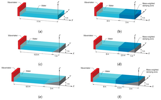
Figure 1.
Schematics. (a) NWT without a beach slope and a mass-weighted damping zone, (b) NWT with a mass-weighted damping zone without a beach slope, (c) NWT with a beach slope of 1:1, (d) NWT with a beach slope of 1:1 and a mass-weighted damping zone, (e) NWT with a beach slope of 1:3, and (f) NWT with a beach slope of 1:3 and a mass-weighted damping zone.
3.2. Numerical Results
3.2.1. Performance of the Mass-Weighted Damping Zone
In this section, the performance of the mass-weighted damping zone is verified using the NWT without beach slope model. To evaluate the accuracy of generated waves, two models are developed as shown in Figure 2a,b. The NWT of Case I-1 is modeled without a damping zone, and a mass-weighted damping zone is used in Case I-2.
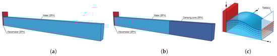
Figure 2.
(a) Case I-1: numerical wave tank without a mass-weighted damping zone. (b) Case I-2: numerical wave tank with a mass-weighted damping zone. (c) Spatial coordinate system in SPH simulation.
The fluid particles in both SPH simulation and experiment move along elliptical paths. Therefore, it is necessary to identify trajectories and sort the corresponding paths of particles that passed through the given coordinate x. The wave heights are measured from the highest and lowest bounds of the surface particle coordinates in the z-direction, and the horizontal and vertical velocities are calculated from the movements of the particles experiencing the highest or lowest displacements. The horizontal and vertical particle velocities of the numerical wave and resultant wave heights are measured at a specified coordinate as shown in Figure 2c.
The movements of the piston-type wavemaker are determined by Equations (21) and (22), and the wave parameters used in the simulation are listed in Table 3. The numerical waves are generated for 20 s in the simulation. To verify the NWT model with mass-weighted damping zone, the time history of the numerical wave height and particle velocities are compared with the analytical results.
Table 3.
Wave parameters in the numerical simulation Cases I-1 and I-2.
The numerical and analytical wave heights at x = 1.0 m, 2.0 m, and 4.0 m are shown in Figure 3a–c, respectively. As shown in Figure 3, the wave period and wave height of Case I-1 tend to decrease as the measurement positions are closer to the wavemaker. Compared with the analytical solution, the wave height at x = 1.0 m is smaller than 0.1 m, and that of x = 2.0 m is similarly calculated. The wave height increases up to 0.17 m, by 70%, after 9 s when the distance from the wavemaker x is 4.0 m. On the contrary, the numerical waves with the use of the mass-weighted damping zone are relatively steady and uniform with the amplitude of 0.05 m. At the measurement positions, however, the numerical wave profiles show slight constructive interference due to the reflected waves. The results in Figure 3c might repeat showing small fluctuation in the long-term analysis of wave profiles such as crests or troughs.
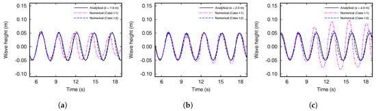
Figure 3.
Comparison of the numerical and analytical wave heights (a) at x = 1.0 m, (b) x = 2.0 m, and (c) x = 4.0 m.
The harmonic components of the numerical and analytical wave height at x = 4.0 m are illustrated in Figure 4. The first order component is dominant, and the others are negligibly small. The frequency of Cases I-1 and I-2 is 0.373 Hz which is calculated as 0.8% error compared with the analytical result. Due to the reflected waves, the wave frequency is not significantly disturbed in both cases, and however, the amplitude spectrum of Case I-1 is calculated as an error of 25%. The amplitude spectrum of Case I-2 with a mass-weighted damping zone is calculated as an error of 2.8%.
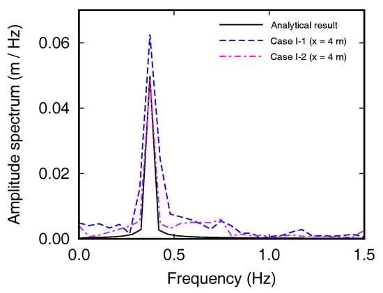
Figure 4.
Comparison of the numerical wave at x = 4.0 m in the frequency domain.
The horizontal and vertical velocities at x = 1.0 m, 2.0 m, and 4.0 m calculated with the use of the NWT, and solutions from linear wave theory are shown in Figure 5. Compared with the analytical solution, the horizontal velocities of Case I-1 are overestimated at every measurement position. For the vertical velocities, the tendency is analogous to wave heights, and the profile is jagged at x = 2.0 m and 4.0 m. However, results of the numerical wave tank using the mass-weighted damping zone, both horizontal and vertical velocities agree well with the analytical solutions.
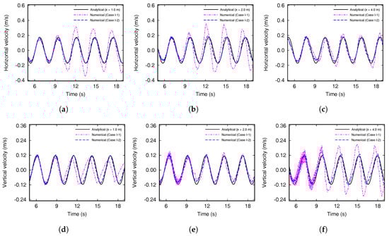
Figure 5.
Comparison of the numerical and analytical results of horizontal velocities (a) at x = 1.0 m, (b) x = 2.0 m, and (c) x = 4.0 m. Results of vertical velocities (d) at x = 1.0 m, (e) x = 2.0 m, and (f) x = 4.0 m.
Without the mass-weighted damping zone, the numerical wave profiles show constructive- or destructive interference due to the effect of the reflected wave and it cannot be uniformly calculated. However, using the mass-weighted damping zone, wave heights and velocities are similar to the theoretical formula, and wave profiles can be calculated regardless of the measurement positions. When using a mass-weighted damping zone, the selection of the damping coefficient is most important, and all the NWT model in the present section, is set to 1.5.
3.2.2. Effect of Initial Particle Spacing and Time Step
When the fluid is modeled using the smoothed particles, each particle replaces a volume. The accuracy of the results can be improved as the number of particles in the calculation range increases. However, increasing the number of smoothed particles causes a drastic increase in the calculation time. Therefore, initial particle spacing (IPS) and time step should be carefully selected for efficient analysis. To verify the effect of the IPS and time step on the accuracy of the numerical result, numerical analyses are performed using parameters in Table 3 and Table 4, and the numerical results are compared with the theoretical formulas.
Table 4.
Initial particle spacing and time step for parametric studies.
As listed in Table 4, the initial particle spacings of the NWT models with beach slope are set to be 2 cm, 4 cm, and 6 cm for Cases I-2, II-1, and II-2 respectively, and the time steps are set to be proportional to the initial particle spacing. The time histories of the wave height measured at 1 m from the wavemaker are shown in Figure 6a. In Cases I-2, II-1, and II-2, periods of the numerical wave show similar results with the analytical solutions and reflected waves are suppressed regardless of the initial particle spacings. However, the wave heights of Cases II-1 and II-2 show a difference at the wave through. If the particle spacing is 4 cm or more, the numerical results are calculated to be less accurate. The accuracy of numerical results increases as the initial particle spacing decreases, and the numerical model with IPS of 2 cm show good agreement. As shown in Figure 6a, the numerical results show that the accuracy significantly increases as the initial particle spacing decreases. Although the smoothed particles spaced smaller than 2 cm can provide more accurate results, the computation time exponentially increases with decreasing the initial particle spacing. As a result, there is the optimal particle spacing required to produce an accurate wave using the developed numerical wave tank. Therefore, the numerical model discretized with 2 cm of IPS is recommended for efficient analysis.
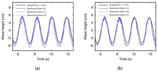
Figure 6.
Comparison of the numerical wave height with different the (a) initial particle spacings and (b) time steps.
The numerical wave height in Case II-1, II-3, and II-4 are shown in Figure 6b. As shown in Table 4, the initial particle spacing is fixed as 4 cm, and the time steps are changed to be 1.4 ms for Case II-3, and 1.7 ms for Case II-4, respectively. As aforementioned in Equation (14), the time step is calculated by dividing the minimum distance between the SPH elements by the wave-velocity of water, and this procedure is repeated at every calculation step. In general, the smaller the time step, the more accurate and stable calculation can be obtained, and the error decreases. Although the accuracy of the analysis results does not change clearly in Figure 6b, but the computational accuracy slightly increases in the wave trough. Therefore, by reducing the time step, the computational accuracy of the model with an initial particle spacing of 2 cm can be improved more. However, a value 10% smaller than the calculated time step is applied to the explicit analysis in LS-DYNA (Equation (15)). When the initial particle spacing is properly determined, a stable and efficient simulation can be performed with the automatically calculated time step.
3.2.3. Selection of Damping Coefficient
In the previous section, numerical simulations are performed using the mass-weighted damping zone installed in a vertical wall type of NWT as shown in Figure 2b. However, depending on the experimental conditions, beach slopes might be required at the right end of the wave tank. In the research of Machado et al. [], the effect of the reflected wave changes according to the beach slope at the right end of the NWT. Therefore, in order to accurately calculate the wave profile at all measurement positions regardless of the beach slope of the NWT, it is necessary to find proper damping coefficients () for each numerical model with different slope angles.
In this section, three different numerical wave tanks are modeled as shown in Figure 2b and Figure 7a,b, and optimal damping coefficients are suggested for each numerical model. The x-directional length of the water is modeled to be the same as the NWT without beach slope in Section 3.2.1, and the lateral area of the damping zones are modeled to be 3 m2 regardless of the beach slope. The beach slopes of the numerical models are shown in the Table 5.
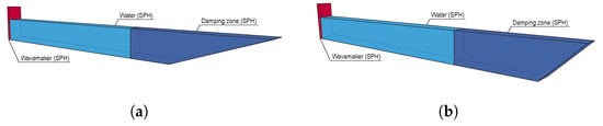
Figure 7.
(a) Case III-1: numerical wave tank using a mass-weighted damping zone with beach slope of 1:1. (b) Case III-2: numerical wave tank using a mass-weighted damping zone with beach slope of 1:3.
Table 5.
Numerical wave tank models with different beach slopes.
To estimate the optimal value of the damping coefficient for the NWT, the parametric studies are carried out varying the damping coefficient with 0.2 intervals from 0.3 to 2.3. Wave parameters in Table 3 are used, and the numerical wave heights are compared with the analytical results. The errors of wave height between the analytical data and numerical simulations are shown in Figure 8.
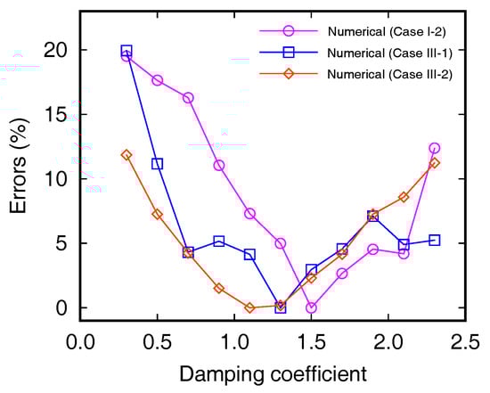
Figure 8.
Errors of numerical results for each model compared with analytical solution according to the damping coefficients ().
As shown in Figure 8, errors of the numerical wave height by varying the value of show a U-shaped curve in every case. For any shape of mass-weighted damping zone, there is a specific value that minimizes the wave height error caused by the reflected wave. When a value of the damping coefficient slightly larger or smaller than the optimal value is applied, the errors of the numerical wave height tend to increase compared with the theoretical equation. Therefore, the value of must be properly chosen to ensure that reflected wave can be damped at the damping zone. In the simulation of Case I-2, the error due to the reflected wave is minimized when is 1.5. For Cases III-1 and III-2, the smallest errors are calculated when is 1.3 and 1.1, respectively. As the beach slope of the mass-weighted damping zone becomes gentler, the smaller is needed. Because the beach slope exerts as a damper compared with the vertical wall-boundary. If a proper damping coefficient is applied, a semi-infinite wave without reflected wave can be generated irrespective of the shape of the mass-weighted damping zone.
3.3. Application
Ursell et al. [] generated the linear wave in the two regions of wave steepness: and , and compared the experimental results with the linear wave theory to evaluate the accuracy of the generated waves in the experimental wave flume. The wave height in the former range was measured within an error of 3–4%, and the wave height in the latter region was measured within an error of 10%. The numerical wave generated in Section 3.2.1 is included in the former range of Ursell et al. [] and covered in several previous studies. To evaluate the wave generating performance of the NWT, it is necessary to generate waves with various relative depths and wave steepness.
The water depth h is fixed at 1.0 m, and the wavenumber k is controlled, corresponding relative depths are ranged from 1 to 3. Also, to investigate the effect of the wave steepness, the target wave height of Cases IV are fixed as 0.1 m and that of Cases V are controlled to 0.2 m. The details of the wave parameters used in the simulation are listed in Table 6.
Table 6.
Wave parameters in the numerical simulations.
To confirm the dispersion relation of the generated waves, the wave height and the wavelength are calculated at x = 1 m and 5.36 m from the wavemaker, respectively, and the numerical results are compared with the dispersion formulation as shown in Figure 9. The numerical results are analogous to the dispersion relation, and however, the wavelengths are slightly overestimated than the target value in the case of the short-period wave such as Cases V-7 and V-8.
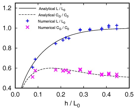
Figure 9.
Variation of wave dispersion parameters and for .
Figure 10a shows the wave height to stroke ratio () according to the relative depth at 1.0 m from the wavemaker, and Figure 10b indicates the errors between the numerical and theoretical results of the in Equation (21). As shown in Figure 10a, when a long-period wave with a relative depth smaller than 2 is generated, the agreement between the theoretical and the numerical results is good regardless of the target wave height. On the other hand, the differences between the theoretical equation and the numerical results in Cases V become higher when short-period waves with a relative depth of 2.5 or more is generated. In particular, Figure 10b shows that is calculated within an error of 1% for Cases IV-6 to IV-8, and the errors exceed 8% for Cases V-6 to V-8 when the relative depth is larger than 2.5. The relative depths of Cases IV-6 to IV-8 and Cases V-6 to V-8 are the same, but the errors show significant differences. Therefore, it is difficult to evaluate the wave generating performance of NWT by relative depth alone, and the additional criteria are required to determine the error when generating various wave heights.
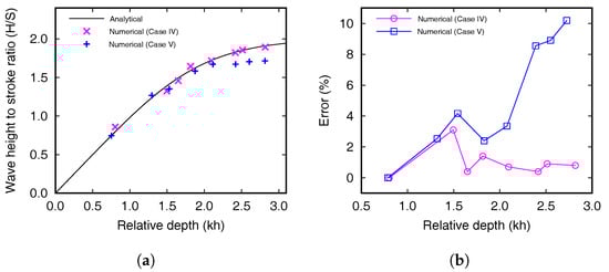
Figure 10.
Curves showing a comparison of (a) the wave height to stroke ratio and (b) errors obtained using the plane wavemaker theory and via numerical simulation.
For the target wave height of 0.1 m in Table 6, all the waves are included in the first range of steepness in Ursell et al. [], and the wave height to the stroke ratios obtained numerically are in close agreement with obtained theoretically; all the waves are generated within an error of 4% regardless of the relative depth as shown in Figure 10b. Cases V-1 and V-2 are included in the corresponding region, and the numerical wave height can be calculated within an error of 3.5%. On the other hand, the errors of Cases V-4 to V-8 change in proportion with the relative depth, i.e., when the wave steepness is included in the small wave steepness range of Ursell et al. [], the wave can be generated within an error of 4%, regardless of . When the target wave steepness is less than 0.07, the NWT with the use of the mass-weighted damping zone can calculate the wave height with an error of less than 5%, irrespective of the relative depth. As a result, NWT with mass-weighted damping zone model can calculate regular wave with wave steepness smaller than 0.1 within 10% error.
4. Experimental Verification
To verify the wave generating performance of the NWT using mass-weighted damping zone, we performed 17 cases of experiment using wave flume for various steepness and relative depth. This section includes the equipment used in the experiment and a comparison of the numerical results with the measured data.
4.1. Experiment Conditions
Experiments were conducted in the wave flume of the Physical Experiment Building at the Korea Institute of Ocean Science and Technology (KIOST), Busan. The waves were generated in an experimental wave flume with a length of 50 m, a width of 1.2 m, and a depth of 1.6 m with passive wave absorbers at both ends as shown in Figure 11a,b. The experimental wave flume is divided into three sections. The height of the wave flume is 1.65 m in the length of 10 m, and the bed of the wave flume is 1.25 m in the length of 20 m 50 m. In the section of 10 m 20 m, a slope was installed on the bed, and the depth of the water tank is gradually decreased from 1.65 m to 1.25 m. A piston-type wavemaker with the advantage of producing shallow and intermediate water waves was used in the experiment. The wavemaker was made by stainless steel and glass fiber reinforced plastic (GFRP) and weighed 85 kg with a height of 1.6 m and a width of 1.2 m. When the water depth is 1.0 m, the maximum stroke of the wavemaker and wave height are 1.2 m and 55 cm, respectively, and regular waves with the period range of 1.7 s to 3.0 s can be generated. More precise information of wavemaker and wave flume can be found in Oh and Lee [].
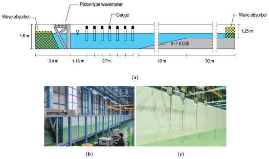
Figure 11.
(a) Schematic of the experimental wave flume, (b) experimental wave flume at KIOST [], and (c) capacitance type wave gauges.
A capacitance type wave gauge was installed 1.16 m upstream of the wavemaker plate, and six additional gauges were placed at 0.7 m intervals from the previous wave gauges as shown in Figure 11c. The external dimensions of the wave gauge were 60 mm in width, 128 mm in height, and 230 mm in length, and the maximum measuring wave height was 50 cm. The wave gauges were used to measure the wave properties such as the wave height and wave period, and the wavelengths were measured using gauges 2 and 7 with a distance of 3.5 m. The detailed location of the wave gauge is listed in Table 7, and the camera used in the experiment could be taken 6.5 frames per second.
Table 7.
Location of wave gauges from the wavemaker.
4.2. Comparison between Experimental, Numerical, and Analytical Results
In Section 3.3, the numerical wave heights with wave steepness greater than 0.07 are calculated an error of larger than 8% compared to the theoretical curve of the wave height-to-stroke ratio. In this section, to verify the NWT, waves were experimentally generated using the wave parameters in Table 6, and the wave height to stroke ratio is compared with the numerical results in Section 3.3 and Equation (21). The experimental results were obtained with the response of 20 s, and four snapshots of the regular wave were taken from Case IV-2.
Figure 12a,c,e,g show the propagation of the linear wave, and Figure 12b,d,f,h show the numerical results obtained at the identical times with the experiments. The propagation of the numerical wave demonstrates a good fidelity with the experiment snapshots. To verify the numerical results, the experimental measurements at three different coordinates (x = 1.16 m, 1.86 m, and 3.96 m) were compared. As shown in Figure 13a–c, the wave heights of all measured points were steady and uniform, and both numerical and experimental wave profiles show a good agreement with the experimental results.
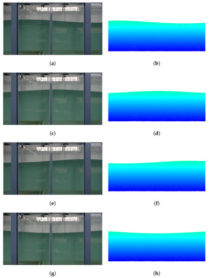
Figure 12.
Comparison of the linear waves in experiments (left) and numerical simulations (right) of Case IV-2.
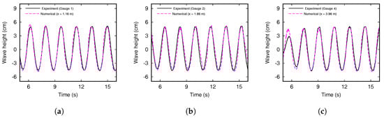
Figure 13.
Comparison of the numerical and experimental wave heights (a) at x = 1.16 m, (b) x = 1.86 m, and (c) x = 3.96 m (Case IV-2).
As described in Section 3.3, experiments were performed using the wave parameters in Table 6, and numerical and experimental results were compared. Figure 14a,b show the analytical, numerical, and experimental in accordance with the relative depth. For Cases IV-1 to IV-8, numerical and experimental results showed a good agreement with the theoretical formulas regardless of the target wave steepness. The experimental wave heights were calculated within an error of 4.1% that is in agreement with the errors presented by Ursell et al. []. For Cases V-1 to V-8, wave steepness was varied from 0.025 to 0.094, and the wave height-to-stroke ratio () is smaller than the analytical value when the wave steepness is larger than 0.067. The relative depths of Cases IV and V were changed in the range of 0.752 to 2.815. Both numerical and experimental wave height-to-stroke ratios of Cases IV-1 to IV-8 were accurately obtained regardless of the relative depth, but the results of Cases V-6 to V-8 were slightly underestimated if the relative depth is larger than 2.419. Water displaced by the wavemaker using the linear wave theory cannot produce sinusoidal waves with large wave height and short wavelength. Because the target wave steepness is large, the wave condition is inconsistent with the assumptions in the small-amplitude wave theory. To generate the linear wave, the target wave height should be considerably smaller than the wavelength and water depth. For Cases V-6 through V-8 with target wave steepness larger than 0.067, the wave height becomes similar to the target wavelength. The surface of the water pushed by the wavemaker is not sinusoidal, the crest and trough deform to be sharpened and widened, respectively, and nonlinear waves have smaller wave height than the predicted value. Therefore, the wave height-to-stroke ratio of the generated wave is slightly underestimated than the analytical solution as shown in Figure 14. Using the developed numerical wave tank, the applicable range of the linear wavemaker signal could be figured out. It should be noted that the linear wave theory is valid in the range of small wave steepness [], and linear waves can be accurately generated using the developed NWT if the target wave steepness is equal or smaller than 0.067.
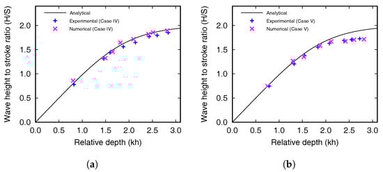
Figure 14.
Curves showing a comparison of the wave height to stroke ratio obtained using the wavemaker theory, experiment, and via numerical simulations. (a) Cases IV-1 to IV-8 and (b) Cases V-1 to V-8.
When the target wave height was larger than 10% of the target wavelength, the wave began to collapse right behind the wavemaker in the experimental wave flume. The height of the generated wave was lower than the predicted value, and this phenomenon was analogous to that observed in the experiment of Krvavica et al. []. To verify the wave breaking in the NWT, the wave is simulated for the wave parameters listed in Table 8.
Table 8.
Wave parameters for experiment and numerical simulation.
Figure 15a shows the moment in which a breaking wave was formed. Sequentially, Figure 15c,e,g present the developments of the breaking waves. It was observed that the water made a plunging breaker as soon as the wavemaker pushed the water. To verify the numerical simulation results, the experimental measurements were used for comparison. Figure 15b,d,f,h show the numerical results obtained at the identical times with the experiments. The regular wave is transformed to the breaking wave in the numerical simulation, and the shapes demonstrated a good fidelity with the experiment.
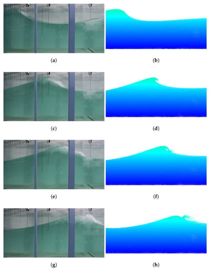
Figure 15.
Comparison of the breaking waves in experiments (left) and numerical simulations (right) of Case VI-1.
Figure 16a shows the wave height measured from the wave gauges installed at a distance of 1.16 m from the wavemaker, and the calculated wave height at the same position in the NWT model. Since the absorber installed at the left end of the experimental wave flume, it can be seen that there is no influence of the reflected wave on the measured data, and the wave reflection is effectively suppressed with the use of mass-weighted damping zone in the numerical wave tank. The measured wave height was 0.469 m, which was 8.04% smaller than the input wave height of 0.51 m. The wave height calculated using the NWT model was 0.455 m, which was calculated with an error of 2.99% compared to the experimental results. The second wave height gauge (x = 1.86 m) was located at 0.7 m away from the first wave height gauge (x = 1.16 m) and the measured wave heights are shown in Figure 16b. The wavelength was calculated from the data of the described wave gauges, and the measurement value was 3.69 m. In the NWT model, the wavelength was calculated by using the numerical data at the same position where the wave height gauge was installed, and the calculated wavelength was 3.51 m which was calculated with an error of 4.6% compared to the experimental results. The errors in the numerical results with respect to the experimental results were summarized in Table 9.
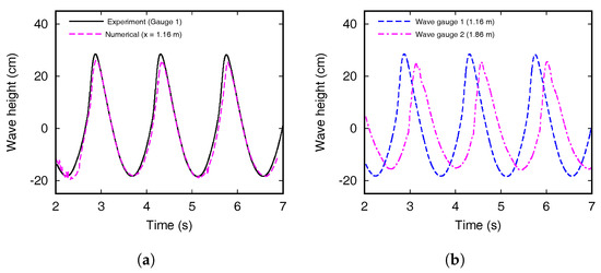
Figure 16.
(a) Comparison of the wave heights in experiments and numerical simulations (Case VI-1). (b) Measured wave heights from the wave gauges 1 and 2 (Case VI-1).
Table 9.
Errors in the wave parameters between experiment and numerical results of Case VI-1.
As shown in Figure 15 and listed in Table 9, when the target wave steepness is larger than 0.1, the wave height, wavelength, and the wave steepness of the experimental and numerical results are underestimated than that by the linear wave theory due to the breaking phenomenon []. As observed in the experiment, the linear wave theory is valid in the range of small wave steepness []. These results indicate that the developed NWT using the mass-weighted damping zone can simulate the identical waves with those in the experiment when the damping is properly imposed.
5. Summary and Conclusions
The aim of this study is to generate waves with short periods, large relative depth, and large wave steepness, which are rarely discussed so far, and to effectively suppress the reflected wave using mass-weighted damping zone. Waves with the various relative depths and wave steepnesses are numerically and experimentally generated, and results are compared with the analytical solutions to optimize the numerical variables including a damping coefficient, initial particle spacing, beach slopes, and calculation time steps. Although numerical wave tank (NWT) discretized by smoothed particles with mass-weighted damping is modeled to have a shorter length than that of the experimental wave flume, but generate uniform and accurate regular waves when compared with experimental results.
Parametric studies are performed by varying the initial spacing of the smoothed particles, computation time steps, beach slope, and damping coefficient (). The numerical wave profiles are more accurately calculated when the initial spacing of the SPH elements constituting the water is discretized more densely, but a significant analysis time is required with very densely populated particles. In fact, with finer particle arrangements, the computation cost increases drastically. Accurate waves can be calculated by setting the particle spacing as 2 cm and the time step as 90% of the critical time step. As the slope of the damping zone becomes less steep, the reflection effect decreases because the beach functions as a damper. Therefore, the NWT with the weak slope requires a smaller damping coefficient. By calculating the least-squares error, we found that there is an optimal damping coefficient regarding the beach slope of the NWT. With the initial particle spacing as 0.02 m, 90% of the critical time step for the time integration, and of 1.5 for damping, the calculation yields efficiently accurate results without wave reflection.
To verify the wave generating performance, target wave height and periods are changed in both simulation and experiment. When the target wave steepness is equal or smaller than 0.067, both numerical and experimental waves are accurately generated irrespective of the relative depth. However, when the target wave steepness is larger than 0.067, both experimental and numerical wave height-to-stroke ratios are slightly underestimated than the analytical value, and the waves start to break.
The present study indicates that the developed numerical wave tank with the mass-weighted damping zone is very useful to accurately generate waves of different wave steepnesses from linear to breaking waves, and the numerical results are consistent with experimental results. Further development of the NWT model will be beneficial to solve practical offshore problems with various periods, heights, and wave steepnesses. Also, large-scale problems can be efficiently calculated using the NWT model that has shorter length than that of the experimental setup.
Author Contributions
Conceptualization, S.L. and J.-W.H.; investigation, S.L.; methodology, S.L.; software, S.L.; validation, S.L.; visualization, S.L.; writing—original draft preparation, S.L. and J.-W.H.; writing—review and editing, S.L. and J.-W.H. All authors have read and agreed to the published version of the manuscript.
Funding
This work was supported by the National Research Foundation of Korea (NRF) Grant funded by the Korean Government (Ministry of Science and ICT) (No. 2017R1A5A1014883).
Conflicts of Interest
The authors declare no conflict of interest.
References
- De Antonio, F.O. Wave energy utilization: A review of the technologies. Renew. Sustain. Energy Rev. 2010, 14, 899–918. [Google Scholar]
- Tian, X.; Wang, Q.; Liu, G.; Deng, W.; Gao, Z. Numerical and Experimental Studies on a Three-Dimensional Numerical Wave Tank. IEEE Access 2018, 6, 6585–6593. [Google Scholar] [CrossRef]
- Manenti, S.; Petrini, F. Dynamic analysis of an offshore wind turbine: Wind-waves nonlinear interaction. In 12th Biennial International Conference on Engineering, Construction, and Operations in Challenging Environments; and Fourth NASA/ARO/ASCE Workshop on Granular Materials in Lunar and Martian Exploration; ASCE: Honoluu, HI, USA, 2010; pp. 2014–2026. [Google Scholar]
- Petrini, F.; Manenti, S.; Gkoumas, K.; Bontempi, F. Structural Design and Analysis of Offshore Wind Turbines from a System Point of View. Wind. Eng. 2010, 34, 85–107. [Google Scholar] [CrossRef]
- Lee, S.; Hong, J.W. Parametric studies on smoothed particle hydrodynamic simulations for accurate estimation of open surface flow force. Int. J. Nav. Archit. Ocean. Eng. 2020, 12, 85–101. [Google Scholar] [CrossRef]
- Galvin, C.J., Jr. Wave-Height Prediction for Wave Generators in Shallow Water; Technical Report; U.S. Army Coastal Engineering Research Center: Washington, DC, USA, 1964. [Google Scholar]
- Havelock, T. LIX. Forced surface-waves on water. Lond. Edinb. Dublin Philos. Mag. J. Sci. 1929, 8, 569–576. [Google Scholar] [CrossRef]
- Dean, R.G.; Dalrymple, R.A. Water Wave Mechanics for Engineers and Scientists; World Scientific Publishing Company: Singapore, 1991; Volume 2. [Google Scholar]
- Goda, Y. Travelling secondary wave crests in wave channels. Port Harb. Res. Inst. Minist. Transp. Jpn. 1967, 13, 32–38. [Google Scholar]
- Madsen, O.S. On the generation of long waves. J. Geophys. Res. 1971, 76, 8672–8683. [Google Scholar] [CrossRef]
- Ursell, F.; Dean, R.G.; Yu, Y.S. Forced small-amplitude water waves: A comparison of theory and experiment. J. Fluid Mech. 1960, 7, 33–52. [Google Scholar] [CrossRef]
- Schäffer, H.A. Second-order wavemaker theory for irregular waves. Ocean. Eng. 1996, 23, 47–88. [Google Scholar] [CrossRef]
- Monaghan, J.J. Simulating Free Surface Flows with SPH. J. Comput. Phys. 1994, 110, 399–406. [Google Scholar] [CrossRef]
- Dalrymple, R.A.; Knio, O. SPH Modelling of Water Waves. In Proceedings of 4th Conference on Coastal Dynamics; ASCE: Honoluu, HI, USA, 2001; Volume 1, pp. 779–787. [Google Scholar]
- Dalrymple, R.; Rogers, B. Numerical modeling of water waves with the SPH method. Coast. Eng. 2006, 53, 141–147. [Google Scholar] [CrossRef]
- Khayyer, A.; Gotoh, H.; Falahaty, H.; Shimizu, Y. Towards development of enhanced fully-Lagrangian mesh-free computational methods for fluid-structure interaction. J. Hydrodyn. 2018, 30, 49–61. [Google Scholar] [CrossRef]
- Silvester, T.B.; Cleary, P.W. Wave-structure interaction using smoothed particle hydrodynamics. In Proceedings of the Fifth International Conference on CFD in the Process Industries, Mlbourne, Australia, 13–15 December 2006; pp. 13–15. [Google Scholar]
- Manenti, S.; Wang, D.; Domínguez, J.M.; Li, S.; Amicarelli, A.; Albano, R. SPH Modeling of Water-Related Natural Hazards. Water 2019, 11, 1875. [Google Scholar] [CrossRef]
- Manenti, S.; Amicarelli, A.; Todeschini, S. WCSPH with limiting viscosity for modeling landslide hazard at the slopes of artificial reservoir. Water 2018, 10, 515. [Google Scholar] [CrossRef]
- Verbrugghe, T.; Stratigaki, V.; Altomare, C.; Domínguez, J.; Troch, P.; Kortenhaus, A. Implementation of open boundaries within a two-way coupled SPH model to simulate nonlinear wave–structure interactions. Energies 2019, 12, 697. [Google Scholar] [CrossRef]
- Wang, H.W.; Huang, C.J.; Wu, J. Simulation of a 3D numerical viscous wave tank. J. Eng. Mech. 2007, 133, 761–772. [Google Scholar] [CrossRef]
- Gotoh, H.; Khayyer, A. On the state-of-the-art of particle methods for coastal and ocean engineering. Coast. Eng. J. 2018, 60, 79–103. [Google Scholar] [CrossRef]
- Didier, E.; Neves, M.G. A semi-infinite numerical wave flume using Smoothed Particle Hydrodynamics. Int. J. Offshore Polar Eng. 2012, 22, 193–199. [Google Scholar]
- Altomare, C.; Domínguez, J.M.; Crespo, A.; González-Cao, J.; Suzuki, T.; Gómez-Gesteira, M.; Troch, P. Long-crested wave generation and absorption for SPH-based DualSPHysics model. Coast. Eng. 2017, 127, 37–54. [Google Scholar] [CrossRef]
- Ren, B.; Wen, H.; Dong, P.; Wang, Y. Numerical simulation of wave interaction with porous structures using an improved smoothed particle hydrodynamic method. Coast. Eng. 2014, 88, 88–100. [Google Scholar] [CrossRef]
- He, M.; Gao, X.F.; Xu, W.H. Numerical simulation of wave-current interaction using the SPH method. J. Hydrodyn. 2018, 30, 535–538. [Google Scholar] [CrossRef]
- Wen, H.; Ren, B.; Dong, P.; Wang, Y. A SPH numerical wave basin for modeling wave-structure interactions. Appl. Ocean. Res. 2016, 59, 366–377. [Google Scholar] [CrossRef]
- Domínguez, J.M.; Crespo, A.J.; Hall, M.; Altomare, C.; Wu, M.; Stratigaki, V.; Troch, P.; Cappietti, L.; Gómez-Gesteira, M. SPH simulation of floating structures with moorings. Coast. Eng. 2019, 153, 103560. [Google Scholar] [CrossRef]
- Prasad, D.D.; Ahmed, M.R.; Lee, Y.H.; Sharma, R.N. Validation of a piston type wave-maker using Numerical Wave Tank. Ocean. Eng. 2017, 131, 57–67. [Google Scholar] [CrossRef]
- Finnegan, W.; Goggins, J. Numerical simulation of linear water waves and wave–structure interaction. Ocean. Eng. 2012, 43, 23–31. [Google Scholar] [CrossRef]
- Machado, F.M.M.; Lopes, A.M.G.; Ferreira, A.D. Numerical simulation of regular waves: Optimization of a numerical wave tank. Ocean. Eng. 2018, 170, 89–99. [Google Scholar] [CrossRef]
- Altomare, C.; Tagliafierro, B.; Dominguez, J.; Suzuki, T.; Viccione, G. Improved relaxation zone method in SPH-based model for coastal engineering applications. Appl. Ocean. Res. 2018, 81, 15–33. [Google Scholar] [CrossRef]
- Zhang, H.C.; Liu, S.X.; Li, J.X.; Wang, L. Establishment of Numerical Wave Flume Based on the Second-Order Wave-Maker Theory. China Ocean. Eng. 2019, 33, 160–171. [Google Scholar] [CrossRef]
- Dong, C.M.; Huang, C.J. Generation and propagation of water waves in a two-dimensional numerical viscous wave flume. J. Waterw. Port Coast. Ocean. Eng. 2004, 130, 143–153. [Google Scholar] [CrossRef]
- Wu, N.J.; Tsay, T.K.; Young, D. Meshless numerical simulation for fully nonlinear water waves. Int. J. Numer. Methods Fluids 2006, 50, 219–234. [Google Scholar] [CrossRef]
- Anbarsooz, M.; Passandideh-Fard, M.; Moghiman, M. Fully nonlinear viscous wave generation in numerical wave tanks. Ocean. Eng. 2013, 59, 73–85. [Google Scholar] [CrossRef]
- Lind, S.; Xu, R.; Stansby, P.; Rogers, B. Incompressible smoothed particle hydrodynamics for free-surface flows: A generalised diffusion-based algorithm for stability and validations for impulsive flows and propagating waves. J. Comput. Phys. 2012, 231, 1499–1523. [Google Scholar] [CrossRef]
- Lucy, L.B. A Numerical Approach to the Testing of the Fission Hypothesis. Astron. J. 1977, 82, 1013–1024. [Google Scholar] [CrossRef]
- Gingold, R.A.; Monaghan, J.J. Smoothed Particle Hyrodynamics: Theory and Application to Non Spherical Star. Mon. Not. R. Astron. Soc. 1977, 181, 375–389. [Google Scholar] [CrossRef]
- Cummins, S.J.; Silvester, T.B.; Cleary, P.W. Three-dimensional wave impact on a rigid structure using smoothed particle hydrodynamics. Int. J. Numer. Methods Fluids 2012, 68, 1471–1496. [Google Scholar] [CrossRef]
- Monaghan, J.J.; Lattanzio, J.C. A refined particle method for astrophysical problems. Astron. Astrophys. 1985, 149, 135–143. [Google Scholar]
- Liu, M.B.; Liu, G.R. Smoothed Particle Hydrodynamics (SPH): An Overview and Recent Developments. Arch. Comput. Methods Eng. 2010, 17, 25–76. [Google Scholar] [CrossRef]
- Liu, G.R.; Liu, M.B. Smoothed Particle Hydrodynamics: A Meshfree Particle Method; World Scientific: Singapore, 2003. [Google Scholar]
- Hallquist, J.O. LS-Dyna Keyword User’s Manual; Livermore Software Technology Corporation: Livermore, CA, USA, 2007. [Google Scholar]
- Joubert, J.C.; Wilke, D.N.; Govender, N.; Pizette, P.; Tuzun, U.; Abriak, N.E. 3D gradient corrected SPH for fully resolved particle–fluid interactions. Appl. Math. Model. 2020, 78, 816–840. [Google Scholar] [CrossRef]
- Shi, C.; An, Y.; Wu, Q.; Liu, Q.; Cao, Z. Numerical simulation of landslide-generated waves using a soil–water coupling smoothed particle hydrodynamics model. Adv. Water Resour. 2016, 92, 130–141. [Google Scholar] [CrossRef]
- Manenti, S.; Pierobon, E.; Gallati, M.; Sibilla, S.; D’Alpaos, L.; Macchi, E.; Todeschini, S. Vajont disaster: Smoothed particle hydrodynamics modeling of the postevent 2D experiments. J. Hydraul. Eng. 2016, 142, 05015007. [Google Scholar] [CrossRef]
- Altomare, C.; Crespo, A.J.; Domínguez, J.M.; Gómez-Gesteira, M.; Suzuki, T.; Verwaest, T. Applicability of smoothed particle hydrodynamics for estimation of sea wave impact on coastal structures. Coast. Eng. 2015, 96, 1–12. [Google Scholar] [CrossRef]
- Libersky, L.D.; Petschek, A.G.; Carney, T.C.; Hipp, J.R.; Allahdadi, F.A. High strain Lagrangian hydrodynamics: A three-dimensional SPH code for dynamic material response. J. Comput. Phys. 1993, 109, 67–75. [Google Scholar] [CrossRef]
- Liu, X.; Liu, S.; Ji, H. Numerical research on rock breaking performance of water jet based on SPH. Powder Technol. 2015, 286, 181–192. [Google Scholar] [CrossRef]
- Biesel, F.; Suquet, F. Etude theorique d’un type d’appareil a la houle. La Houille Blanche 1951, 2, 157–160. [Google Scholar]
- Frigaard, P.; Andersen, T.L. Wave Generation Software AwaSys 5; DCE Technical Reports; Aalborg University: Aalborg, Denmark, 2010; Volume 64. [Google Scholar]
- Hallquist, J.O. LS-DYNA Theory Manual; Livermore Software Technology Corporation: Livermore, CA, USA, 2006. [Google Scholar]
- Oh, S.H.; Lee, D.S. Two-Dimensional Wave Flume with Water Circulating System for Controlling Water Level. J. Korean Soc. Coast. Ocean. Eng. 2018, 30, 337–342. [Google Scholar] [CrossRef]
- Krvavica, N.; Ružić, I.; Ožanić, N. New approach to flap-type wavemaker equation with wave breaking limit. Coast. Eng. J. 2018, 60, 69–78. [Google Scholar] [CrossRef]
© 2020 by the authors. Licensee MDPI, Basel, Switzerland. This article is an open access article distributed under the terms and conditions of the Creative Commons Attribution (CC BY) license (http://creativecommons.org/licenses/by/4.0/).