Wind-Induced Currents in the Gulf of California from Extreme Events and Their Impact on Tidal Energy Devices

Abstract

Tidal renewable energy is a promising alternative energy resource, and marginal seas are known as excellent sites for tidal energy exploitation. In-stream and tidal energy devices are less exposed to extreme weather events than wind energy. Nevertheless, during tropical storms, the currents may intensify to levels that threaten the integrity of the devices. This paper presents Hurricane Odile and its impact on the currents in the Gulf of California (GC) as a worst case scenario. A methodology to analyze the impact and its potential effects on tidal energy converters installed within the region are presented. The analysis is based on predictions obtained with a 3D shallow water model forced by tides and the meteorological conditions generated by Odile. A tidal model with no wind forcing was used for validation of the tidal model predictions. After validation, the two models were used to analyze the maximum anomaly in surface currents and sea surface height caused by the passage of Odile, and to analyze at which depth the devices could be deemed safe from any impact of the hurricane. Some anomalies extended throughout the water column, even in the deep regions of the GC. This paper highlights the importance of including the meteorological forcing in evaluations of tidal range or in-stream renewable energy resources and introduces new measures of device exposure to the current anomalies.

1. Introduction

Tidal and ocean currents can have a significant contribution to the global renewable energy production. In the case of tidal currents in particular, their predictability and continuous availability make them a key component in the renewable energy mix, and while tidal current variability in a one to four hour time window is large, tidal currents have very low variability over monthly to yearly timescales [1]. Efforts are underway to exploit both tidal and ocean current energy resources, ranging from the development of devices operating at different current speed ranges and water depths [2], increasing performance [3], and reducing costs [4]. At the same time, resources have to be characterized and optimal sites identified [1,5]. A vital component in the identification of optimal sites, is the analysis of potential device damage by extreme events. In tropical regions, for example, tropical cyclones and hurricanes pose a significant threat to offshore infrastructure. Whilst the risk is severe for offshore wind turbines [6], the high winds and atmospheric pressure fluctuations may still influence the currents in the surface and sometimes to considerable depth [7].

The Gulf of California (GC) is the only marginal sea in the Pacific Northeast and is expected to be an excellent site for tidal energy exploitation. The GC has the largest tidal range in Mexico [8], and potentially offers plenty of excellent locations for the installation of in-stream devices [9]. One advantage of the GC is that the return period of tropical storms, and particularly of hurricanes, is lower than in any other marine regions of Mexico [10]. Despite this, some major tropical storms, such as Hurricane Odile in September 2014, have travelled towards and into the Gulf, causing severe damage [11]. Hurricane Odile, with a return period of around 25 years in the Baja California Peninsula, is also known as the third major storm and the most destructive hurricane to make landfall in this region during the satellite era [11].

In the present work, the impact of Hurricane Odile on the currents within the Gulf of California—measured in terms of the following indicators: current anomalies, depth of anomaly and temporal exposure (the period when the hurricane affects the area)—is evaluated using a numerical model, over the domain shown in Figure 1. The aim is to assess how changes in these indicators affect the selection of tidal energy converters (TECs). For example, if the current anomaly remains near the surface, then TECs that can dive into deeper water to evade this anomaly can mitigate the risk of damage by tropical storms. If, on the other hand, the temporal exposure is short, then towing away the TECs for a short time may be feasible. If, in contrast, the anomaly penetrates most of the water column and the temporal exposure is long, then only TECs that can withstand the expected forces, potentially well beyond the standard operating conditions, will have to be considered. A TEC plant shutdown will, undoubtedly, harm the local economy and on energy security.

The paper is organized as follows. In Section 2, the shallow-water model and model set-up, the tidal forcing conditions, and the wind data processing are described. In Section 4, we present validations of the tidal model, the visualization and evaluation of the change in currents due to the hurricane, and the spatiotemporal extent of the anomalies. The implications of these results on TEC survivability issues, particularly for TECs installed within the GC, are discussed.

2. Methodology

The shallow-water model Delft3d [12] was used in this study to analyze three different forcing scenarios—tidal forcing with no wind, tidal forcing with wind climatology, and tidal forcing with the wind and atmospheric pressure field conditions during hurricane Odile (10–19 September 2014). The wind and pressure fields were obtained from a numerical weather forecasting model prediction for the period. The current anomalies, derived from the currents predicted by these three model runs, and their temporal-spatial characteristics were then compared and contrasted. The monthly surface wind climatology for the whole year of 2014 is available as a supplement to this publication, because it may be useful for a whole range of different studies.

2.1. The Model

The model domain is the marine region between the Colorado River Delta, located around (32${}^{\circ }$ N 115${}^{\circ }$ W), and the southern boundary of the grid shown in Figure 1, which extends from around (24${}^{\circ }$30′ N 107${}^{\circ }$50′ W) to (23${}^{\circ }$04′ N 109${}^{\circ }$35′ W). This domain may be divided in the Upper Gulf of California, the Great Island (or Midriff) Region, and the Southern Gulf of California [13]. Taking into account these regions, the Gulf of California is 1100 km long and around 150–200 km wide. The Upper Gulf of California is the very shallow (depth < 30 m) region north of 31${}^{\circ }$ N. the Great Island Region consists of a group of islands separated by narrow channels and sills with maximum depths of 300–600 m. In the Southern Gulf of California, the continental shelf is very narrow, and water depth of the channels and basins can be up to 3000 m. Stratification in the Gulf of California plays a role in the overall dynamics of the Gulf. In the mouth of the Gulf, the mixed layer depth can vary from 10–40 m. In the northern Gulf the mixed layer can vary between 100 m in the Delfin basin and 50 m in the Wagner basin, for example Reference [13]. The energetically dominant signal, however, is barotropic, in particular in the upper Gulf.

Delft3d solves the incompressible Navier-Stokes equations under the shallow water and the Boussinesq approximations, which consist of the following three assumptions:

• the vertical accelerations are neglected in the momentum equations;
• the momentum conservation equation in the vertical is replaced by a balance equation for the pressure field, and;
• the vertical velocities are computed from the continuity equation.

Temperature changes and salinity were not included in this model configuration. The default version of Delft3d uses curvilinear coordinates in the horizontal dimensions and $\sigma$-coordinates in the vertical dimension [14]. The curvilinear coordinates may be in (spherical) WGS84, in (local) UTM, or some other local coordinates. The $\sigma$ coordinate is defined as:

$$\sigma =\frac{z-\zeta }{d+\zeta }=\frac{z-\zeta }{H},$$

(1)

where z, $\zeta$, d, and H denote the vertical coordinate in physical space, the free surface elevation above the reference plane (at $z=0$), the depth below the reference plane, and the total water depth, respectively. By convention, $\sigma =-1$ at the bottom and $\sigma =0$ at the free surface. In this model set-up, the grid (shown in Figure 1, as mentioned above), has 63 by 183 grid points in the horizontal and between 25 and 34 grid points in the vertical—this depends on the surface resolution, as will be explained in Section 4.1.

The conservation equations will be expressed here in terms of the spherical coordinates $(\lambda ,\varphi ,R)$, with $\lambda$ being the longitude, $\varphi$ the latitude, and $R=$ 6378.137 km (WGS84) the radius of the Earth [15]. Then, the depth-averaged continuity equation,

$$\frac{\partial \zeta }{\partial t}+\frac{1}{R^{2}cos\varphi }\frac{\partial \left[\left(d+\zeta \right)UR\right]}{\partial \lambda }+\frac{1}{R^{2}cos\varphi }\frac{\partial \left[\left(d+\zeta \right)VRcos\varphi \right]}{\partial \varphi }=0,$$

(2)

is derived by integrating over the vertical coordinate the continuity equation for incompressible flows, with ${\displaystyle U={\int }_{-1}^{0}ud\sigma }$ and ${\displaystyle V={\int }_{-1}^{0}vd\sigma }$ being the depth-averaged velocities. The horizontal momentum equations are

$$\begin{array}{c}\hfill \frac{\partial u}{\partial t}+\frac{u}{Rcos\varphi }\frac{\partial u}{\partial \lambda }+\frac{v}{R}\frac{\partial u}{\partial \varphi }+\frac{\omega }{d+\zeta }\frac{\partial u}{\partial \sigma }-\frac{v^2}{R^{2}cos\varphi }\frac{\partial R}{\partial \lambda }+\frac{uv}{R^{2}cos\varphi }\frac{\partial (Rcos\varphi )}{\partial \varphi }-fv=\\ \hfill -\frac{1}{\rho Rcos\varphi }{P}_{\lambda }+F_{\lambda }+\frac{1}{{\left(d+\zeta \right)}^2}\frac{\partial }{\partial \sigma }\left({\nu }_v\frac{\partial u}{\partial \sigma }\right)+M_{\lambda }\hspace{1em}\end{array}$$

(3)

and

$$\begin{array}{c}\hfill \frac{\partial v}{\partial t}+\frac{u}{Rcos\varphi }\frac{\partial v}{\partial \lambda }+\frac{v}{R}\frac{\partial v}{\partial \varphi }+\frac{\omega }{d+\zeta }\frac{\partial v}{\partial \sigma }-\frac{uv}{R^{2}cos\varphi }\frac{\partial R}{\partial \lambda }+\frac{u^2}{R^{2}cos\varphi }\frac{\partial (Rcos\varphi )}{\partial \varphi }+fu=\\ \hfill -\frac{1}{\rho R}{P}_{\varphi }+F_{\varphi }+\frac{1}{{\left(d+\zeta \right)}^2}\frac{\partial }{\partial \sigma }\left({\nu }_v\frac{\partial v}{\partial \sigma }\right)+M_{\varphi }\hspace{1em},\end{array}$$

(4)

where ${\nu }_v$, $P_{\lambda ,\varphi }$, $F_{\lambda ,\varphi }$, and $M_{\lambda ,\varphi }$, denote vertical eddy viscosity, pressure gradients, forces from unbalanced Reynolds stresses and external forcing (wind), respectively. In a $\sigma$ coordinate system such as the one used here, the vertical velocity, $\omega$, is computed from the continuity equation

$$\frac{\partial \zeta }{\partial t}+\frac{1}{R^{2}cos\varphi }\frac{\partial \left[\left(d+\zeta \right)uR\right]}{\partial \lambda }+\frac{1}{R^{2}cos\varphi }\frac{\partial \left[\left(d+\zeta \right)vRcos\varphi \right]}{\partial \varphi }+\frac{\partial \omega }{\partial \sigma }=0.$$

(5)

A k-$ϵ$ turbulence closure model was used with constant horizontal eddy viscosity of 2 ${\mathrm{m}}^2/\mathrm{s}$, and a constant Chézy bottom friction coefficient of 45 $\sqrt{m}/s$ was applied. The simulation timestep was 0.5 min.

2.2. The Wind Forcing

At the surface of the sea, the boundary conditions for the momentum equations are

$$\begin{array}{ccc}\hfill \frac{{\nu }_v}{H}{\left.\frac{\partial u}{\partial \sigma }\right|}_{\sigma =0}& =& \frac{{\rho }_a}{\rho }{C}_d{U}_{10}^{2}cos\theta \hfill \end{array}$$

(6)

$$\begin{array}{ccc}\hfill \frac{{\nu }_v}{H}{\left.\frac{\partial v}{\partial \sigma }\right|}_{\sigma =0}& =& \frac{{\rho }_a}{\rho }{C}_d{U}_{10}^{2}sin\theta ,\hfill \end{array}$$

(7)

where ${\rho }_a$, $U_{10}$, and $C_d=0.0025$ denote the density of air, the 10-meter wind speed and the wind drag coefficient, respectively. The drag coefficient is still a matter of active research (cf. References [16,17]). The current drag coefficient value is well in the range of the values reported by References [16,17,18]. The model does not contain wave interactions, and hence any wave contribution has to be included through the wind forcing. The drag coefficient may appear high, however, in coastal settings the drag coefficient can increase relative to its value in the open ocean [18]. For higher resolution modelling it should indeed be revised, to take the different drag coefficients observed in the different sectors around the hurricane into account.

The wind and surface pressure data was taken from the North American Mesoscale model (NAM) with 12 km resolution. Hourly forecasts from the four daily forecast runs at UTC 00:00, 6:00, 12:00, and 18:00 were used, except for the 13 September and UTC 07:00–11:00 19 August, where the NAM data is not available. This gap was filled with data from the North American Regional Reanalysis (NARR) at three hourly temporal resolution. Representative wind fields for four dates are shown in Figure 2. Also shown is the trajectory of hurricane Odile and its current location. The reversal of the wind direction, when compared to the climatology—presented next—can be observed. The wind speeds are also significantly higher, as expected.

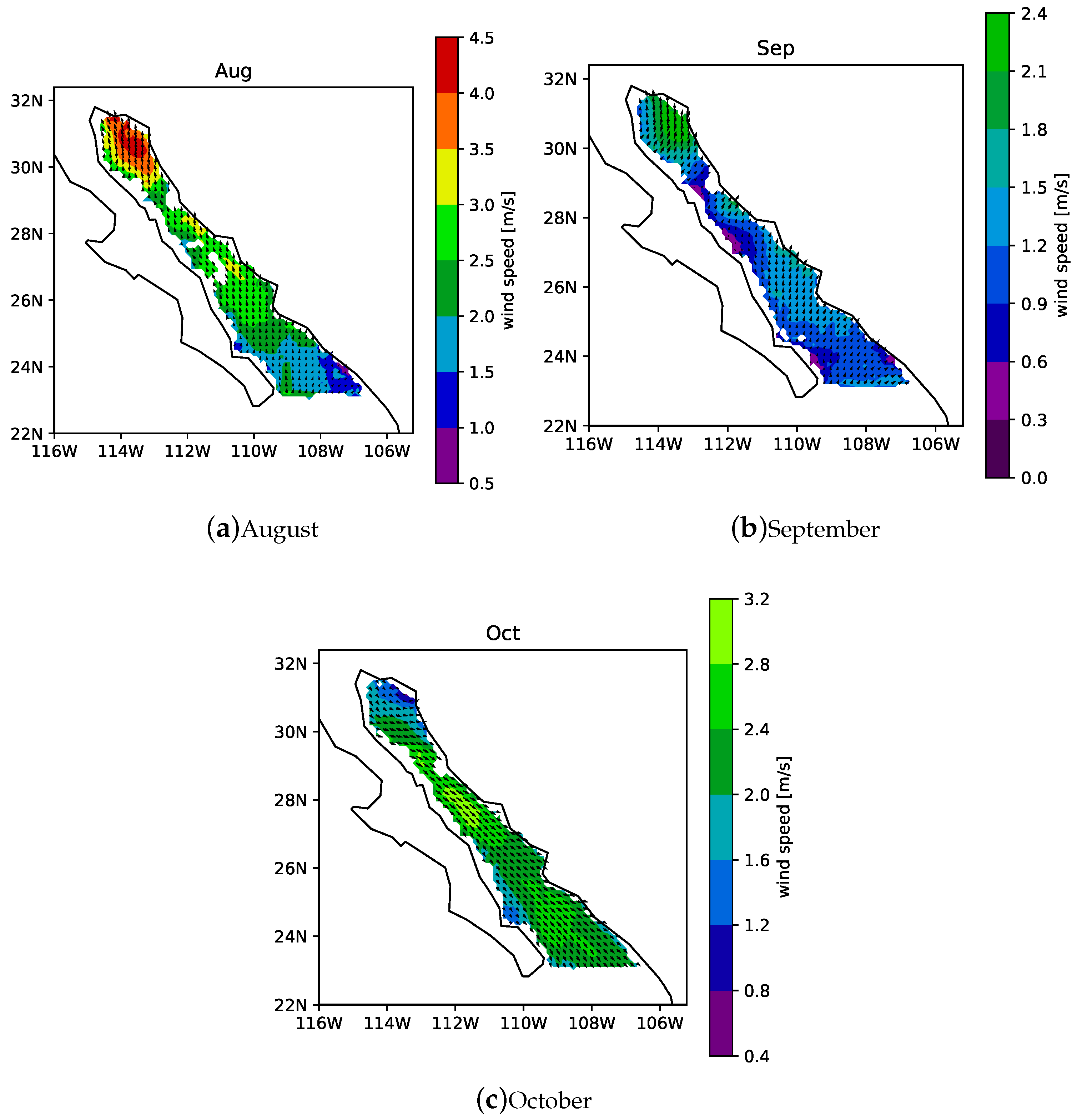
2.3. Surface Wind Climatology

The climatology of the Gulf is strongly seasonal. Focusing on the Monsoon period (July to September), Reference [19] generated a climatology for the Gulf of California using five years of QuickSCAT winds. Their climatology resolves the influence of the peninsula of Baja California and the dominant wind field patterns, together with the strong seasonal signal in the winds over the Gulf of California, which have also been identified in previous studies [20,21]. In the meantime, the availability of data sources has improved, and data from high–resolution weather models, reanalysis, and remote sensing is now available.

A climatology was generated for each month, as the standard September/October/November climatology would not be representative of the winds in September. The climatology for August, September, and October are reproduced in Figure 3.

The wind climatology data sources and their temporal coverage are shown in Figure 4. The data sources comprise five model datasets, UPSCALE, CSFR, CSF2, NARR and NAM, and four satellite products: CCMP, WIND-GLO, CERSATV4 and CERSATV5. These data sources are introduced in the following.

2.3.1. UK on PRACE—Weather-Resolving Simulations of Climate for globAL Environmental Risk (UPSCALE) Dataset

The UPSCALE [22,23] dataset is a global dataset with N512 resolution (1024 × 768 grid points East-West × North-South, ${0.23438}^{\circ }$ in latitude and ${0.3516}^{\circ }$ degrees in longitude). The Hadley Centre Global Environment Model version 3 (HadGEM3)—Global Atmosphere (GA) 3.0, Global Land (GL) 3.0 configuration of the Met Office Unified Model (MetUM) version 8.0 was used to generate the data, as documented in Walters et al. [24]. The configuration is set to reproduce the actual climate from Feb. 1985 to Dec. 2011. Instantaneous winds were obtained every three hours, are then averaged over the respective months.

2.3.2. North American Mesoscale Forecast System (NAM)

The NAM is a numerical weather prediction (NWP) model run by the US National Weather Service– National Centers for Environmental Prediction (NCEP), covering North America. It is using the MESO ETA Model [25]. The spatial resolution is 12km on the Advanced Weather Interactive Processing System (AWIPS) Lambert conformal grid over the Contiguous United States (CONUS). The data was re-gridded with bi-linear interpolation onto a regular lat-lon grid. This regular grid has a uniform grid spacing of ${0.05}^{\circ }$. Instantaneous wind speeds, sampled every six hours, are averaged over the respective month.

2.3.3. North American Regional Analysis (NARR)

The NCEP NARR dataset [26], is a regional reanalysis. Four hundred fifty monthly mean winds at 10 m were used. The NCEP Eta Model (32km Lambert Conformal/45 layer) combined with the Regional Data Assimilation System (RDAS) is employed in the NARR. Compared to its predecessor, the NCEP-DOE Global Reanalysis 2 [27], the accuracy of temperature, winds and precipitation are markedly improved. Here the data was re-gridded onto a uniform ${0.2}^{\circ }$ lat-lon grid.

2.3.4. Cross-Calibrated Multi-Platform (CCMP)

The CCMP ocean surface wind vector analyses [28,29] provide a time-series from July 1987 through to June 2011. Cross-calibrated satellite winds are combined with model data using a Variational Analysis Method (VAM) [30], to produce a gridded dataset with ${0.25}^{\circ }$ resolution. Remotely sensed satellite winds from several microwave satellite instruments are used. Also considered are inputs from the Quik Scatterometer (QuikScat) and its SeaWinds instrument. Radiometer and scatterometer data are validated against ocean moored buoys. RSS data with in-situ measurements are combined in the VAM. The European Center for Medium-Range Weather Forecasts (ECMWF) ERA-40 Reanalysis is used as the first-guess from 1987 to 1998 and the ECMWF Operational analysis from 1999 onward. 10-meter winds are used and the land mask for was generated from the orography of UPSCALE.

2.3.5. Climate Forecast System Reanalysis (CFSR)

The CFSR [31], couples the atmosphere and ocean fields during the generation of the 6-hour guess. An interactive sea-ice model is used, and satellite radiance fields are assimilated. The atmosphere resolution is ≈38 km and contains 64 vertical levels. The ocean has a grid spacing of ${0.25}^{\circ }$ at the equator, extending to ${0.5}^{\circ }$ beyond the tropics. Ocean-atmosphere interactions are not directly used, and the actual reanalysis is uncoupled. One hundred seventeen monthly averages of the six-hourly analyses were included in this study.

2.3.6. Centre ERS d’Archivage et de Traitement (CERSAT)

The CERSAT Global Blended Mean Wind Fields V5 are estimated from scatterometers ASCAT and Oceansat-2 scatterometer (OSCAT), combined with ECMWF operational wind analysis with a horizontal grid spacing of ${0.25}^{\circ }$ and 6 h in time. ASCAT, OSCAT winds, ECMWF wind analysis, and buoy data were used during the calibration. The V3 dataset covers the period from 2012 to 2015.

2.3.7. Global Ocean (GLO)

The GLO CERSAT surface wind climatology, covering the years 2007–2012, is estimated from ASCAT retrievals [32], with a spatial resolution of ${0.25}^{\circ }$ in latitude and longitude.

2.4. Wind Data Processing

Not all data sources cover the same area, and some data sources have specific limitations. The satellite products, for example, are expected to have difficulties near the coastline. Also, some reanalysis products may not reproduce the specific local climate well, such as the low–level jets and the presence of the Peninsula, which may not be well resolved at their relatively coarse resolution. In order to eliminate severe outliers, a four-step processing protocol was implemented:

• interpolate the data to a common latitude-longitude grid with ${0.01}^{\circ }$ grid-spacing, using linear interpolation;
• evaluate the angle of the wind, $\alpha$, for each gridpoint, relative to the mean $\overline{\alpha }$ and its standard deviation ${\sigma }_{\alpha }$, and select the data satisfying the condition:

  $$\overline{\alpha }-{\sigma }_{\alpha }<\alpha <\overline{\alpha }+{\sigma }_{\alpha };$$

  (8)
• from this subset of datasets, select the data with wind speeds, v, satisfying the condition:

  $$\overline{v}-1.5{\sigma }_v<v<\overline{v}+1.5{\sigma }_v,$$

  (9)

  where, as before, ${\sigma }_v$ and $\overline{v}$ are the standard deviation and mean of the wind speed across all datasets selected by criteria one, respectively; and
• average the remaining sources.

The resulting wind field data is used as sea surface forcing in the Delft3d hydrodynamic model. The model starts at 9 August and runs for 71 days, covering the period in which Odile travelled through the Gulf, 14–18 September.

2.5. Tidal Forcing

The tidal forcing is the primary driver of the circulation in the Gulf of California. Therefore, the wind-driven circulation is best analyzed in relation to the circulation driven by the tides. In this paper the tidal force is prescribed at the open boundary, located at the mouth of the Gulf of California, using 13 tidal components: M${}_2$, S${}_2$, N${}_2$, K${}_2$, K${}_1$, O${}_1$, P${}_1$, Q${}_1$, MF, MM, M${}_4$, MS${}_4$, and MN${}_4$, extracted from TPXO [33], version 7.2. These harmonic components are then superimposed to obtain the boundary signal $F\left(t\right)$:

$$F\left(t\right)=\sum _{i=1}^{13}{A}_{i}cos({\omega }_{i}t+{\varphi }_i),$$

(10)

where $A_i$ and ${\varphi }_i$ denote the amplitude in meters and phase of the i-th component, respectively. All remaining boundary points are closed boundaries. No special sponge or non-reflective boundary was required, partly due to the drying/flooding capability of Delft3d. Initial transients from the cold start were damped using a smoothing period, over which the boundary condition is ramped up.

Delft3d can include the contribution of the gravitational forces on the water motion, however here this has not been included, because the effect of these forces on the dynamics is assumed to be negligible in comparison to the tidal co-oscillation forced by the Pacific Ocean at the mouth of the Gulf, and to the meteorological forcing at the sea surface caused by hurricane Odile over the simulation period.

3. Verification

No observational data could be obtained for the simulation period. Therefore, the model prediction of sea surface height was verified using AVISO (Archiving, Validation and Interpretation of Satellite Oceanographic data, a service provided by the French National Centre for Space Studies (CNES)) Satellite Altimetry combined with a tidal barotropic model, and GulfCal [34]. The currents were verified against TPXO8. The obtained comparisons, errors and correlations are presented next.

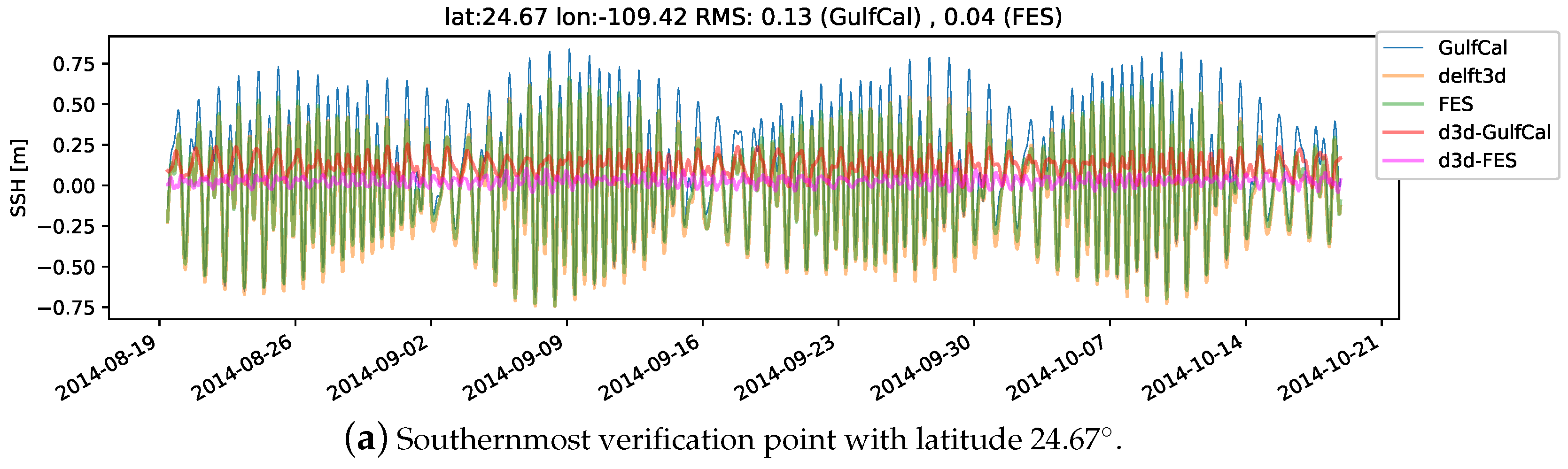
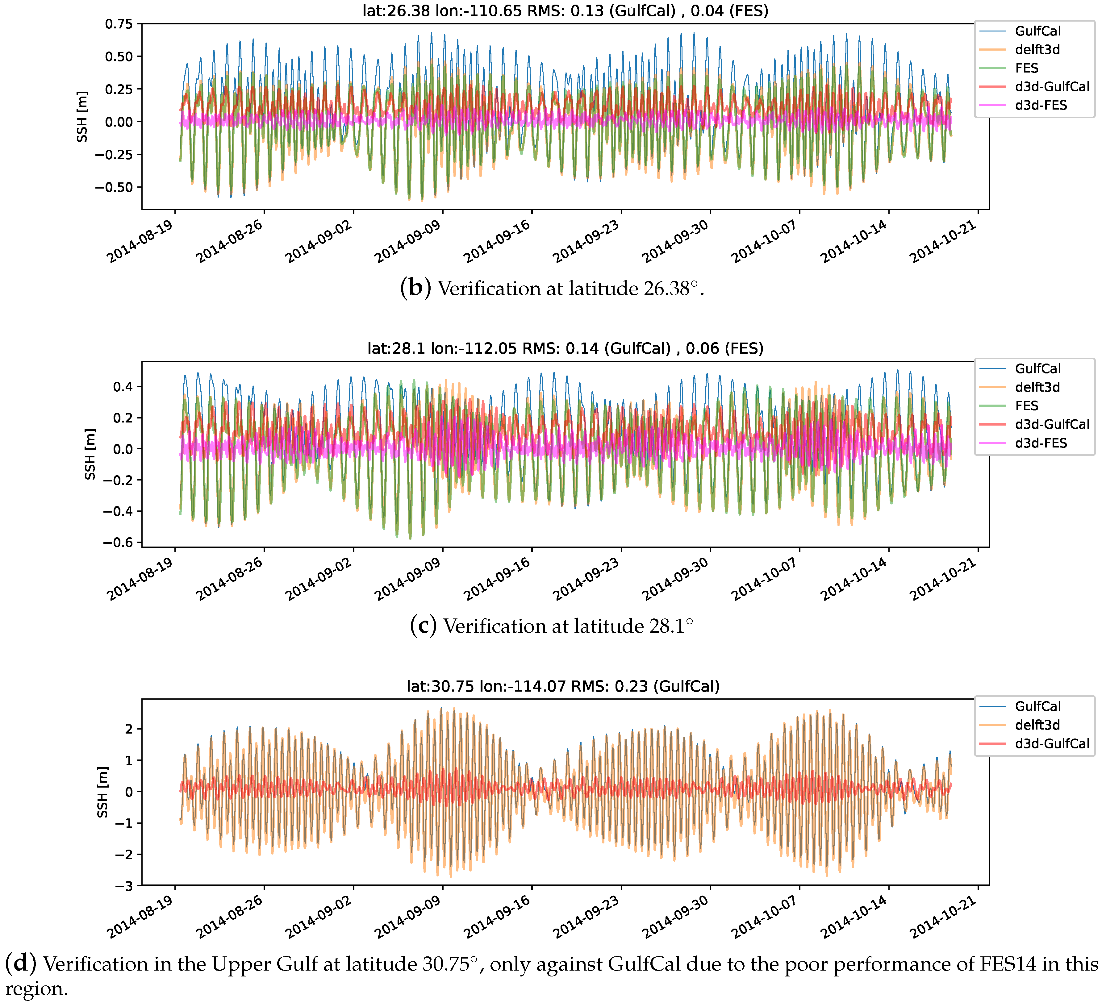
3.1. Sea Surface Height

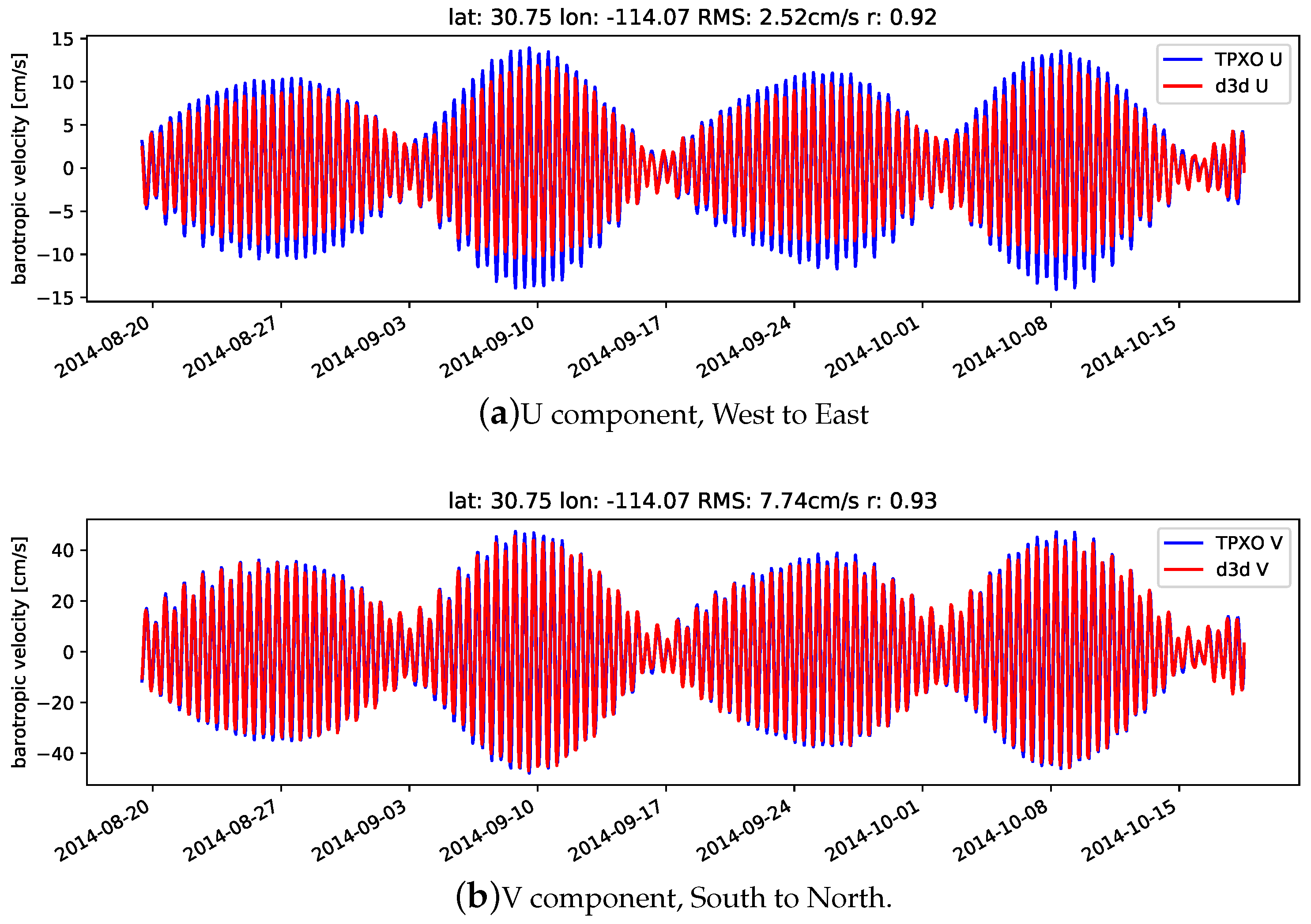
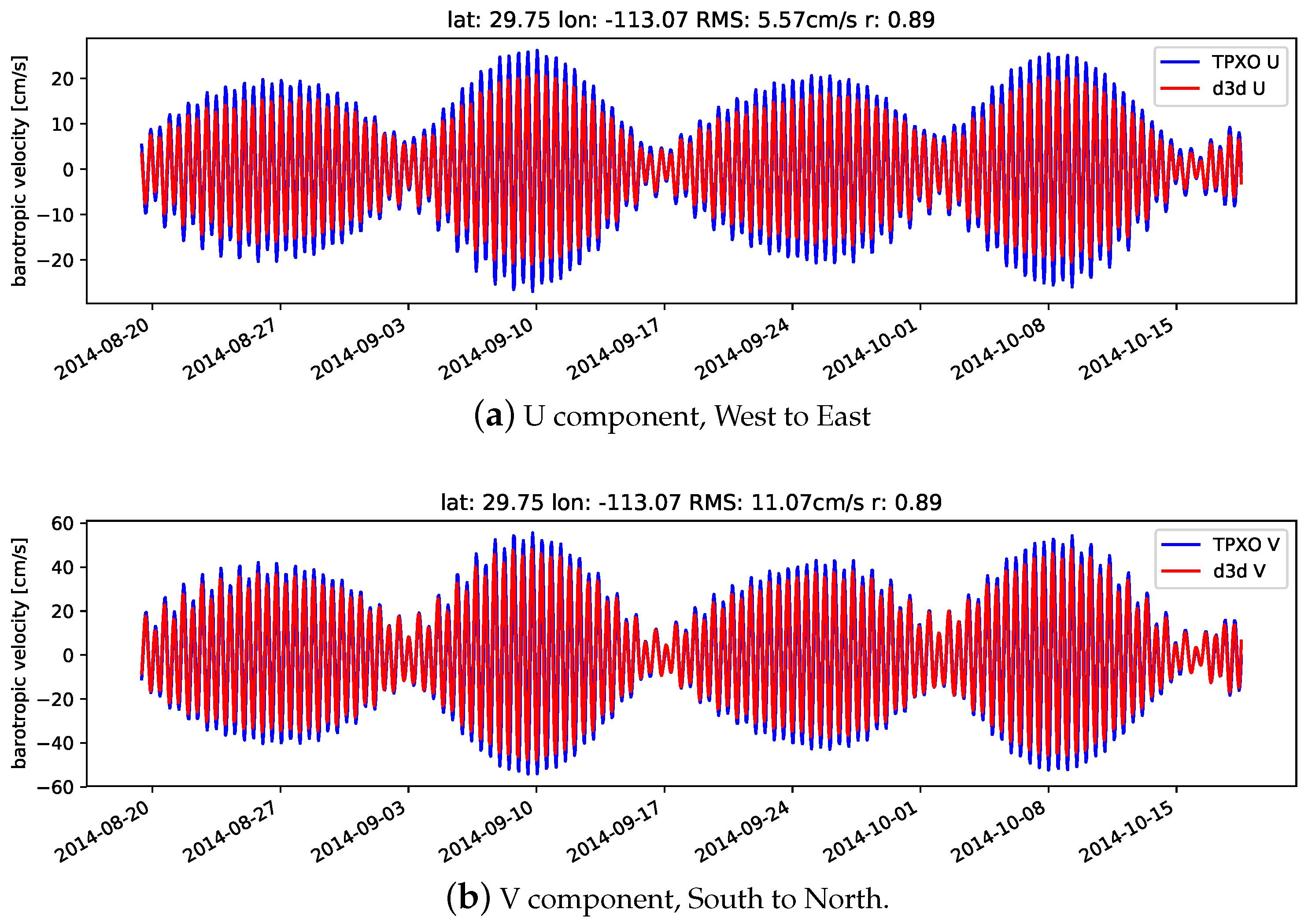
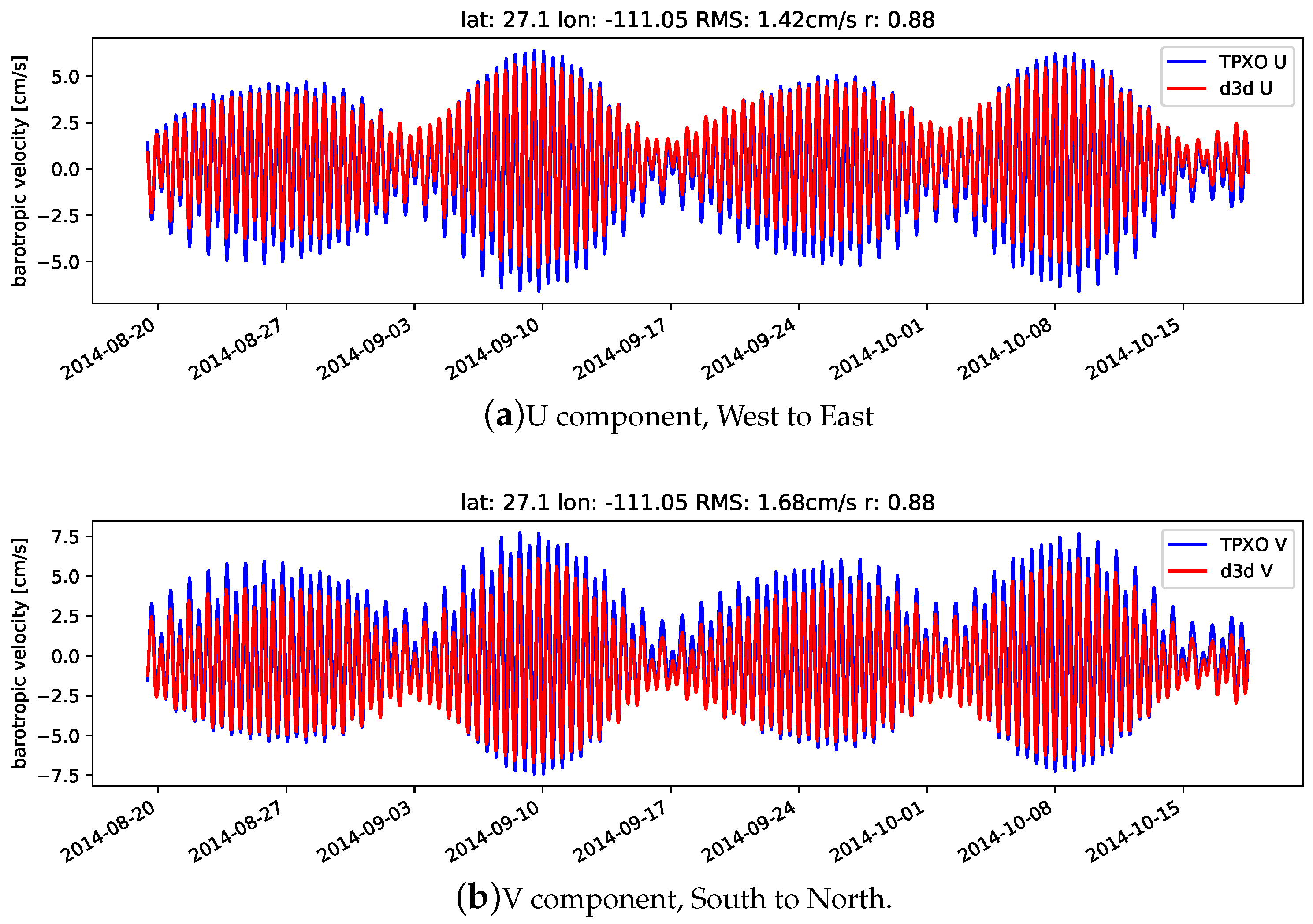
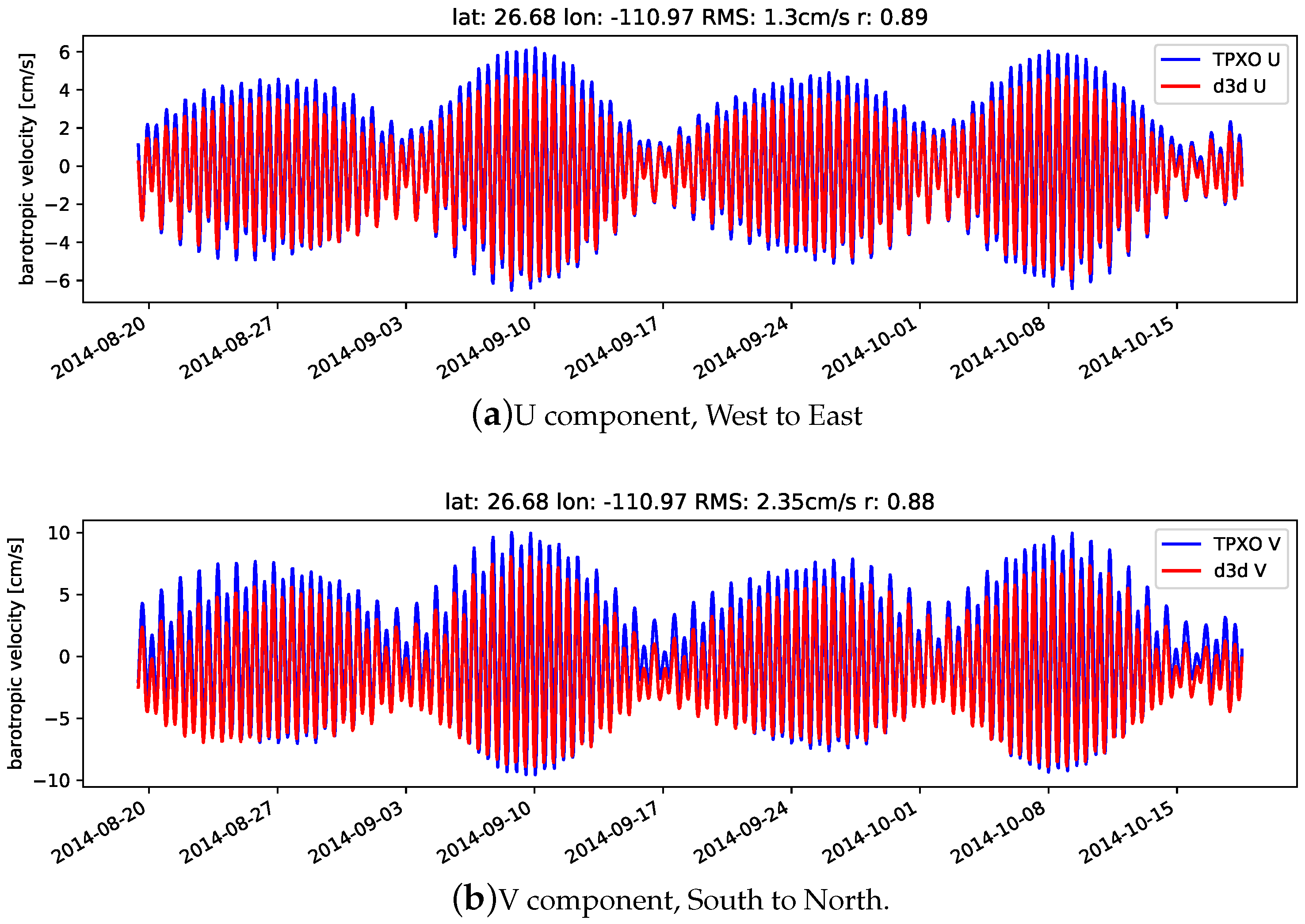
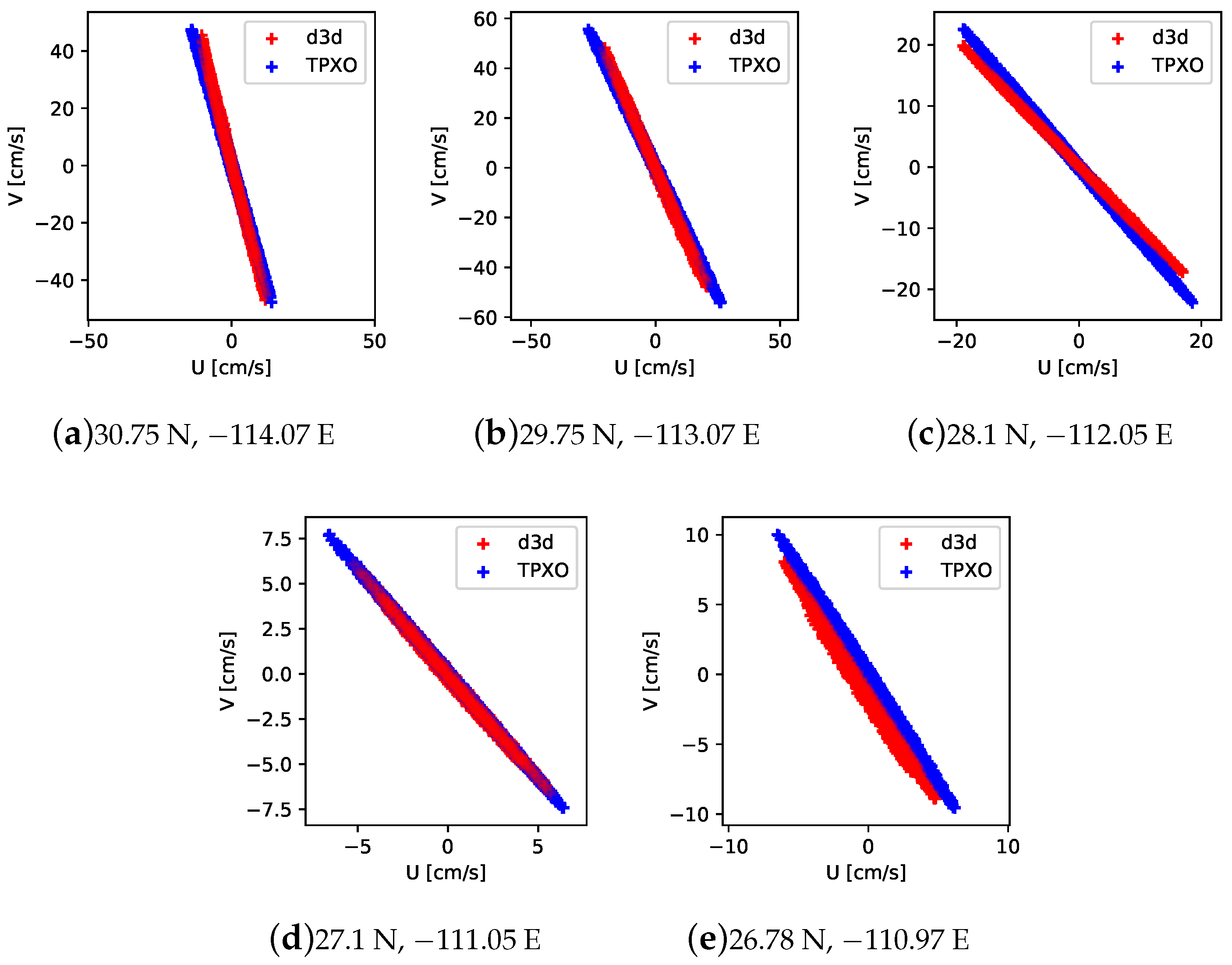
The model was verified against the FES (Finite Element Solution) 14 [35] in the lower Gulf. The FES14 tide model was developed during 2014–2016. The foundation of FES14 is a spectral tidal barotropic equation (T-UGO model). The global finite element grid contains 2.9 million nodes. The accuracy of the solution from the tidal model is improved through the assimilation of altimetry data provided by Topex/Poseidon, Jason-1, Jason-2, TPN-J1N, and ERS-1, ERS-2, ENVISAT, as well as tidal gauges. In the upper Gulf, where the FES14 solution is not reliable, the model was validated against GulfCal. The tide only Delft3d simulation with the highest vertical resolution was used for the verification. The RMS and Person-r values obtained are presented in

Table 1. Root mean square error (RMS) of sea surface height from GulfCal versus Delft3d, FES14 versus Delft3d, and the respective Pearson correlation coefficients, over the simulation period. The Pearson p are effectively zero for all cases. The first 250 h of the simulation were discarded to remove the spin-up.

Latitude	Longitude	RMS GulfCal-d3d [m]	RMS FES-d3d [m]	r GulfCal-d3d	r FES-d3d
30.73	−114.07	0.23	1.14	0.986	0.309
28.10	−112.04	0.14	0.06	0.919	0.959
26.36	−110.67	0.13	0.04	0.977	0.988
24.65	−109.42	0.13	0.04	0.990	0.996

.

Apart from the Upper Gulf, the correlation with FES14 is higher than the correlation with GulfCal. The RMS errors are small, 0.2m in the Upper Gulf, and 0.13 in the lower Gulf. In general, Delft3d is verifying better against FES14. In the Upper Gulf, GulfCal is validated against buoy observations and direct measurements, and, hence, is more reliable than the altimetry based model, FES. Therefore, the better validation of the presented model in the Upper Gulf against GulfCal is satisfying. In the lower Gulf, the coastline is sufficiently far away, allowing for accurate satellite observations. Here the results of the FES are good and understood to be more reliable than the GulfCal results. The time-series of sea surface height (SSH) are plotted in Figure 5.

3.2. Currents

Here, Delft3d is run as a barotropic model. Therefore, the currents have to be compared to the barotropic component of the observed currents. These have been obtained from the TPXO 8 atlas version 1 [33], using local solution SoC. All available constituents have been included, namely: m2, s2, n2, k2, k1, o1, p1, q1, m4, ms4, mn4, mm, and mf. The Delft3d solution has been depth-averaged for comparison with the TPXO currents, assuming piece-wise constant profiles over the sigma layers. West to East (U), and South to North (V) component time-series are compared in Figure 6, Figure 7, Figure 8, Figure 9 and Figure 10 for five points distributed along the Gulf, North to South. The tidal ellipses have been constructed from a scatter plot of the components and are shown in Figure 11 for the same five points.

The solutions, TPXO versus Delft3d, are generally in good agreement. The Pearson correlation in the Upper Gulf exceeds 0.9 for both components and the root mean square (RMS) errors are acceptable. Not surprisingly, the correlation drops towards the south of the Gulf, to 0.88. Here the deep sections, around 2000 to 3000 m, pose a challenge to the barotropic formulation.

The scatter plots of the velocity components of Delft3d and TPXO also agree, very well in orientation and well in magnitude, as was also apparent from the time-series plots.

4. Results

Resolving the surface forcing is vital in this study because, otherwise, the effects of the wind-driven shear stress on the rest of the water column will not be accurately reproduced. Therefore, ten separate experiments were conducted with increasing resolution of the surface layer. These tests will be described in more detail in the next section. With confidence in the vertical resolution, the data can then be analyzed for the anomaly and its spatial-temporal characteristics.

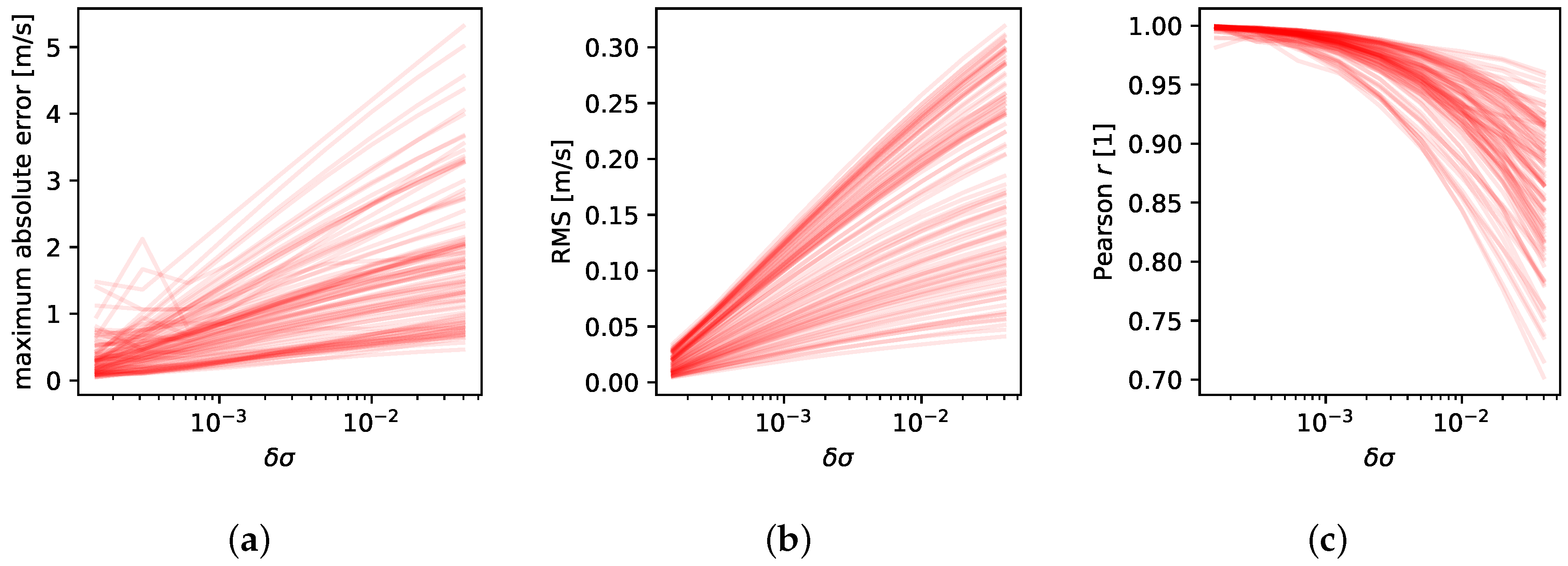
4.1. Convergence of the Wind Forcing with Vertical Resolution

The wind forcing is a surface-driven process. If the vertical resolution is not sufficient, then the velocities will not be accurately captured, that is, the mean across the sigma level is very different to the velocity at the top and bottom boundaries of the respective sigma level. The risk here is that only their mean effect on the top layer is resolved. In order to avoid this, the vertical resolution of the model was increased continuously until the surface velocities converged. First, a model with a grid of 25 layers with a uniform vertical resolution, resulting in a constant dimensionless layer thickness of 0.04, was run. Then, the first layer, with a thickness of 0.04, was replaced by two layers with a thickness of 0.02. Then, the top layer of 0.02 was replaced by two layers with thickness 0.01, down to the highest possible vertical resolution allowed by the model, corresponding to a layer with a thickness of $\Delta \sigma =0.0001$. This procedure yielded ten different vertical discretizations, listed in

Table 2. Vertical discretization for the ten convergence test runs. The thickness of each level is given in percent $\sigma$. In run 1, all 25 levels have 4% $\sigma$. In run 2, the first 24 levels have a thickness of 4% $\sigma$, the last two, level 25 and 26 2% $\sigma$ thick. Similar for the remaining runs. All values are rounded to three decimal places for presentation.

Vertical Level	run 1	run 2	…	run 7	run 8	run 9	run 10
34			…				0.010
33			…			0.016	0.010
32			…		0.031	0.016	0.020
31			…	0.063	0.031	0.031	0.040
30			…	0.063	0.063	0.062	0.080
29			…	0.125	0.125	0.125	0.160
28			…	0.250	0.250	0.250	0.320
27			…	0.500	0.500	0.500	0.640
26		2.0	…	1.000	1.000	1.000	1.280
25	4.0	2.0	…	2.000	2.000	2.000	1.440
24	4.0	4.0	…	4.000	4.000	4.000	4.000
…	…	…	…	…	…	…	…
1	4.0	4.0	…	4.000	4.000	4.000	4.000

. Note that the last column of that table does not follow this scheme precisely due to the minimum thickness of $0.01\%$ allowed by the model.

The velocity field of the surface (or first) sigma layer of run 10, that is, the experiment with $\Delta \sigma =0.0001$ was used as the reference value, or true value, and is denoted $v_{\delta {\sigma }_0=0.0001}$ in the following. With this reference value, a numerical convergence study was performed to demonstrate satisfactory convergence of the model result. Figure 12, shows a convergence of the Pearson r and RMS error below $0.05$ ms${}^{-1}$ for $\delta \sigma <2\times {10}^{-3}$, which is acceptable.

Subsequently, once it was ensured that the surface force was well resolved within the model (in terms of numerical convergence), the current anomaly due to the effect of the wind on the circulation could be assessed with confidence. The convergence with vertical resolution is presented in Figure 13.

Large errors are present in the models with coarse vertical grids near the surface. Only at $\delta {\sigma }_0=0.0025$ are most of the errors below $0.16$ ms${}^{-1}$.

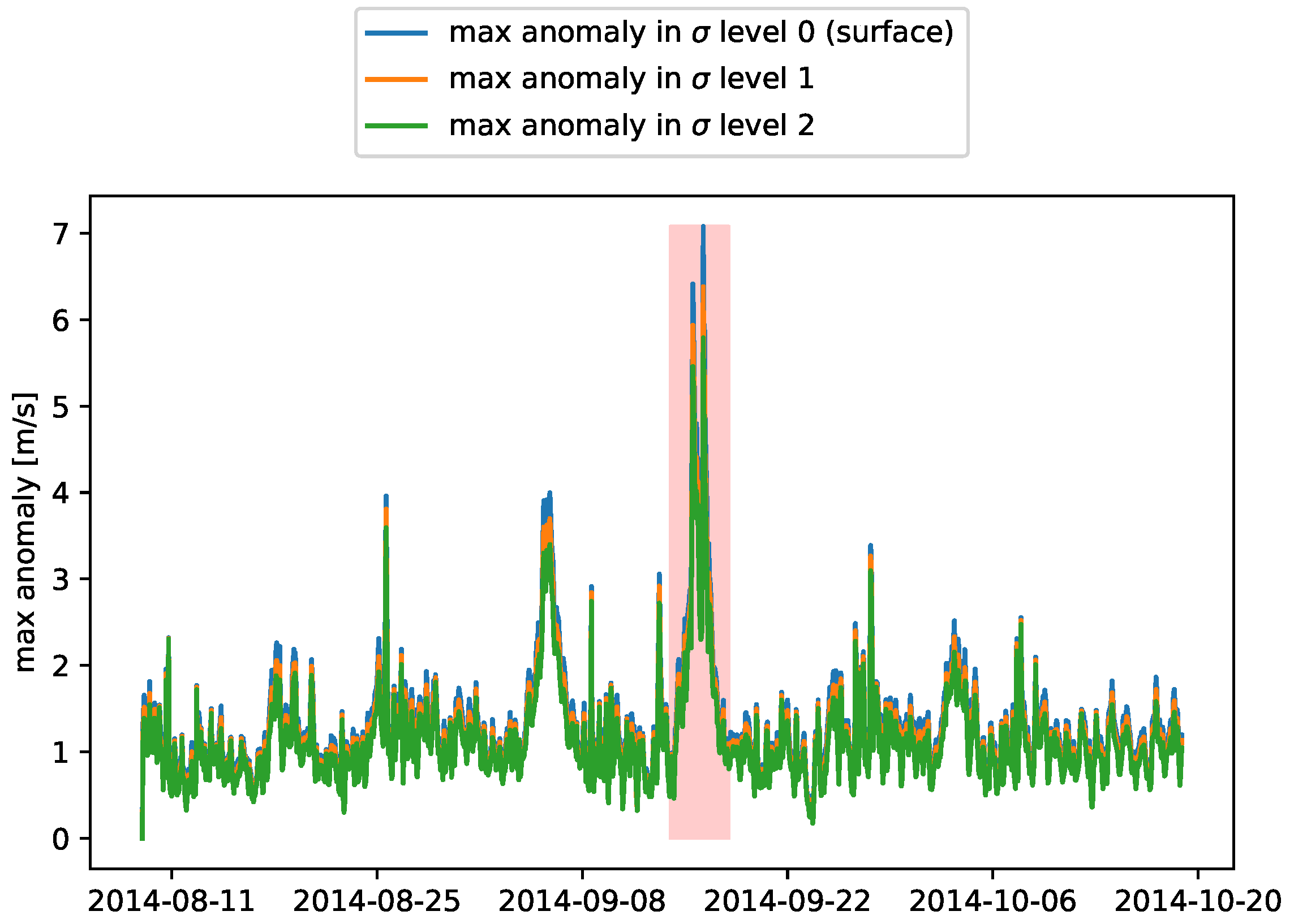
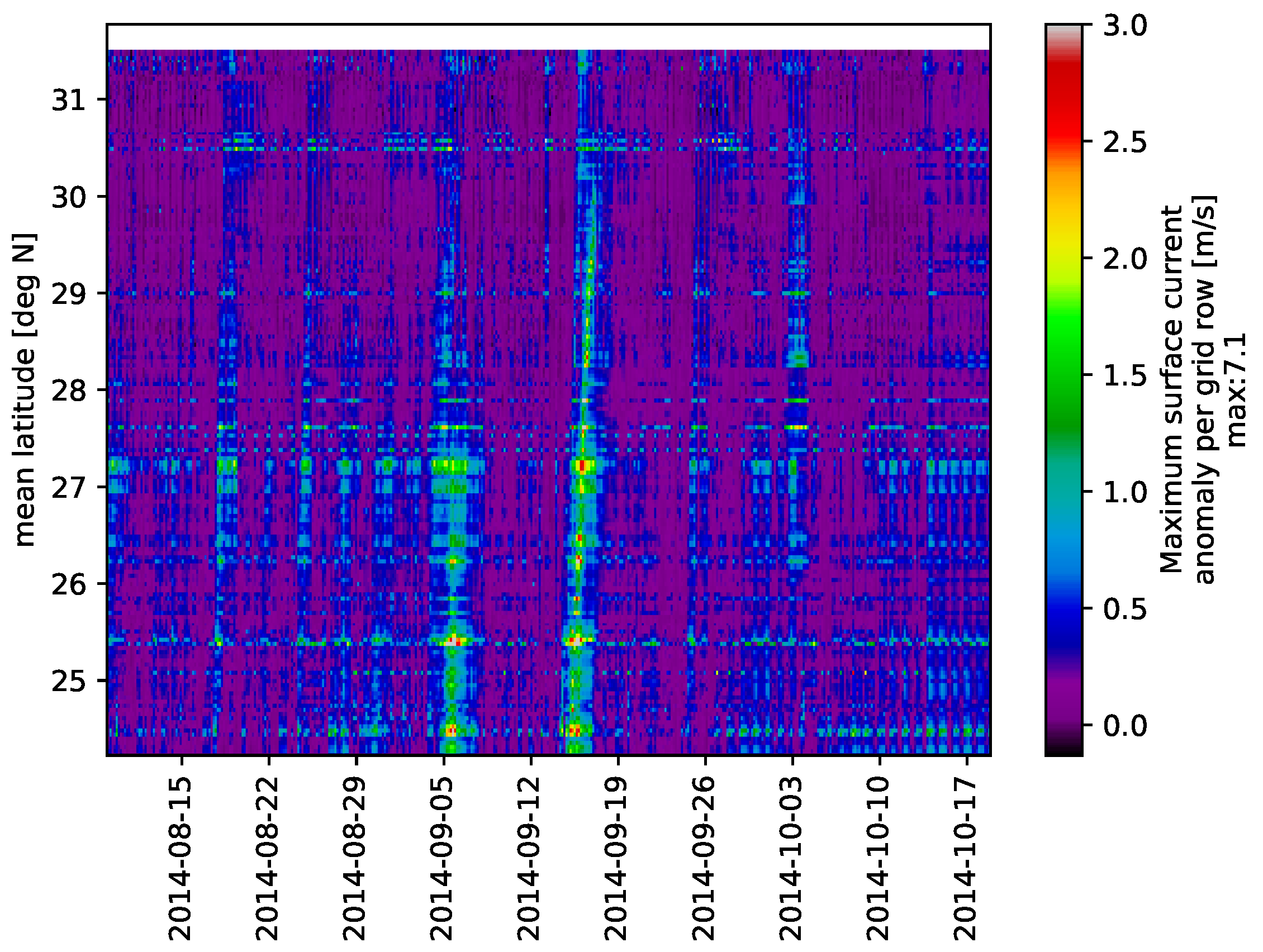
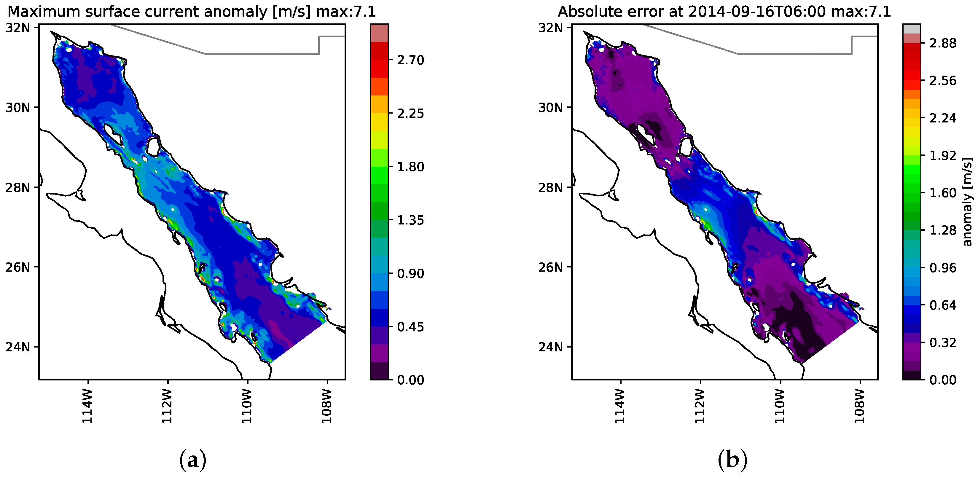
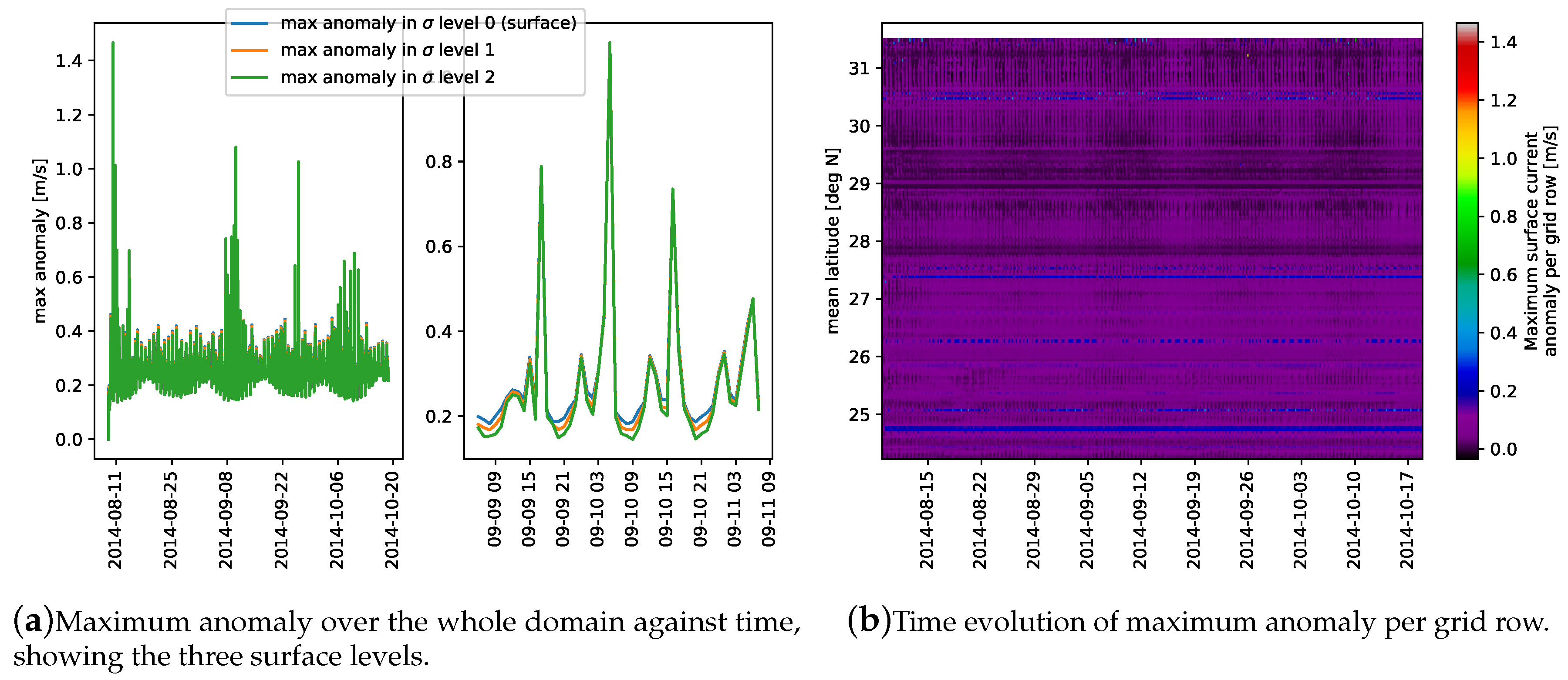
4.2. Maximum Anomaly in Surface Currents

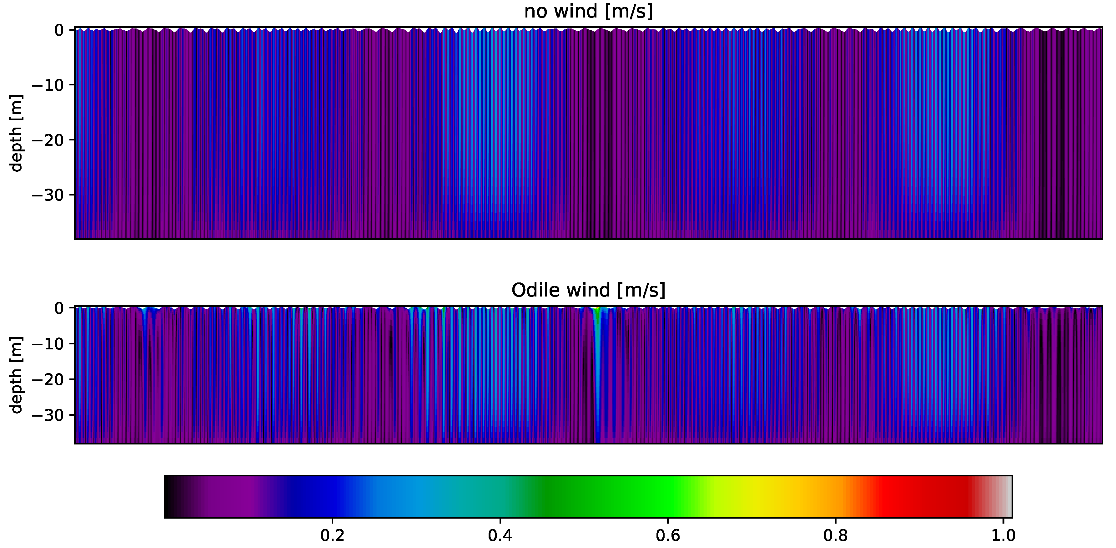
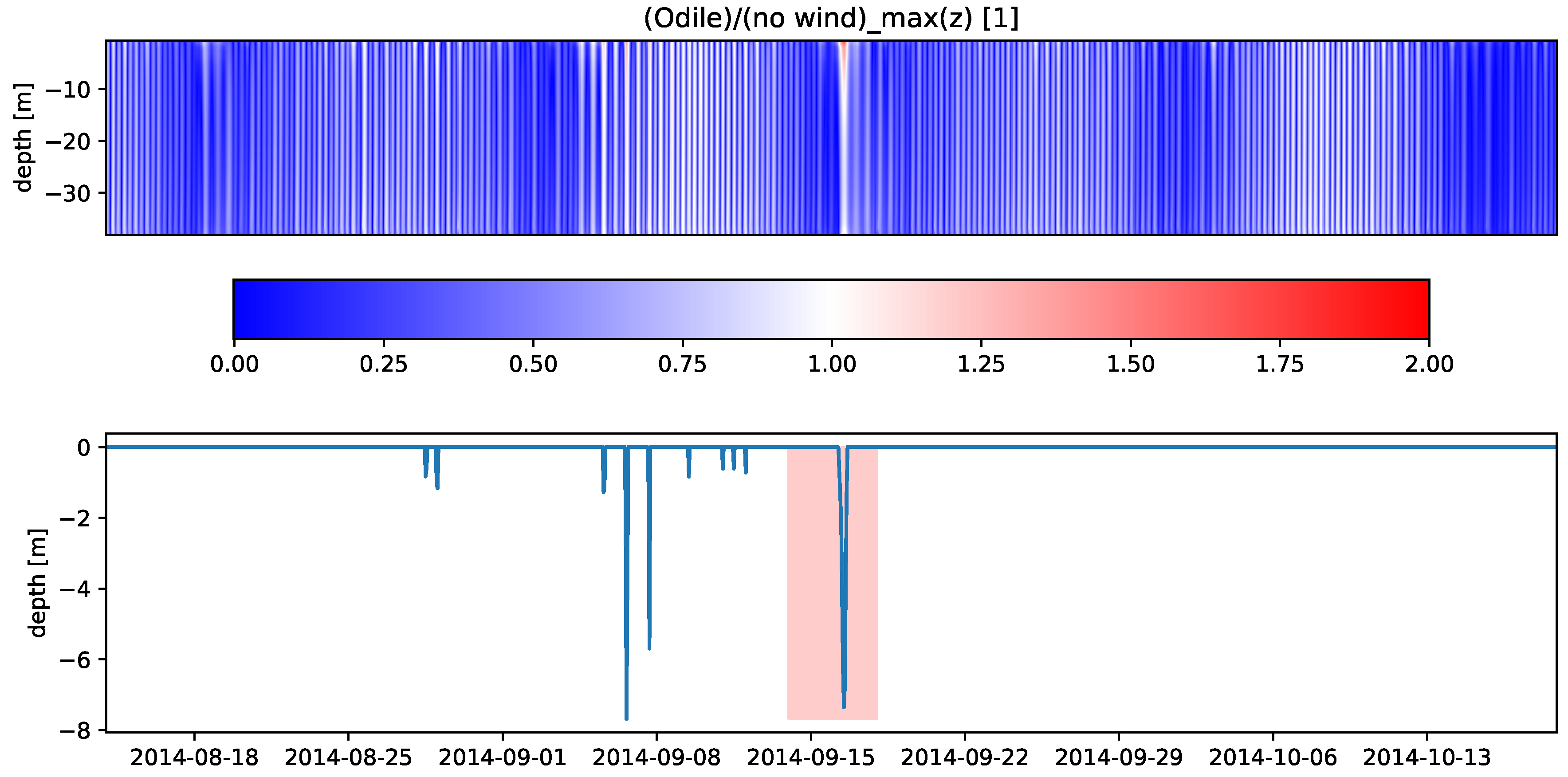
4.2.1. Comparison Odile—No Wind

The maximum surface current speed anomaly reaches 6 m/s. Figure 14 shows the time series of the maximum anomaly over the whole domain. The temporal evolution per grid row (West to East) is shown in Figure 15.

In that Figure, it can be seen that the 6 m/s values are isolated peaks, and for the largest part, the anomaly is between one and two meters per second. Plotting the maximum anomaly per grid point on a map of the Gulf, shown in Figure 16, shows that the most considerable impacts of the hurricane on the current speeds occur at the coast or close to islands. Due to techno-economic constraints, tidal energy converters (TECs) would also be installed near the coast (in shallow water) or close to islands, at least at the early stages of development [2]. Therefore, the probability of TEC damage due to the passage of the hurricane is great.

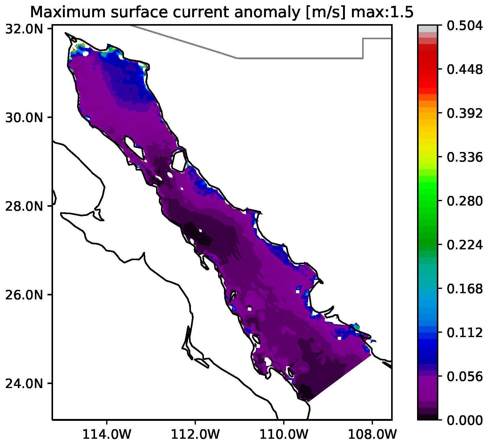
4.2.2. Wind Climatology Induced Surface Current Anomaly

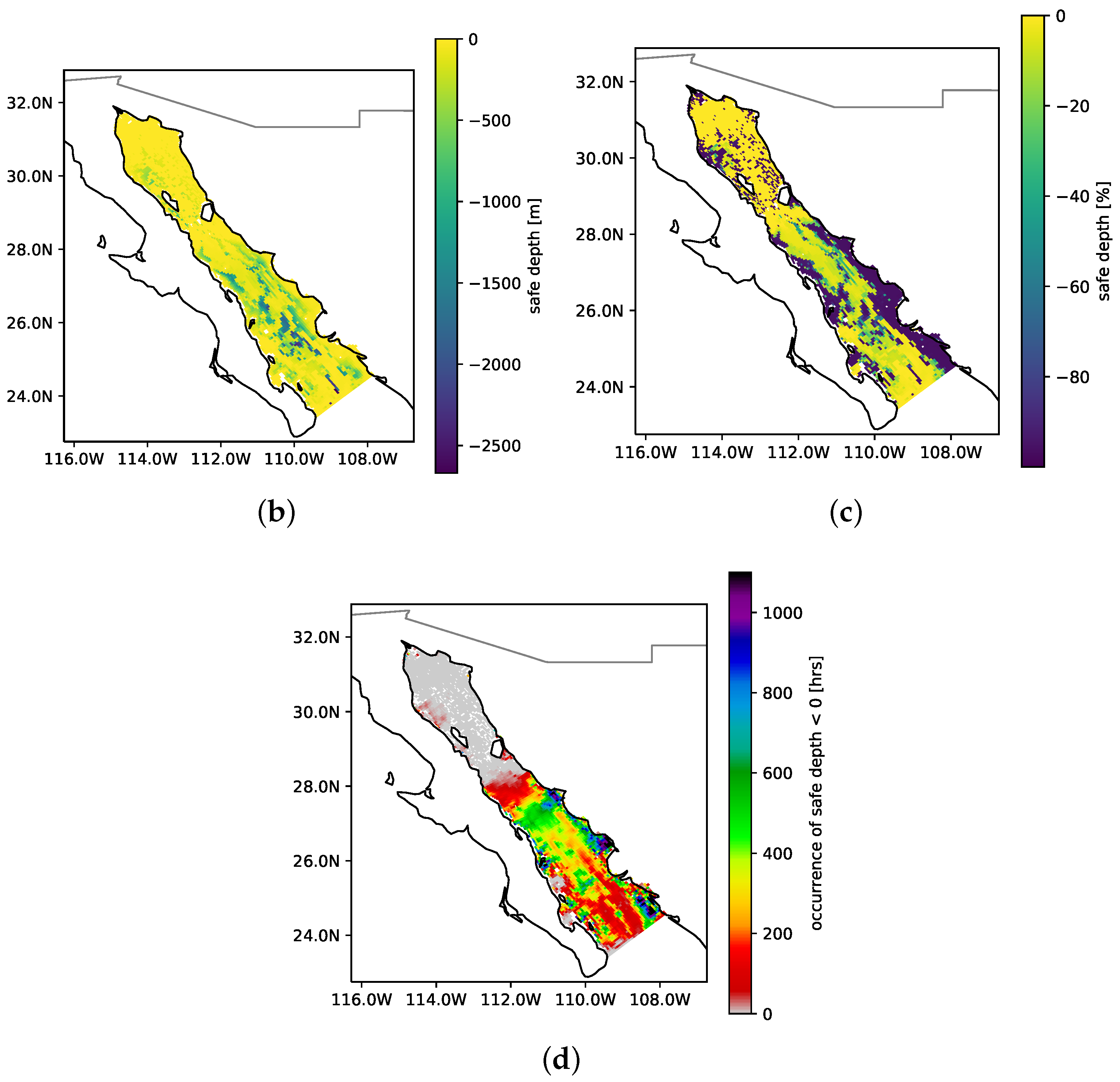
In contrast to the results presented for Odile above, the wind climate for September induces only moderate current anomalies of approximately 0.04 to 0.16 m/s, mainly at the East Coast and in shallow waters. A map of the anomaly is provided in Figure 17.

The recorded extremes of up to 1.4 m/s are only observed in isolated grid points or in extremely shallow areas, where the wind has an impact on the flooding and drying pattern. From this, it is clear that the strong winds during Odile have an impact several orders of magnitude larger than the climatology.

4.3. Safe Depth

The hurricane impact on renewable energy conversion can also be assessed in terms of “safe depth”. The safe depth is here introduced as the depth beyond which the currents observed during hurricane conditions are slower than an “assumed safe” current. “Safe depth” is a significant indicator of TEC survivability, in analogy to the cut-out speed of 25 m s${}^{-1}$ for commercial wind turbines [36]. Here, the assumed safe current is taken as 115% of the maximum current for the specific depth and location in the no-wind case. Hence, this formulation is depth-dependent. It assumes that the device installed at a certain depth is designed for the currents prevailing at this depth. Note that, nevertheless, this is a device–dependent value, and for a specific device, one may want to run a separate analysis.

Figure 18 shows the time series of currents without and with wind, in the top panel and the second from the top panel, respectively. The period over which Odile traveled along the Baja California Peninsula is highlighted in the bottom panel in red. A peak in the currents can be identified in the time-series. Peaks are also present from the minor storms and high wind episodes leading up to Odile.

5. Discussion

A clear signature of hurricane Odile and the storms before and after has been found in the analysis of the anomalies of the currents in the GC. Clear peaks in current anomaly are present in the time series, with anomalies of several meters per second, reaching anomaly maxima of up to 7.1 m/s. Most of these extreme values are to be found at coastal locations, and therefore damage to TEC devices caused by the passage of hurricanes has a high probability of occurrence. However, anomalies of 0.5 to 1.5 m/s can be found in large parts of the Gulf, as shown in Figure 16. The anomalies introduced by the wind climatology, Figure 17, are at least one order of magnitude lower, around 0.05 to 0.08 m/s, than the anomalies caused by Odile. Moreover, in coastal areas, the anomaly can penetrate to the seafloor, see Figure 19, therefore even bottom-mounted TEC devices may be affected by the passage of hurricanes, contrary to what has been previously assumed [37]. However, in large parts of the Gulf, the impact of the hurricane winds only penetrates around 5–30%. The temporal pattern of the anomaly shows a clear north-south divide: below 28${}^{\circ }$ N the anomaly exists for more than two days over the simulation period, but at latitudes above 28${}^{\circ }$ N the anomalies exists for substantially shorter periods. Therefore, one would expect that TEC devices operating at latitudes above 28${}^{\circ }$ N would suffer less damage than those operating below it. The probability of occurrence of category four hurricanes in the Gulf of California is larger below 28${}^{\circ }$ N than above it. Thus, in the first stages of development, the results indicated that one should install bottom-mounted devices above 28${}^{\circ }$ N and near the shore as per current devices specifications. However, taking seabed scour remedial actions and building TEC blades with materials that can withstand fatigue loads, as suggested by Reference [37], may still be necessary for TECs operating at such locations.

6. Conclusions

In this study, the impact of the extreme winds of hurricane Odile on the tidal currents in the Gulf of California has been evaluated. These results can inform site selection, and imply that device developers need to consider mitigation strategies to reduce the risk of damage to the device. This evaluation will help exploit the resource economically, safely and efficiently. From an academic perspective, the importance of wind-driven currents under hurricane conditions is a driver for further model developments, in aspects such as resolution and coverage of other hurricanes or high wind events. The analysis of the effect of the wind climatology on the coastal circulation may also be interesting from the diurnal cycle perspective. In particular, as the diurnal wind forcing cycle is in phase with the Coriolis frequency at these latitudes, interesting local effects can be expected.

References

1. Sinden, G.E. Renewable Electricity Generation: Resource Characteristics and Implications of Wind, Wave and Tidal Stream Power in the UK; Technical Report; UK Department of Energy and Climate Change: London, UK, 2007.
2. Roberts, A.; Thomas, B.; Sewell, P.; Khan, Z.; Balmain, S.; Gillman, J. Current tidal power technologies and their suitability for applications in coastal and marine areas. J. Ocean Eng. Mar. Energy 2016, 2, 227–245. [Google Scholar] [CrossRef] [Green Version]
3. Cresswell, N.; Ingram, G.; Dominy, R. The impact of diffuser augmentation on a tidal stream turbine. Ocean Eng. 2015, 108, 155–163. [Google Scholar] [CrossRef] [Green Version]
4. Segura, E.; Morales, R.; Somolinos, J. Cost Assessment Methodology and Economic Viability of Tidal Energy Projects. Energies 2017, 10, 1806. [Google Scholar] [CrossRef] [Green Version]
5. Haas, K.A.; Fritz, H.M.; French, S.P.; Smith, B.T.; Neary, V. Assessment of Energy Production Potential from Tidal Streams in the United States; Technical Report; Georgia Tech Research Corporation: Atlanta, GA, USA, 2011. [Google Scholar]
6. Rose, S.; Jaramillo, P.; Small, M.J.; Grossmann, I.; Apt, J. Quantifying the hurricane risk to offshore wind turbines. Proc. Natl. Acad. Sci. USA 2012, 109, 3247–3252. [Google Scholar] [CrossRef] [PubMed] [Green Version]
7. Black, W.J.; Dickey, T.D. Observations and analyses of upper ocean responses to tropical storms and hurricanes in the vicinity of Bermuda. J. Geophys. Res. 2008, 113, C08009. [Google Scholar] [CrossRef] [Green Version]
8. Hiriart Le Bert, G. Potencial energético del Alto Golfo de California. Boletín de la Sociedad Geológica Mexicana 2009, 61, 143–146. [Google Scholar] [CrossRef]
9. Carbajal, N.; Backhaus, J.O. Simulation of tides, residual flow and energy budget in the Gulf of California. Oceanol. Acta 1998, 21, 429–446. [Google Scholar] [CrossRef] [Green Version]
10. Romero-Vadillo, E.; Zaytsev, O.; Morales-Pérez, R. Tropical cyclone statistics in the Northeastern Pacific. Atmósfera 2007, 20, 197–213. [Google Scholar]
11. Cangialosi, J.P.; Kimberlain, T.B. Hurricane Odile (EP152014); Technical Report; National Hurricane Center: Miami, FL, USA, 2015. [Google Scholar]
12. Stelling, G.S. On the Construction of Computational Methods for Shallow Water Flow Problems. Ph.D. Thesis, Delft University of Technology, Delft, The Netherlands, 1983. [Google Scholar]
13. Lavín, M.F.; Marinone, S.G. An Overview of the Physical Oceanography of the Gulf of California. In Nonlinear Processes in Geophysical Fluid Dynamics; Springer: Berlin/Heidelberg, Germany, 2003; pp. 173–204. [Google Scholar] [CrossRef] [Green Version]
14. Phillips, N.A. A Coordinate System having some special advantages for numerical forecasting. J. Meteorol. 1957, 14, 184–185. [Google Scholar] [CrossRef] [Green Version]
15. Deltares. Delft3D-FLOW User Manual Version 3.15: Simulation of Multi-Dimensional Hydrodynamic Flows and Transport Phenomena, Including Sediments; Technical Report; Deltares: Delft, The Netherlands, 2018. [Google Scholar]
16. Bryant, K.; Akbar, M. An Exploration of Wind Stress Calculation Techniques in Hurricane Storm Surge Modeling. J. Mar. Sci. Eng. 2016, 4, 58. [Google Scholar] [CrossRef]
17. Akbar, M.; Kanjanda, S.; Musinguzi, A. Effect of Bottom Friction, Wind Drag Coefficient, and Meteorological Forcing in Hindcast of Hurricane Rita Storm Surge Using SWAN +ADCIRC Model. J. Mar. Sci. Eng. 2017, 5, 38. [Google Scholar] [CrossRef] [Green Version]
18. Zhao, Z.K.; Liu, C.X.; Li, Q.; Dai, G.F.; Song, Q.T.; Lv, W.H. Typhoon air-sea drag coefficient in coastal regions. J. Geophys. Res. Oceans 2015, 120, 716–727. [Google Scholar] [CrossRef]
19. Bordoni, S.; Ciesielski, P.E.; Johnson, R.H.; McNoldy, B.D.; Stevens, B. The low-level circulation of the North American Monsoon as revealed by QuikSCAT. Geophys. Res. Lett. 2004, 31, L10109. [Google Scholar] [CrossRef] [Green Version]
20. Badan-Dangon, A.; Dorman, C.E.; Merrifield, M.A.; Winant, C.D. The lower atmosphere over the Gulf of California. J. Geophys. Res. 1991, 96, 16877. [Google Scholar] [CrossRef]
21. Douglas, M.W. The Summertime Low-Level Jet over the Gulf of California. Mon. Weather Rev. 1995, 123, 2334–2347. [Google Scholar] [CrossRef] [Green Version]
22. Mizielinski, M.S.; Roberts, M.J.; Vidale, P.L.; Schiemann, R.; Demory, M.E.; Strachan, J.; Edwards, T.; Stephens, A.; Lawrence, B.N.; Pritchard, M.; et al. High-resolution global climate modelling: The UPSCALE project, a large-simulation campaign. Geosci. Mod. Dev. 2014, 7, 1629–1640. [Google Scholar] [CrossRef] [Green Version]
23. Donlon, C.J.; Martin, M.; Stark, J.; Roberts-Jones, J.; Fiedler, E.; Wimmer, W. The Operational Sea Surface Temperature and Sea Ice Analysis (OSTIA) system. Remote Sens. Environ. 2012, 116, 140–158. [Google Scholar] [CrossRef]
24. Walters, D.N.; Best, M.J.; Bushell, A.C.; Copsey, D.; Edwards, J.M.; Falloon, P.D.; Harris, C.M.; Lock, A.P.; Manners, J.C.; Morcrette, C.J.; et al. The Met Office Unified Model Global Atmosphere 3.0/3.1 and JULES Global Land 3.0/3.1 configurations. Geosci. Mod. Dev. 2011, 4, 919–941. [Google Scholar] [CrossRef] [Green Version]
25. Black, T.L. The New NMC Mesoscale Eta Model: Description and Forecast Examples. Weather Forecast. 1994, 9, 265–278. [Google Scholar] [CrossRef] [Green Version]
26. Mesinger, F.; DiMego, G.; Kalnay, E.; Mitchell, K.; Shafran, P.C.; Ebisuzaki, W.; Jović, D.; Woollen, J.; Rogers, E.; Berbery, E.H.; et al. North American Regional Reanalysis. Bull. Am. Meteorol. Soc. 2006, 87, 343–360. [Google Scholar] [CrossRef] [Green Version]
27. Kanamitsu, M.; Ebisuzaki, W.; Woollen, J.; Yang, S.K.; Hnilo, J.J.; Fiorino, M.; Potter, G.L. NCEP–DOE AMIP-II Reanalysis (R-2). Bull. Am. Meteorol. Soc. 2002, 83, 1631–1644. [Google Scholar] [CrossRef]
28. Atlas, R.; Hoffman, R.N.; Bloom, S.C.; Jusem, J.C.; Ardizzone, J. A Multiyear Global Surface Wind Velocity Dataset Using SSM/I Wind Observations. Bull. Am. Meteorol. Soc. 1996, 77, 869–882. [Google Scholar] [CrossRef] [Green Version]
29. Atlas, R.; Hoffman, R.N.; Ardizzone, J.; Leidner, S.M.; Jusem, J.C.; Smith, D.K.; Gombos, D. A Cross-calibrated, Multiplatform Ocean Surface Wind Velocity Product for Meteorological and Oceanographic Applications. Bull. Am. Meteorol. Soc. 2011, 92, 157–174. [Google Scholar] [CrossRef]
30. Hoffman, R.N.; Leidner, S.M.; Henderson, J.M.; Atlas, R.; Ardizzone, J.V.; Bloom, S.C. A Two-Dimensional Variational Analysis Method for NSCAT Ambiguity Removal: Methodology, Sensitivity, and Tuning. J. Atmos. Ocean. Technol. 2003, 20, 585–605. [Google Scholar] [CrossRef]
31. Saha, S.; Moorthi, S.; Pan, H.L.; Wu, X.; Wang, J.; Nadiga, S.; Tripp, P.; Kistler, R.; Woollen, J.; Behringer, D.; et al. The NCEP Climate Forecast System Reanalysis. Bull. Am. Meteorol. Soc. 2010, 91, 1015–1058. [Google Scholar] [CrossRef]
32. Bentamy, A.; Fillon, D.C. Gridded surface wind fields from Metop/ASCAT measurements. Int. J. Remote Sens. 2011, 33, 1729–1754. [Google Scholar] [CrossRef] [Green Version]
33. Egbert, G.D.; Erofeeva, S.Y. Efficient Inverse Modeling of Barotropic Ocean Tides. J. Atmos. Ocean. Technol. 2002, 19, 183–204. [Google Scholar] [CrossRef] [Green Version]
34. Marinone, S.; González, J.; Figueroa, J. Prediction of currents and sea surface elevation in the Gulf of California from tidal to seasonal scales. Environ. Mod. Softw. 2009, 24, 140–143. [Google Scholar] [CrossRef]
35. FES2014 Was Produced by Noveltis, Legos and CLS and Distributed by Aviso+, with Support from CNES. Available online: https://www.aviso.altimetry.fr/ (accessed on 2 August 2019).
36. Khare, V.; Khare, C.; Nema, S.; Baredar, P. Tidal Energy Systems: Design, Optimization and Control; Elsevier: Amsterdam, The Netherlands, 2018. [Google Scholar]
37. Chen, L.; Lam, W.H. A review of survivability and remedial actions of tidal current turbines. Renew. Sustain. Energy Rev. 2015, 43, 891–900. [Google Scholar] [CrossRef] [Green Version]
Figure 1. Computational grid with variable resolution. In the cross-Gulf direction the resolution varies from 2.55 km to 5.621 km and in the long-Gulf direction from 3.073 km to 6.465 km.
Jmse 08 00080 g001
Figure 2. Wind field during Hurricane Odile. The HURDAT trajectory (see https://www.aoml.noaa.gov/hrd/data_sub/hurdat.html) is shown as a dark blue line, wind vectors as black quivers and streamlines as light blue lines. All times in UTC. The geographical position of Odile is indicated.
Jmse 08 00080 g002
Figure 3. Wind field climatologies.
Jmse 08 00080 g003
Figure 4. Sources of wind climatology data and temporal coverage.
Jmse 08 00080 g004
Figure 5. Model verification against sea surface height (SSH) from GulfCal and FES14. Difference plots are indicated in the legend as “diff”. All dates in UTC.
Jmse 08 00080 g005aJmse 08 00080 g005b
Figure 6. Time-series of components of the barotropic current at latitude 30.75 N, longitude—114.07 E. The delf3D (d3d) components have been depth averaged for comparison. All dates in UTC.
Jmse 08 00080 g006
Figure 7. Time-series of components of the barotropic current at latitude 29.75 N, longitude—113.07 E. The delf3D (d3d) components have been depth-averaged for comparison. All dates in UTC.
Jmse 08 00080 g007
Figure 8. Time-series of components of the barotropic current at latitude 28.1 N, longitude—112.05 E. The delf3D (d3d) components have been depth-averaged for comparison. All dates in UTC.
Jmse 08 00080 g008
Figure 9. Time-series of components of the barotropic current at latitude 27.1 N, longitude—111.05 E. The delf3D (d3d) components have been depth-averaged for comparison. All dates in UTC.
Jmse 08 00080 g009
Figure 10. Time-series of components of the barotropic current at latitude 26.78 N, longitude—110.97 E. The delf3D (d3d) components have been depth-averaged for comparison. All dates in UTC.
Jmse 08 00080 g010
Figure 11. Scatter plot of U versus V components of the barotropic currents.
Jmse 08 00080 g011
Figure 12. Convergence analysis over the whole domain for the period of hurricane Odile, 14 September 2014–18 September 2014. (a) Maximum absolute velocity error, e r r = | v v δ σ 0 = 0.0001 | , (b) root mean square error, R M S = 1 / N e r r 2 , with N denoting the grid points with an initial depth of more than 3m, and (c) Pearson correlation coefficient, r.
Jmse 08 00080 g012
Figure 13. Maps of absolute error, e r r = | v δ σ 0 = n v δ σ 0 = 0.0001 | , with n denoting the vertical layer thickness in the surface layer at plot time step 912, 38 days after simulation start, 2014-09-16T00:00 UTC.
Jmse 08 00080 g013
Figure 14. Maximum surface current anomaly time series for the three topmost model layers. All dates in UTC.
Jmse 08 00080 g014
Figure 15. Maximum anomaly per grid row versus time. All dates in UTC.
Jmse 08 00080 g015
Figure 16. Current anomalies due to Odile. All times in UTC. (a) Map of maximum anomaly during simulation period for each grid point. (b) Map of the anomaly at the time of the maximum anomaly in the time series (c.f. Figure 14).
Jmse 08 00080 g016
Figure 17. Surface current anomalies due to climatological winds. All dates in UTC.
Jmse 08 00080 g017aJmse 08 00080 g017b
Figure 18. Safe depth at lat = 28.260 N lon = −111.772 W. Safe depth is here defined as the depth where the velocity never exceeds 1.15 v m a x ( z ) , the maximum velocity in the no-wind simulation, during the period starting at day five and finishing at the end of the simulation. The red rectangle indicates the period of Odile. The top two panels show the velocity profiles without and with Odile winds. The third panel from the top shows the velocity profile with Odile winds, normalised by the maximum velocity observed for the no wind case at the respective depth, therefore, showing a representation of safe depth before the restriction to a certain assumed safe current. The bottom panel shows the iso-line of the assumed safe current of 115%, as per the definition of the safe depth. All dates in UTC.
Jmse 08 00080 g018aJmse 08 00080 g018b
Figure 19. Safe depth analysis over the course of Hurricane Odile. (a) Safe depth in meters. (b) Percent of total depth, indicating locations where the anomaly extends through the whole water column. (c) Accumulated hours of occurrence of safe depth < 0, that is, duration of potential exposure of devices.
Jmse 08 00080 g019