Long-Term Stochastic Modeling of Sheet Pile Corrosion in Coastal Environment from On-Site Measurements

Abstract

Optimization of maintenance and design of coastal steel infrastructure needs for long-term predictive degradation models. The phenomenon of corrosion in the offshore and coastal environment is very complex due to the stochastic and changing nature of the environment (temperature, water chemical properties) and the multiple involved processes in competition. In the GEROM French project, the objective was to build a database of the residual thickness measured from ultrasonic measurements on sheet piles and piles carried out during 40 years in commercial and military harbors along the French coast. A total amount of 35,460 measurements were gathered. After a detailed analysis of the data and statistical modeling, a probabilistic model of corrosion is proposed for sheet piles. It relies on a piecewise description of the process with the depth depending on the exposed zone and a time-dependent evolution of parameters of the gamma probability density function.

1. Introduction

Corrosion of steel fixed or moving marine structures has focused attention on research since the beginning of the last century. It was required to design ships, piles, sheet piles by adding sacrificial thickness or by computing the required cathodic protection. The available models until now are of various forms and take more and more of a probabilistic form to account for uncertainties. Two types of uncertain outputs are proposed: the residual thickness (or the corroded thickness) and the corrosion rate. The latter requires an assumption of the evolution of the rate of time. For engineering purposes, the design lifetime is fixed and known; an average corrosion rate along the life-time is, therefore, usually provided. By focusing on inspection and maintenance optimization, the decision time (inspection/repair) is varying and a time-variant model of the residual thickness is needed.

Among the literature, one can classify the time-variant model of the loss of thickness in the marine environment, which is called “corrosion models” in the following four categories.

(i) Pure mathematical multi-linear models: they rely on the assumption that the corrosion rate is constant with time; herein a linear evolution of the loss of thickness (LoT) is assumed [1]. Melchers [2] extended these models to bi-linear and tri-linear [3] ones with a power law for modeling the evolution of mean and standard deviation with time. Paik et al. [4] expanded these models in a probabilistic way by modeling parameters as random variables. These models have been shown to be very conservative [3,5] and non-adaptive for the coastal environment where a constant value is achieved between 10 and 20 years [6]. Moreover, only the two first statistical moments were provided (mean and variance) and no probabilistic density function (pdf) was suggested.

(ii) Physical-chemical analytical models: developed by Chernov and Ponomarenko [7], the key idea is to introduce the protection property of the corrosion product and long term corrosion velocity as implicit parameters. These models were calibrated in several sites from corrosion analysis of coupons, but this model was not extended to a probabilistic one because of its mathematical expression (product and exponential) that is less adaptive for uncertainty transfers [8].

(iii) Pure mathematical exponential models: developed initially by Guedes Soares and Garbatov [4], Paik and Thayamballi [9,10], Qin and Cui [11], their difference relies mainly on the calibration method. Jonbloed et al. developed long-term (50 years) deterministic curves from corrosion measurement in the harbors of Rotterdam [12].

(iv) Phenomenological models: developed by Melchers et al. [13,14,15,16,17], their objective is to propose a versatile form that contains the uncertainty and the trends, and with four phases, the effect of bio-corrosion. The model is versatile but does not suggest, in its last form, the underlying pdf of the residual thickness.

During the last two decades, quite a lot of theoretical developments both on the modeling and the calibration were performed, mainly in the deterministic context. These models were rarely calibrated in the coastal environment and never with long-term data and a large database for statistical modeling.

Starting from these limitations and from several large inspection campaigns performed during the last three decades in some French harbors, the MEDACHS framework (Marine Environment Damage to Atlantic Coast Historical and transport works or Structures-Interreg IIIB Project funded by the EC 2005–2007) and after that the GEROM project (2005–2009) [18,19], developed a program of on-site data collection. The objective was to collect data from existing residual thickness measurements carried out in the four biggest harbors in France where the context (environmental) was recorded. Only uniform corrosion was analyzed here to develop a model required for structural reliability of sheet piles where pitting plays a secondary role. The amount of data was more than 1000 per structure per inspection and allowed statistical analysis of the LoT according to the different exposure areas (mainly tidal and immersion areas). In addition, the physico-chemical parameters (temperature, pH, oxygen, salinity, conductivity, nutrients) have been measured regularly since the early 2000s. After three years of the project, 35,460 points of measurements were collected in all exposure zones and for several harbor types. The objective is to perform complete statistical modeling, to introduce spatial modeling of the corrosion and a long-term corrosion model for sheet piles.

The paper is organized as follows. Section 2 presents the database. Firstly it outlines the protocol of measurement used in France which is used in this paper for residual thickness measurements. Secondly, it describes the whole database of 35,460 measurements both from structural and environmental points of view. Then, statistical analysis is carried out introducing the depth corrosion model. Section 3 presents the parameterization of the piecewise model of the corrosion process and the selection of gamma pdf for the fitting distribution of experimental data. The evolution of parameters of gamma pdf with time is fitted on the database and models for the time-dependence of the process. Section 4 concludes the paper and highlights the potential of the model for maintenance optimization and Bayesian updating.

2. Materials and Methods

2.1. Corrosion Database from On-Site Measurements in France

Ultrasonic non-destructive testing (NDT) classically assesses the corrosion of steel structures. The protocol associated with this NDT tool is recommended in France by the CETMEF (French Center for Maritime and Fluvial Technical Studies: Engineering Center of the French Ministry of Public Works, now CEREMA) [20]. It is usually followed by the owners and implemented by companies that carry out inspections of coastal steel structures. After calibration of the sensor, one of the key steps is the first one: the corrosion products are removed by grinding. This technique, and considering the harsh conditions (visibility, current, wake, …) for marine inspections, generates errors of measurements at each location of measurement. The error comes from both the physical measurement (around 0.1 mm) and the protocol (grinding, link diver-operator, etc. [20]). Thus, three measurements are carried out at a given location: the three measurements are distributed on a circle, with a diameter of about 5 cm, every 120° as shown in Figure 1. Our EuroMarCor database gathers 99,700 data. The average of these three readings is considered as the “true” loss of thickness (LoT) and is considered in the following for the modeling of LoT. Then the reduced number of data used in the following is 35,460. Note that we focus here on data concerning uniform corrosion on non-protected (cathodic or painting) structures. For on-pile wharves, with a view to analyzing the corrosion around the pile, measurements are carried out at several cardinal positions around the pile's section (see Figure 1). For wharves with an on-sheet pile-wall, they are performed along the length of the wharf about every 10 m, which is classically the mean distance between two piles for on-pile wharves. The reading of Ultrasonic NDT is a residual thickness value. Knowing the initial thickness of piles or sheet piles, we deduce the LoT mainly due to corrosion. Knowledge of the initial thickness can be an issue. For piles, the thickness of the ‘as-built’ pile could depend on the availability of non-compliant pile-lines for oil or gas transport. The change, if conservative, is not always reported in the construction documents. Unlike piles, the sheet piles’ thickness is not changed from the design documents. Our study focuses on the corrosion of sheet piles and the thickness used is the value reported in the design documents. The paper focuses on sheet piles and it does not require this measurement. Note that for U-shape sheet piles (like the HA7d wharf in the following), we focus in this paper only on the central part of the corrosion in the out-pan area. This area is more affected than the in-pan area due to oxygenation by the current and abrasion by solid particles in the water [20,21].

2.2. Type and Age of Considered Dock Structures

Corrosion measurements were collected on two types of marine structures: on pile wharves and on sheet pile wharves. This paper focuses on sheet piles only. Structures are located on all the French metropolitan coasts, i.e., Atlantic, Channel, and Mediterranean coasts.

Almost all the studied structures were built between 1955 and 1985. Only three structures are older than 1955 and none are more recent than 1985. The owners began NDT measurements of residual thicknesses from 1990. Consequently, most of the structures were 10 to 40 years old at the inspection time. Figure 2 presents the distribution of the age of the structures at the first, second, and third inspection times.

We focus on four harbors, called BO, HA, PL, and SE in the following. The distribution of the structures within the studied harbors according to the type of water variation (dock at constant sea-water level, wet dock and tidal dock) is presented in Figure 3.

Over a total of 23 structures, 11 are located in docks at constant seawater level, nine in tidal docks and three in wet docks. In this last case, the seawater level changes with the same period as the tide but with a lower amplitude. The maximum variation of the seawater level in the various docks is detailed in Figure 4.

For tidal docks, the seawater level is defined by the tide range and corresponds to the range between the HAT (highest astronomical tide) and the LAT (lowest astronomical tide) (see [22] for more information).

The variation in seawater level is the highest in tidal docks of BO and HA harbors and it is lowest in harbors located along the Mediterranean coast (i.e., PL and SE harbors).

Most of the measurements are made in the immersed zone, including the zone of low seawater level and the mud zone. Only the owner in the HA harbor began some measurements in the tidal/spray and in the atmospheric zones. The amount of data according to the studied harbors and for the various exposure zones is detailed in Figure 5.

The structure of the BO harbor was alone the subject of a large campaign of measurements: it represents 99% of all the available measurements.

2.3. Environmental Characteristics of Selected Structures

Since the 90s, the owners decided to undertake measurements of LoT and after that, measurements of the physico-chemical parameters of seawater. Some of the latter near the studied structures were measured after 1977 and they are described in Appendix A (

Table A1. Mean values and ranges (in brackets) of some the physico-chemical parameters of seawater near the studied structures in the immersed zone.

Parameter\Harbour		BO	HA	PL	SE
Temperature (°C)	Mean (range)	13.3 (NA)	13.6 (13.3–13.8)	15.5 (NA)	16.1 (15.7–17)
	Min (range)	7.2 (NA)	8 (6.6–8.7)	5.7 (NA)	10.3 (9.8–11.7)
	Max (range)	19.5 (NA)	20.5 (19.8–21)	22.4 (NA)	21.1 (20.4–24.2)
pH	Mean (range)	8 (NA)	8 (7.9–8.1)	8.2 (NA)	8.1 (8.1–8.2)
	Min (range)	7.8 (NA)	7.7 (7.5–7.9)	7.8 (NA)	7.9 (7.7–8.1)
	Max (range)	8.1 (NA)	8.4 (8.3–8.5)	8.6 (NA)	NA
Conductivity (ms/cm)	Mean (range)	49 (NA)	35.4 (29.6–47.6)	50.3 (NA)	NA
	Min (range)	46.8 (NA)	31.4 (26.7–38.2)	33.4 (NA)	NA
	Max (range)	50.5 (NA)	40.3 (34.3–47.1)	57.4 (NA)	NA
Salinity (g/L)	Mean (range)	32.9 (NA)	23.8 (19.2–28.6)	33 (NA)	37.5 (35.2–41.2)
	Min (range)	31.5 (NA)	21.5 (17.1–25.9)	24.3 (NA)	34.2 (31.6–35.7)
	Max (range)	3.7 (NA)	26.7 (22.2–31.6)	37.9 (NA)	40.4 (38.2–46.6)
Dissolved O2 (mg/L)	Mean (range)	8.7 (NA)	8.3 (7.8–8.7)	9.2 (NA)	6.8 (5.6–8.2)
	Min (range)	6.4 (NA)	6.6 (6.1–7.1)	6 (NA)	5.6 (4.4–6.9)
	Max (range)	1.2 (NA)	10.4 (9.8–11)	1.8 (NA)	8.3 (6.6–11.4)
Suspended Materials (mg/L)	Mean (range)	9.9 (NA)	11.5 (8–19.5)	34.8 (NA)	NA
	Min (range)	4.7 (NA)	5 (2.8–10.2)	10 (NA)	NA
	Max (range)	17.7 (NA)	21.8 (12.6–35.4)	130 (NA)	NA

), and statistics (minimum, maximum, mean) in the first meter of the immersed zone are reported; other parameters (NH4, NO2, NO3, PO4) are available in [23] (Appendix B, 117–118). Within each of the four harbors, conditions vary from one location to another; a range of variations of the statistics is hence added in brackets when available. Note that extreme values are estimated from a small sample (1 to 10 measurements per year), leading to under-estimate the maxima and over-estimate the minima. Data were analyzed at the last date of inspection (2007) and were available for a period of 11 years (1997–2007) for BO, eight years (1999–2006) for HA, seven years (2001–2007) for PL and six years (2002–2007) for SE. Hence, these were carried out late in comparison with the date the structures were built (12 between 1955 and 1975, eight between 1975 and 1985 and three before 1955) and during a short period in comparison with the long-term analysis.

Note that the only information available concerning the steel composition is that the steel was provided by French manufacturers. The composition of steel is clearly an issue. Unfortunately, the composition of the steel is not available when the pile is supplied. Another issue is that it can change during the works if the supplier changes or is the wharf is built in two periods separated over 10 years; that is common for extension of a wharf for its adaptation to the market. Getting the information requires exhaustive measurements from the samples. It is information that should be added to actual measurement campaigns with a view to better assess the influence of this parameter. Due to the various ages of the structures, there were a lot of suppliers, standards and quality of steel. Moreover, the number of influencing factors being huge, steel composition should be considered as an additional factor that acts in combination with others, with unknown relationships. We assume that the lack of knowledge increases the scatter of our data and that a knowledge of the steel composition could help to carry out a detailed statistical analysis. This philosophy is justified in the next section.

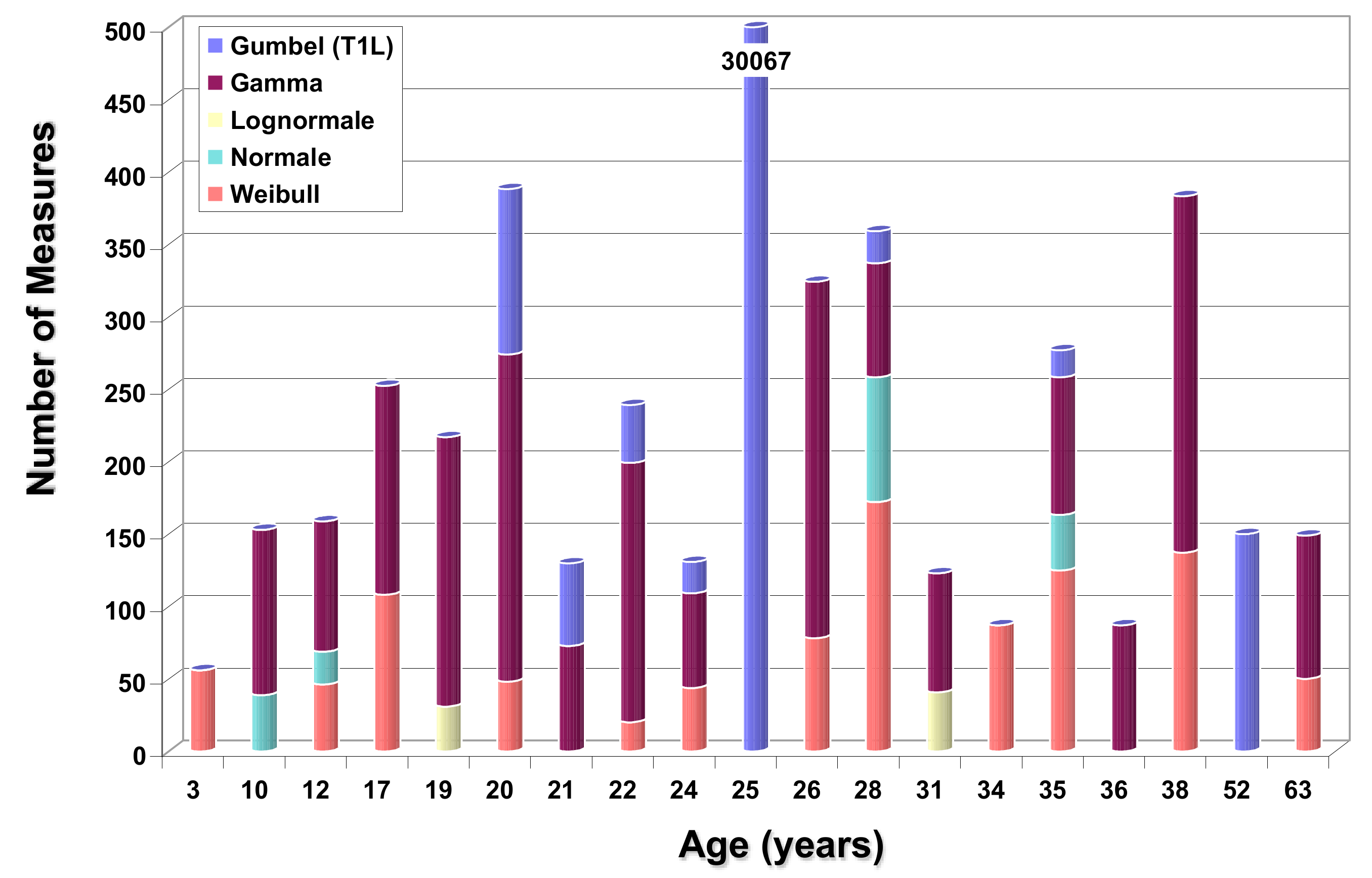
2.4. Crude Statistical Analysis and Selected Method

Keeping in mind these shortcomings, a common idea for exploiting such a database was to perform statistical analysis, one of the common tools for multi-linear correlations being the principal component analysis (PCA) or support vector machine (SVM). The objective was to extract a subset of infrastructures in the harbors where the corrosion in the immersed zone is similar and can be explained by time and other factors given in

Table 1. Bounds for the four corrosion zones in each harbor and normalized bounds.

Harbour			Bounds of Each Corrosion Zone (m)
	ZS		ZT		ZL		ZI		ZM
	Upper Bound MHWS	Lower Bound MHW	Upper Bound MHW	Lower Bound MLW	Upper Bound MLW	Lower Bound MLWS	Upper Bound MLWS	Lower Bound Soil +0.5 m	Upper Bound Soil +0.5 m	Lower Bound Soil −0.5 m
BO	8.85	8.00	8.00	1.86	1.86	1.10	1.10	Depends on each structure	Depends on each structure	Depends on each structure
HA	7.90	7.23	7.239	2.01	2.01	1.20	1.20
PL	0.62	0.59	0.59	0.20	0.20	0.16	0.16
SE	0.62	0.59	0.59	0.20	0.20	0.16	0.16
zN	0.50	0.25	0.25	0.00	0.00	−0.20	−0.20	−0.80	−0.80	−1.20

. Except with the role of time, these analyses were not fruitful. Several explanations can be found:

-

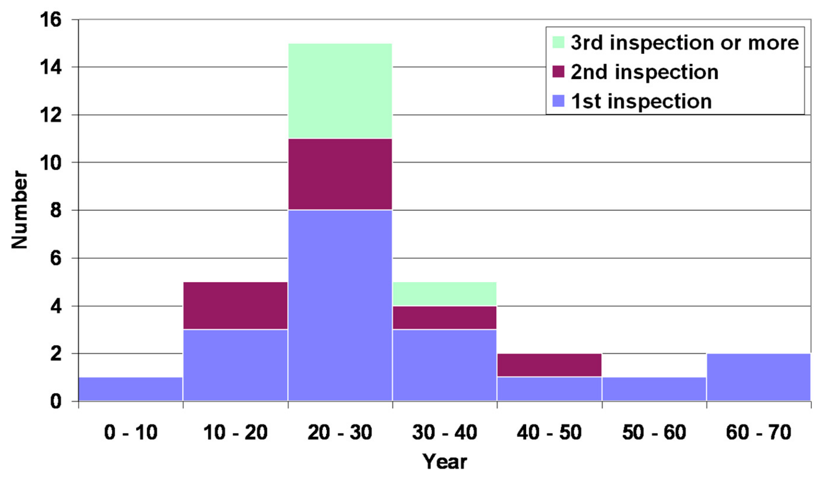
Most of the structures were built between the 50s and the 80s and inspections were carried out 10 to 40 years after when the environmental data was not available until 30 to 50 years after. Knowing the environmental data mainly affects the initial corrosion, this behavior cannot be captured from the database;

-

Environmental parameters were not carried out at the same place but in the same zone and cannot be simply compared since the evolution of these parameters with depth is high ([23] Appendix B 108–111);

-

Kinetics of redox reaction as a function of environmental parameters are non-linear and depend on the relative value and influence of each parameter. Table 1 shows besides that, the order of magnitude of environmental parameters is generally similar and their scatter in each location is high. Moreover, there is a competition of physical-chemical reactions at several scales of time and that cannot be captured due to the sampling of corrosion (one to three over 30 years) and environmental parameters (one to 10 per year);

-

The last point is tricky to analyze when the seasonal and multi-annual variations of these parameters are high. For instance, the Coefficient of Variation (CoV) of suspended materials exceeds 90% in all locations and reaches 200% in one location in the HA harbor and the CoV of temperature and dissolved O2 are respectively higher than 30% and 20% at a single location.

-

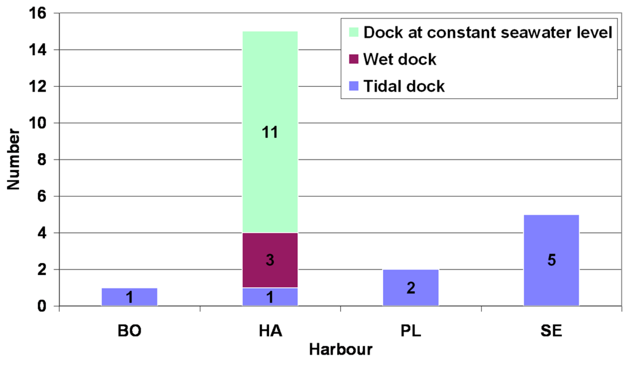
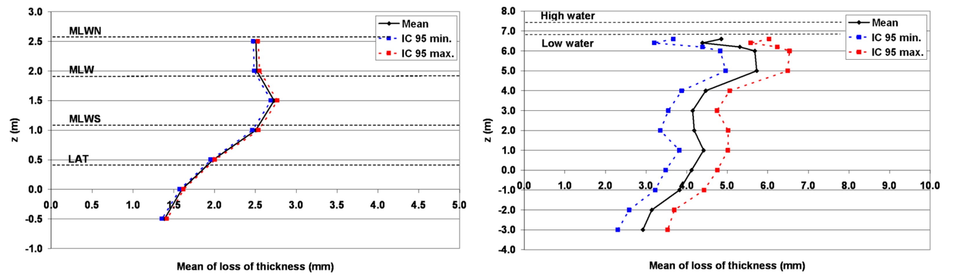
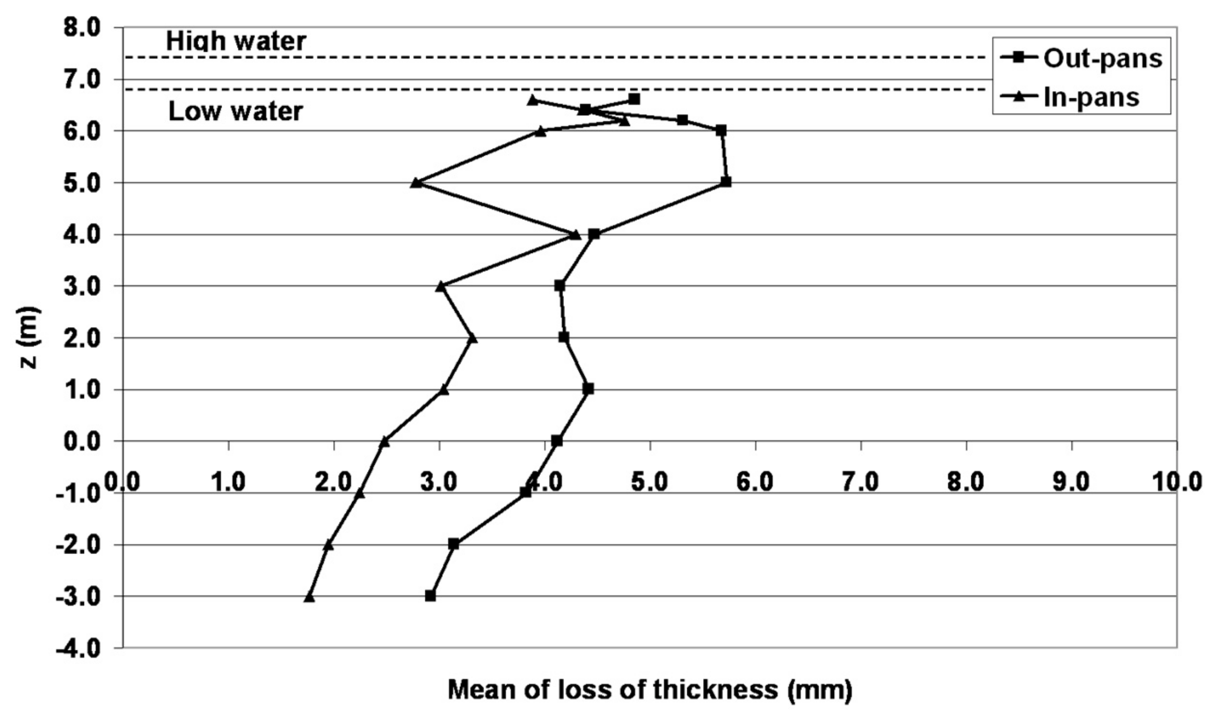
The gradient of the LoT in the immersion area is a well-known phenomenon since 1949 [24,25] and it was recently shown to be the case in harbors with regard to environmental parameters [23]; besides, it depends on the dock type (Figure 4). Knowing that the measurements of corrosion and environmental parameters were not carried out at the same depth, the relationship between parameters and corrosion is highly difficult to capture.

Due to all these limitations and the lack of tangible results, we decided not to investigate further this analysis and to gather all the data of French harbors for probabilistic modeling of corrosion. The next section will hence consider that two factors affect the corrosion in the French database and will be considered as explanatory factors: coordinates in depth and time.

3. Results and Discussion

This section aims at building a statistical-based model of the stochastic (space and time-variants) process of corrosion.

3.1. Modeling Corrosion Stochastic Process with Depth

It has been known for 70 years that the corrosion process is indexed by depth and time. Humble for sheet piles in North Carolina (1949) [24], Edwards for coupons in eight locations in the USA (1963) [25], Songa for harbors in Great Brittany and the Netherlands (1981) [26], and Memet for harbors in France [6], all share the same point of view, as illustrated by Figure 6 (left) [24]: the corrosion profile is varying non-linearly with depth, with ratios up to three between losses of thickness in different zones. The location of these extreme values is of first importance for the estimation of yield bending moment and the structural reliability assessment [19]. However, the exact location of these extreme values is not defined in the literature. Defining these zones and their bounds will be the first focus of this section.

The quantity of measurements between extreme values is limited and the corrosion on these areas has a limited effect on structural reliability [19]. Hence, we model the corrosion random field as a piecewise random field with an area of small height where the extreme corrosion occurs and a uniform level of corrosion between them (see Figure 6 (right)).

At the preliminary stage, an in-depth understanding of the following issues is necessary:

-

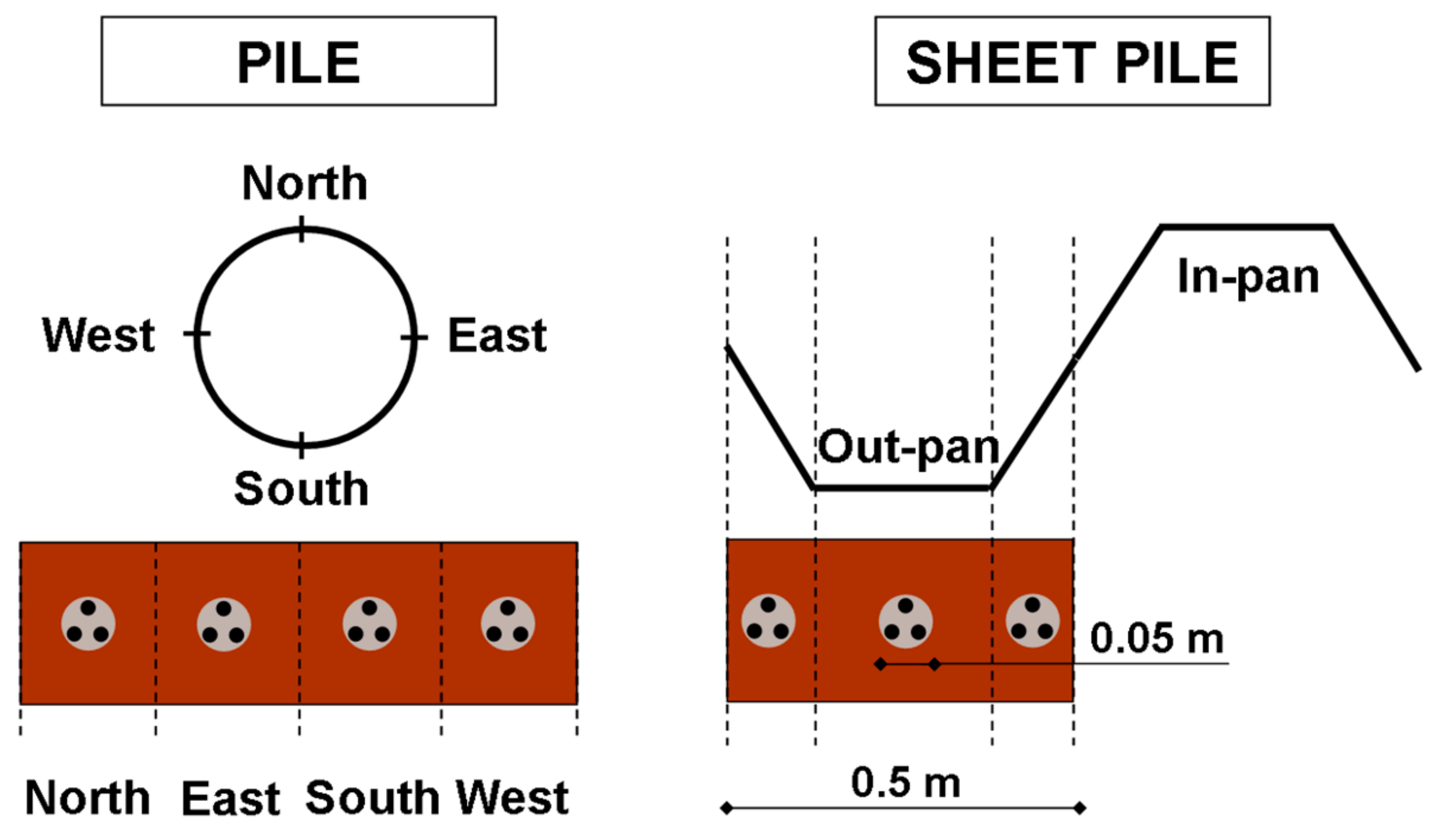
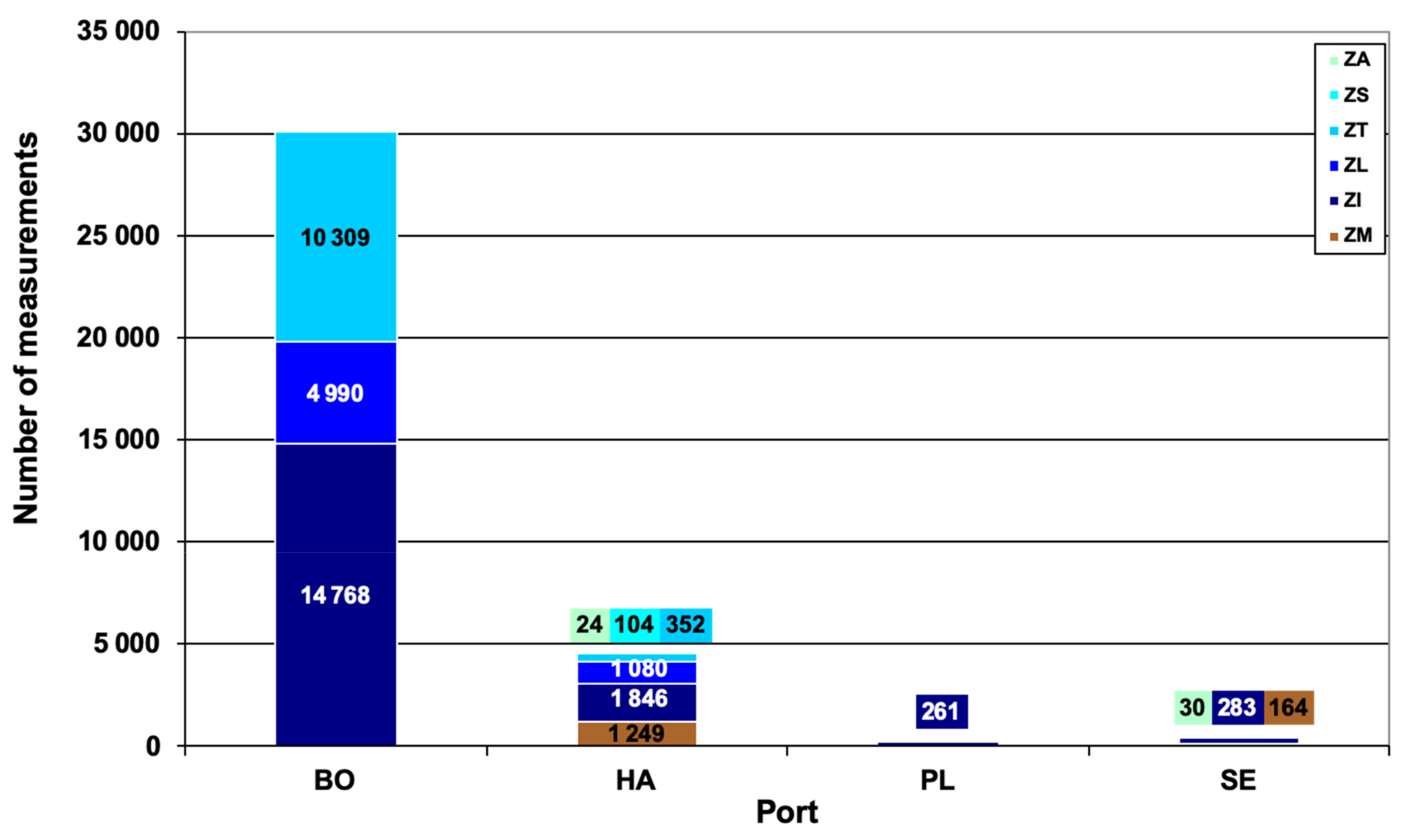
Interpretation of the experimental data (over 35,000 measurements of sheet pile LoT) and the physico-chemical phenomena, which allows spatial corrosion to be treated essentially as a one-dimensional problem according to the depth.

-

Probabilistic modeling in each zone to account for the variability of the phenomena. Having taken the preceding points into consideration, the stochastic time-dependent corrosion model presented in this paper is based on the temporal evolution of parameters for a given probability density function of the random variable “steel LoT” in each exposure zone.

3.2. Definition of Exposure Zones in Relation to Environmental Conditions

The maximum tide level is varying each day and in France twice a day. So, the exposition of points in this key area for corrosion (Figure 6) is varying each day. However, certain tide levels occur more or less frequently and we usually define statistically as the Highest Observed Level, Lowest Observed Level, Mean High Water, Mean Low Water, and Mean Tide Level.

Water sea level is defined statistically as:

-

Mean High Water (MHW);

-

Mean High Water Springs (MHWS);

-

Mean Low Water Springs (MLWS); the arithmetic mean of the low waters occurring at the time of the spring tides observed over a specific 19-year Metonic cycle;

-

Mean Low Water (MLW): the arithmetic mean of the low water heights observed each tidal day;

This directly impacts the duration of exposure to the atmosphere and the kinetics of corrosion. In view to define the areas affected by the tide, we have to define statistically the tide level that bounds two corrosion zones.

First, from the literature review, let us define the five distinct exposure zones to corrosion:

-

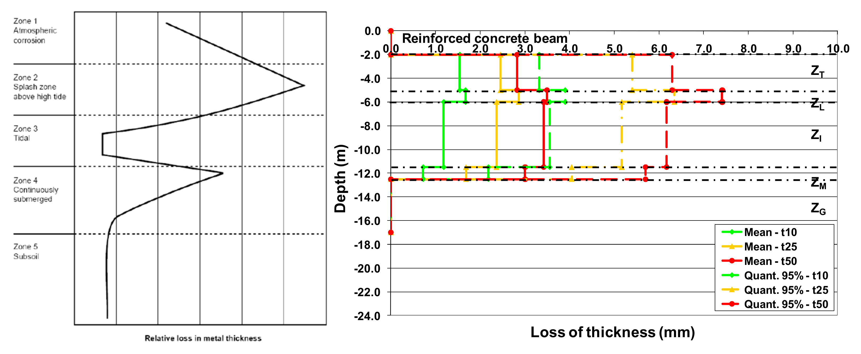
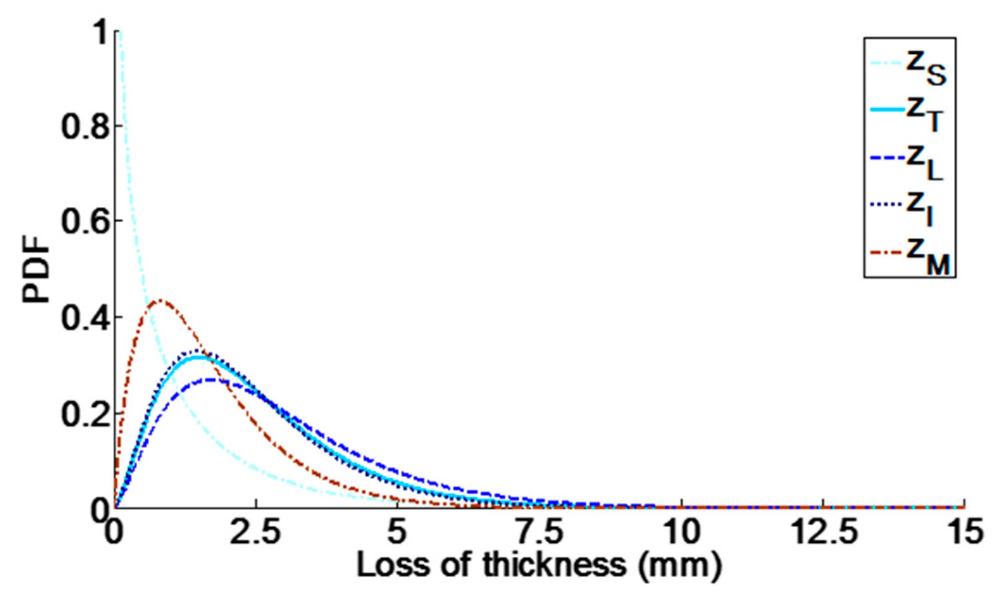
Splash zone (ZS): it is a wetland where a continuous water film is maintained on the surface of metal exposed to the atmosphere. This area is accessible at low tide. The corrosion in this area is particularly active and is manifested locally by densely pickled areas

-

Tidal zone (ZT): this zone is located between the average level of high tides and the average level of low tides and is alternately submerged and emergent. This area is only accessible at low tide at high tide coefficients. The moderate degradation of the metal in this area (corrosion rate in the order of that of the submerged area) is due to partial atmospheric corrosion, together with a cathodic depolarization caused by the highly oxygenated water film deposited by tides in relation to superficial water layers. Therefore, at the interface between the wetland and the submerged area, corrosion cells are produced by different concentrations of oxygen. The metal under the water is anodic and corrosion rates are intense because of short electrical paths

-

Low seawater level zone (ZL): the area of lower waters lies just below the average level of lowest tides. This is the area where corrosion is particularly active because of the differential ventilation battery that is established with the upper structure. The metal top, situated in the tidal zone, highly oxygenated, is a cathode. The metal found just below in the area constantly submerged, is the anode, the seat of a major dissolution of metal.

-

Immersion zone (ZI): this area is located between the area of lowest waters and the mud area. The metal is in permanent contact with seawater and macro-fouling will colonize and grow. This is a difficult area to access for maintenance without using cofferdams or under-water techniques.

-

Mud zone (ZM): this buried area corresponds to the buried parts of a metal structure. The feedback shows that this area usually requires very little maintenance. The top of this level can be inspected in most cases in harbors because sediments can be removed but the conditions of inspection are harsh.

There is usually no atmospheric zone on harbor structures (or a small area—see Figure 5) because the platform is placed in the spray area.

Tide level being stochastic, the exposure zones are defined from statistical analysis of the corrosion profile. Zones of Figure 6 are bound either by a peak in the corrosion profile or a change in the slope. These two criteria were used in our database. Our objective is now to rely on the bounds of the corrosion zone with the environment, particularly the tide level. Let us first highlight that in France, the oscillation amplitude of the semidiurnal tide is associated with a dimension-less coefficient, the tidal coefficient (CMAR) (see [22] for more information and illustrations) has values between 20 and 120. CMAR is computed as follows:

$$CMAR=\frac{\Delta H\left(t\right)}{\Delta H_e}$$

where $\Delta H\left(t\right)$ and $\Delta H_e$ are the difference between high and low tide levels at time t and during mean high water springs and mean low water springs near the equinox date (i.e., 21 March or 21 September).

CMAR assists in finding similar tidal conditions; however, the real water level is affected by other events such as atmospheric pressure and storm surge. In the present study, the distance between measurements (rarely 10 cm and more often 0.5 m) is a limiting factor of accuracy in the definition of the bounds of the exposure zone. These environmental variations are in the same order of magnitude as the distance between measurements and are their effect will not be considered.

The profile of corrosion showed a similar shape to the one in Figure 6 (left). Positions of the bounds of each zone in each harbor are given in Table 1. In view to simplify the following statistical analysis of the corrosion database, we affect each corrosion measurement to a zone from its coordinates. The tide level depends on the geographic location of the harbor along the French coast. Vertical coordinate z was normalized z_N from –1 (interface with soil) to +5 (platform underside) (last line of Table 1). It is shown that whatever the environmental geographic location (Atlantic coast, Channel, Mediterranean coast), the boundaries can be defined by water sea level.

A first overview is given in

Table 2. Average corrosion rates at the four corrosion zones.

Harbour	Duration of Exposure (year)	Average Corrosion Rate (mm/year)
		ZS	ZT	ZL	ZM
BO	25	-	0.10	0.11	0.06
HA	10 to 65	0.03–0.11	0.03–0.08	0.04–0.29	0.01–0.15
PL	34	-	-	0.06	0.03
SE	53 to 63	-	-	0.07–0.11	0.07–0.11

where we give the average corrosion rate in each harbor and each exposure zone. The time period at which it was computed is given in the second column of the table. Note that the boundaries are in the same order of magnitude as those published for reinforced concrete in the marine environment [27]. This comparison is interesting because reinforced concrete is steel with a protective chemical (concrete) layer.

3.3. Pricewise Modeling with Gamma Probability Density Functions

To fully describe the space and time-variant stochastic process, trajectories of data should be analyzed, explained by a physical mechanism, and modeled. It is known that the time-variant modeling changes the reliability assessment [28]. Due to the period between inspections (several years), the time-variant stochastic process cannot be assessed from our database. As a consequence, the auto-correlation with time is not available from the database and no publication suggests such a model until now. Past studies (see introduction) have shown that second-order random variables are able to model the LoT; the following modeling relies thus on the evolution of the average trend and the standard deviation with time. We will compute these statistics by gathering all the data available in each exposure zone defined in the previous section.

The selection of the quantity of interest is the next issue: the modeling could focus on the LoT or the corrosion rate. The last one is useful at the design step when the service life-time is defined by standards (between 30 and 50 years for harbor structures). However, it is well known that the corrosion rate is varying with time due to the reduction of corrosion rate with time. As the objective of the paper is to provide a priori probability density distributions for harbors with time, we chose to model the LoT of standard sheet piles or out-pans of U-shaped sheet piles that have been shown to present similar LoT [23].

Let us first observe some trends. The evolution of the average LoT and 5–95% fractiles, according to z, for two wharves BO1 and HA7d, is presented in Figure 7 from 4605 available data at times of inspection 25 and 63 years respectively for BO1 and HA7d. The trend appears clearly and conforms to the results published in the literature [24].

HA7d has a small seawater variation in the dock (0.6 m); consequently, only two levels are indicated, i.e., high water and low water. Figure 8 illustrates for HA7d the well-known phenomena on the U-shaped piles: out-pans corrode faster than in-pans. (mean values after 63 years).

Concerning the standard deviation, Figure 9 illustrates the same trend as the mean of LoT with depth.

Mean and standard deviations having the same trend with depth, let us focus now on the evolution of the coefficient of variation with depth. Figure 10 illustrates this evolution. This coefficient of variation is quite constant according to z. For wharf BO1, it reaches 0.47. Note that for wharf HA7d, this value is 0.44 for out-pans of sheet piling.

An analysis of corrosion mechanisms shows that the process can be modeled by five independent random variables corresponding to five different exposure zones according to the vertical axis, each one based on a different hazard context. Various second-order pdf are candidates to represent the LoT. In view to select the best candidate, we compute the maximum likelihood estimate (MLE) from the available data in each exposure zone at each inspection time among five pdf: normal, lognormal, Gumbel, Gamma, and Weibull. The corrosion is supposedly uniform for each exposure zone as presented in Figure 6 right but real data shows a slope (Figure 7 right): we keep the maximum value in each exposure zone as the representative value of this zone for each profile. This is a conservative approach and the model should be seen as the distribution of the maximum corrosion in each zone. We plot in Figure 11 the number of measurements whose distribution follows a given pdf according to the MLE. It is shown that both normal and lognormal pdf represent poorly the experimental distribution. That is due to the shape of this distribution. We plot in Figure 12 a typical distribution of LoT in the Low Seawater Zone after 25 years. It shows a typical dissymmetrical shape with non-negligible weak values: thus, both normal and log-normal pdf are rejected. Among the three remaining pdf, it is shown that Gamma pdf is the best candidate for 13 inspection times among a total of 19 (70%). Moreover, Gamma pdf has an interesting property: it tends asymptotically towards an exponential pdf when the shape parameter α reaches 1. This is especially interesting at the early age of the structure when the amount of negligible LoT areas is huge.

3.4. LoT Long Term Space Dependent Model (LoT-TS)

The LoT-TS model is presented in the following. The model relies on the usual assumption that corrosion is seen as a decoupled phenomenon on the $R^2$ plane of a structure; that is, along the length x and the depth z. The trend of corrosion in the x-direction is modeled by a deterministic trend T(x,Z_E,t) which evolves with time t and depends on the exposure zone Z_E (tidal zone, immersion zone, etc.). The mathematical form of this deterministic trend (linear, sinusoidal, etc.) is unique for each asset. It depends mainly on the environmental conditions to which the structure is exposed (marine currents, effluent discharge, etc.). This issue is discussed in [21] and is not detailed in the present paper. As discussed in the previous section, corrosion may be considered as being uniform in the z-direction (Figure 6 right) within a given exposure zone Z_E (tidal zone, immersion zone, etc.). For that reason, only the highest measured LoT in each zone Z_E for a given vertical profile has been selected during the statistical treatment. The corrosion stochastic process of loss of thickness c(Z_E,t,$\theta$), where $\theta$ represents the hazard, is therefore assumed to follow the form in (2), with a dependence on time t and discretized along the depth z by exposure zone Z_E.

c(x,Z_E,t,θ) = T(x,Z_E,t) + c(Z_E,t,θ)

where c(x,Z_E,t,$\theta$) is the space and time-dependent LoT for the exposure zone Z_E (mm), T(x,Z_E,t) is the deterministic trend according to the x-direction and c(Z_E,t,$\theta$) is a random variable representing the LoT with time t for the exposure zone Z_E (mm). We emphasize that the statistical parameters for the random variable c(Z_E,t,$\theta$) may vary throughout the length x, due to the heterogeneity of the environment (concentrated discharges, etc.). After identifying the heterogeneous zones, the random variable c(Z_E,t,$\theta$) can be discretized in the x-direction.

From the previous section, we select the Gamma pdf to model the random variable c(Z_E,t,$\theta$) at a given time. The Gamma pdf is characterized by a shape parameter α and a scale parameter β which are expressed as functions of the two first statistical moments (mean and standard deviation of steel LoT) and which evolves, according to the present model and in the absence of other information on the stochastic structure, in a spatio-temporal way. We chose to drive the stochastic process of corrosion by indexing the pdf parameters in time and space. Mean and standard deviation of data collected in each exposure zone (maximum value on a given profile in this zone) are then computed. A model of the evolution with time is obtained by fitting this empirical evolution using the least-squares method and exponential functions from values of Table 1. Figure 13 presents the fitting of the evolution of the mean and standard deviation of the LoT with time and Figure 14 the Gamma pdf plotted for each zone at time t = 25 years.

In agreement with the literature, the average LoT reaches its maximum value in the area of low seawater level due to the differential aeration which is established between the tidal zone, very oxygenated, and the immersion zone [27]. Moreover, in the mud and immersion zones, this mean trend is increasing with time even after 30 years when stabilization is shown in the tidal zone. That is explained by the well-known effect of anaerobic corrosion [15]. Note that this is, until now, the single long-term model (adapted for corrosion after 30 years) fitted with on-site data available in the literature. We have to underline that the corrosion during the first eight years is not well modeled. Thus, for a short-term reliability analysis where the transition between the aerobic and anaerobic corrosion is needed, another model ([15] for instance) should be preferred.

This parametric modeling of spatio-temporal LoT is very useful in reliability analysis, as well as in engineering for the re-evaluation of corroded structures when fractiles give deterministic values with a given percentage of exceedance. Figure 6 presented the 95% fractiles of the LoT at three exposure times: 10, 25, and 50 years. It shows that the mean of LoT depends on the zone and that the width of the distribution support, illustrated here through the 95% fractile, also varies depending on the area: the dispersion of LoT is larger in area Z_L than in others. This result is emphasized in

Table 3. Main statistics (m: mean; s: standard deviation) of the steel thickness loss obtained from the corrosion model for each zone after 10, 25, and 50 years.

Exposure Zone ZE	t = 10 years				t = 25 years				t = 50 years
	m	s	Cov (%)	95 % Fractie	m	s	Cov (%)	95 % Fractile	m	s	Cov (%)	95 % Fractile
ZT	1.54	0.93	60	3.32	2.46	1.53	62	5.40	2.82	1.81	64	6.30
ZL	1.67	1.15	69	3.90	2.87	1.81	63	6.34	3.50	2.06	59	7.42
ZI	1.18	1.19	101	3.55	2.37	1.46	62	5.17	3.42	1.49	44	6.17
ZM	0.72	0.73	101	2.18	1.68	1.22	72	4.05	3.00	1.44	48	5.70

with the coefficient of variation (CoV) which varies from 44 to 101% depending on depth and time.

4. Conclusions

The spatial variability of steel corrosion in marine environments cannot be objectively modeled in a quantitative way by deterministic models. Thus, a probabilistic model is suggested to predict stochastic fields of corrosion. This model is based on expert judgement and a huge database collected from French owners; readings of the residual thicknesses of steels are measured by ultrasonic non-destructive techniques at several depths, structures, and geographical locations along the French coast during the last three decades. First, a vertical piecewise homogeneous process is justified from previous studies in view to model the variability with depth. Boundaries between these areas are justified both statistically and physically and are shown to be in the same order of magnitude as the corrosion of reinforced concrete structures in the sea environment. Distribution of loss of thickness is shown to follow in a vast majority a gamma pdf. The paper provides the parameters of these pdf in each area and during 50 years. Due to a large number of locations and types of steel and quays, this model is a good candidate to provide prior distribution in maintenance optimization and for structural reliability updating from new inspections.

References

1. Southwell, C.R.; Bultman, J.D.; Hummer, C.W. Estimating Service Life of Steel in Seawater; Schumacher, M., Ed.; Noyes Data Corporation: Park Ridge, NJ, USA, 1979; pp. 374–387. [Google Scholar]
2. Melchers, R.E. Probabilistic Modelling of Marine Corrosion of Steel Specimens. In Proceedings of the Fifth International Offshore and Polar Engineering Conference, International Society of Offshore and Polar Engineers, ISOPE-I-95-311, The Hague, The Netherlands, 11–16 June 1995. [Google Scholar]
3. Melchers, R.E. Probabilistic modelling of immersion marine corrosion. Struct. Saf. Reliab. 1998, 3, 1143–1149. [Google Scholar]
4. Paik, J.K.; Kim, S.K.; Lee, S.K. Probabilistic corrosion rate estimation model for longitudinal strength members of bulk carriers. Ocean Eng. 1998, 25, 837–860. [Google Scholar] [CrossRef]
5. Soares, C.G.; Garbatov, Y. Reliability of maintained, corrosion protected plates subjected to non-linear corrosion and compressive loads. Mar. Struct. 1999, 12, 425–445. [Google Scholar] [CrossRef]
6. Memet, J.B. La Corrosion Marine des Structures Métalliques Portuaires: Étude des Mécanismes D’amorçage et de Croissance des Produits de Corrosion. Ph.D. Thesis, Université de La Rochelle, La Rochelle, France, 2000; p. 164. [Google Scholar]
7. Chernov, B.B.; Ponomarenko, S.A. Physico-Chemical Modelling for the Prediction of Seawater Metal Corrosion. In Proceedings of the 10th International Congress on Marine Corrosion and Fouling, University of Melbourne, Parkville, Australia, February 1999; p. 222. [Google Scholar]
8. Schoefs, F. Sensitivity approach for modelling the environmental loading of marine structures through a matrix response surface. Reliab. Eng. Syst. Saf. 2008, 93, 1004–1017. [Google Scholar] [CrossRef] [Green Version]
9. Paik, J.K.; Thayamballi, A.K. Ultimate strength of ageing ships. J. Eng. Marit. Environ. 2002, 216, 57–77. [Google Scholar] [CrossRef]
10. Paik, J.K.; Thayamballi, A.K. Ultimate Limit State Design of Steel-Plated Structures; John Wiley & Sons: Hoboken, NJ, USA, 2003. [Google Scholar]
11. Qin, S.; Cui, W. Effect of corrosion models on the time-dependent reliability of steel plated elements. Mar. Struct. 2003, 16, 15–34. [Google Scholar] [CrossRef]
12. Van der Toorn, A.; Leatimia, F.; Jongbloed, P.; de Beijer, P.; Louwen, P. Corrosion Aspects in the Port of Rotterdam. In Proceedings of the International Maritime-Port Technology and Development Conference, Singapore, 26–28 September 2008; pp. 1–7. [Google Scholar]
13. Jeffrey, R.; Melchers, R.E. Corrosion Tests of Mild Steel in Temperate Seawater; Research Report; Department of Civil, Surveying and Environmental Engineering, University of Newcastle: Callaghan, Australia, 2001. [Google Scholar]
14. Melchers, R.E. Modelling of marine immersion corrosion for mild and low-alloy steels-part 1: Phenomenological model. Corrosion 2003, 59, 319–334. [Google Scholar] [CrossRef]
15. Melchers, R.E.; Wells, T. Models for the anaerobic phases of marine immersion corrosion. Corros. Sci. 2006, 48, 1791–1811. [Google Scholar] [CrossRef]
16. Melchers, R.E. Modeling and Prediction of Long-Term Corrosion of Steel in Marine Environments. Int. J. Offshore Polar Eng. 2012, 22, 257–263. [Google Scholar]
17. Melchers, R.E. Modelling long term corrosion of steel infrastructure in natural marine environments. Underst. Biocorros. Fundam. Appl. 2014, 66, 213. [Google Scholar]
18. Boéro, J.; Schoefs, F.; Capra, B.; Rouxel, N. Technical management of French harbour structures-Part 1: Description of built assets. PARALIA 2009, 2, 6.1–6.11. [Google Scholar]
19. Boéro, J.; Schoefs, F.; Yañez-Godoy, H.; Capra, B. Time-function reliability of harbour infrastructures from stochastic modelling of corrosion. Eur. J. Environ. Civil Eng. 2012, 16, 1187–1201. [Google Scholar] [CrossRef] [Green Version]
20. Schoefs, F.; Clément, A.; Nouy, A. Assessment of spatially dependent ROC curves for inspection of random fields of defects. Struct. Saf. 2009, 31, 409–419. [Google Scholar] [CrossRef] [Green Version]
21. Boéro, J.; Schoefs, F.; Melchers, R.; Capra, B. Statistical Analysis of Corrosion Process along French Coast. In Proceedings of the 10th Internation Conference on Structural Safety and Reliability, San Francisco, CA, USA, August 31–September 4 2009. [Google Scholar]
22. Schoefs, F.; Le, K.T.; Lanata, F. Response surface meta-models for the assessment of embankment frictional angle stochastic properties from monitoring: Application to harbour structures. Comput. Geotech. 2013, 53, 122–132. [Google Scholar] [CrossRef] [Green Version]
23. Boéro, J. Port Infrastructure Reliability: Innovative Approach of Analysis and Probabilistic Modeling of Inspection Data—Application to the Corrosion of Metallic Structures/Fiabilité des Infrastructures Portuaires: Approche Innovante D’analyse et de Modélisation Probabiliste des Données D’inspection. Application à la Corrosion des Structures Métalliques. Ph.D. Thesis, Université de Nantes, Nantes, France, 26 October 2010. Available online: https://www.researchgate.net/publication/338396402_Fiabilite_des_infrastructures_portuaires_approche_innovante_d%27analyse_et_de_modelisation_probabiliste_des_donnees_d%27inspection_Application_a_la_corrosion_des_structures_metalliques (accessed on 22 January 2020).
24. Humble, H.A. Cathodic Protection of Steel Piling In Sea Water. Corrosion 1949, 5, 292–302. [Google Scholar] [CrossRef]
25. Edwards, W.E. Marine Corrosion: Its Cause and Care. In Proceedings of the Eighth Annual Appalachian Underground Corrosion Short Course; Technical Bulletin; West Virginia University Bulletin: Morgantown, WV, USA, 1963; Volume 69, p. 486. [Google Scholar]
26. Songa, T. SP1—Travaux Réalisés Dans le Domaine de la Corrosion Marine par le Comité Exécutif « Corrosion et Protection de Surface » de la C.C.E . In Proceedings of the Conférence Internationale “L’acier Dans les Structures Marines—Sessions Spéciales et Plénières”, Paris, France, 5–8 October 1981. [Google Scholar]
27. Bourreau, L.; Bouteiller, V.; Gaillet, L.; Schoefs, F.; Thauvin, B.; Schneider, J.; Naar, S. Spatial identification of exposure zones of concrete structures exposed to a marine environment with respect to reinforcement corrosion. Struct. Infrastruct. Eng. 2019, 16, 346–354. [Google Scholar] [CrossRef]
28. Hawchar, L.; El Soueidy, C.P.; Schoefs, F. Polynomial Chaos Expansions for Time-Variant Reliability Problems. Reliab Eng. Syst. Saf. 2017, 167, 406–416. [Google Scholar] [CrossRef]
Figure 1. CETMEF protocol: cardinal points for the pile (left) and location for the sheet pile (right).
Jmse 08 00070 g001
Figure 2. Age distribution of the studied structures at inspection time.
Jmse 08 00070 g002
Figure 3. Distribution of docks types in each harbor.
Jmse 08 00070 g003
Figure 4. Maximum variation of seawater level in each type of dock and harbor.
Jmse 08 00070 g004
Figure 5. Distribution of data (loss of thickness) in the various exposure zones (ZA: Atmospheric zone; ZS: Splash zone; ZT: Tidal zone; ZL: Low seawater level zone; ZI: Immersion zone; ZM: Mud zone).
Jmse 08 00070 g005
Figure 6. Typical profile of corrosion with depth (adapted from [24]) (left). Quantiles of the piecewise uniform corrosion model at two ages (10 and 25 years) (right-adapted from [19]).
Jmse 08 00070 g006
Figure 7. Mean of loss of thickness and 5–95% fractiles (IC) according to z—BO1 (left) and HA7d out-pans (right).
Jmse 08 00070 g007
Figure 8. Mean of loss of thickness on in- and out-pans of sheet piling according to z—HA7d.
Jmse 08 00070 g008
Figure 9. Standard deviation of loss of thickness according to z—BO1.
Jmse 08 00070 g009
Figure 10. Coefficient of variation of loss of thickness according to z—BO1.
Jmse 08 00070 g010
Figure 11. Distribution of the number of measurements that follows a given pdf according to the age of structures.
Jmse 08 00070 g011
Figure 12. Distribution of the LoT after 25 years, in the Low Seawater Zone.
Jmse 08 00070 g012
Figure 13. Evolution of the mean and the standard deviation of loss of thickness with time in each zone (exponential fitting). Legend: ZS = Splash zone; ZT = Tidal zone; ZL = Low seawater level zone; ZI = Immersion zone ; ZM = Mud zone.
Jmse 08 00070 g013
Figure 14. Steel thickness loss distributions obtained from the corrosion model for the different zones over a time period t = 25 years.
Jmse 08 00070 g014