PlanetScope and Landsat 8 Imageries for Bathymetry Mapping

Abstract

Bathymetry has a great importance in coastal projects. Obtaining proper bathymetric information is necessary for navigation, numerical modeling, and coastal zone management studies. Over the past three decades, a number of measuring protocols have been validated for bathymetry mapping, either by means of echosounding or LIght Detection and Ranging (LIDAR). Although these traditional methods hold a high vertical accuracy, they may have limitations in accessibility for some areas. Remote sensing (RS) techniques can be alternatively utilized for bathymetry extraction and update for such cases. The satellite derived bathymetry (SDB) can be analytically or empirically obtained based on various RS datasets with different spatiotemporal resolution. The current study proposes a methodology to spatially enhance the Landsat-derived bathymetry. Two different satellite images, i.e., Landsat and PlantScope with a spatial resolution of 30 and 3 m respectively have been assessed in bathymetry mapping. The Landsat image resolution has been spatially enhanced to match the Planetscope resolution. The panchromatic band of the Landsat image has been downscaled and used for pan-sharpening the multispectral bands. The bathymetry was empirically estimated from the blue and green spectral bands using the linear model by Lyzenga. The SDB model was calibrated using field measurements of water depths observed by a single beam echosounder. The Bathymetry detection methodology has been applied in an area of the Northern coast of Egypt. The SDB from the PlanetScope, Landsat 8 OLI, and Enhanced Landsat 8 OLI were assessed using error analysis. It was found that the Enhanced Landsat has a comparable result with the PlanetScope. The root mean square error is 0.38 and 0.43 m for PlanetScope and Enhanced Landsat, respectively. The current methodology was also tested by the ratio transform model for SDB and the results revealed the same conclusion as the linear model. Thus, the developed algorithm provides SDB using free Landsat images that is of comparable accuracy to the relatively expensive PlanetScope SDB.

1. Introduction

Bathymetry is the measure of water depths to define the seabed terrain. Proper determination of bathymetry is important due to its involvement in multiple applications in the coastal environment. It is used to produce nautical charts to ensure the safety of navigation [1]. Further, it helps in understanding wave climate and hydrodynamics as an input for numerical models [2] and has a significant role in coastal zone management. Also, bathymetric maps contribute in the prediction of climate change consequences.

Conventionally, bathymetric data is collected via various methods such as echosounding and LIght Detection and Ranging (LIDAR) devices. For sounding based techniques, single beam echosounders (SBES) or multi-beam echosounders (MBES) may be alternatively used. As for the LIDAR, either airborne lidar bathymetry (ALB) or LIDAR installed on vessel devices are available tools [3]. Depth samples can be precisely generated in case of utilizing SBES with cost less than MBES. For both sounding types, the constraints are the cost, time & labor consuming and the sensitivity to the sea climate [4]. In addition, some difficulties in accessibility for shallow water, rocky seabed or coral reefs areas. ALB provides quick and accurate bathymetric information especially for quietly clear waters and in nearshore where sounding is least effective. Currently, the satellites around the earth have a wide coverage with frequent revisits. So, satellite derived bathymetry (SDB) attracts a lot of scientists’ concern to explore the satellites ability and limitations of for bathymetry mapping.

The basic rule for the SDB is that different wavelengths of the light spectra are attenuated through water bodies by varies degree. When the light passes through water, it is attenuated by interacting with water column according to Beer’s law. In such a way, several attempts have been implemented for bathymetry estimation using remote sensing (RS) either analytically or empirically. Analytical methods are built up on some of physical parameters that account for atmosphere, water surface state, entire water column properties and bed characteristics [5]. All these considerations are induced in the process of light propagation in water. However, such methods allow bathymetry retrieval with higher accuracy compared to the empirical methods if properly calibrated [6]. Empirical models mathematically study the relationship between the remotely sensed data e.g., digital number/radiance/reflectance and the real water depths. From the fitted relationship, the water depths can be estimated for other points throughout the satellite image.

The attempts to use RS in bathymetric data retrieval was initiated by Lyzenga using aerial multispectral data and radiometric techniques [7]. Analytically, Spitzer and Dirks investigated the flow radiative transfer model to estimate water depths [8]. Other analytical methods have been provided by Benny and Dawson [9] and Philpot [10]. Nevertheless, the most popular empirical approach is the linear band of Lyzenga [11,12] that assumes the observed reflectance is an exponential function of the water depth. Thus, a linear relationship can be produced between water depth and bottom reflectance. After that, Jupp suggested a new empirical algorithm that consists of three consecutive steps, i.e., calculation of depth of penetration (DOP) zones, interpolation of depths within the DOP zone, and the calibration of depths within the DOP zones [13]. Moreover, Stumpf et al. proposed a linear ratio model contrary to the linear band algorithm which succeeded in deriving depths greater than 25 m for clear water state [14]. Many researchers contributed to different empirical methods [15,16,17,18,19,20] using nonlinear or machine learning techniques and different types of sea bottom with wide variety of RS data. Most researchers refer to the widely known approaches as the linear band method by Lyzenga or/and the ratio transform model by Stumpf et al. for comparison and accuracy assessment.

In general, SDB was accomplished via different sources of RS information, varying in spatial and temporal resolutions including Landsat multi spectral scanner, Landsat thematic mapper, and Landsat operational land imager (OLI) [11,12,21,22]. SDB algorithms have been also applied to SEASAT, IKONOS and SPOT6 [14,23,24]. Also, Sentinel-2 constituted another supply for RS data [5].

The main advantage of using Landsat is the free access and the spatiotemporal resolution of the Landsat 8 OLI products, with 30 m spatial resolution and 16 days revisit time. The Landsat 8 OLI sensor collects data from 11 spectral bands with different characteristics as shown in

Table 1. Landsat 8 OLI bands information.

Band Number	Description	Wavelength (µm)	Spatial Resolution (m)
Band 1	Coastal/Aerosol	0.435–0.451	30
Band 2	Blue	0.452–0.512
Band 3	Green	0.533–0.590
Band 4	Red	0.636–0.673
Band 5	Near-infrared	0.851–0.879
Banf 6	Short wavelength infrared	1.566–1.651
Band 7	Short wavelength infrared	2.107–2.294
Band 8	Panchromatic	0.503–0.676	15
Band 9	Cirrus	1.363–1.384	30
Band 10	Thermal-infrared	10.60–11.19	100
Band 11	Thermal-infrared	11.50–12.51

[25]. The assessment criteria of RS data quality (spatiotemporal resolution) depend on the application area. The Landsat 8 OLI multispectral (MS) bands have lower spatial resolution than the simultaneously captured panchromatic (PAN) band with 15 m spatial resolution. Hence, refining the OLI image can be introduced by fusing MS and PAN bands following pan-sharpening approaches [26]. By applying the Pan-sharpening technique, the pixel size of MS image will be the same as the PAN image. Here, additional enhancement has been proposed, i.e., downscaling of PAN band by reducing the band pixel size before image fusion [27,28,29]. Therefore, a downscaling then pan-sharpening technique is suggested to produce a higher spatial resolution image, termed enhanced Landsat image in this manuscript.

On the contrary, high resolution RS data such as WorldView and Quickbird with sub-meter spatial resolution and revisit frequency of one day are commercially available and can be used for SDB. Such sources are more accurate in bathymetry generation but they are rather expensive. Alternatively, Planet Labs provide products from CubeSats that image the earth’s surface with fine spatiotemporal resolution at lower cost. Hence, it is interesting to research how this advancement in RS can be employed in SDB. Poursanidis et al was the first to attempt to enroll Planet data in SDB for fine and accurate bathymetry prediction [30]. Landsat 8 OLI is available freely and its resolution can be improved. Accordingly, a comparison between Landsat OLI, Enhanced Landsat OLI and PlanetScope in SDB has been studied. The SDB algorithms have been applied based on the similar bands (bands wave lengths) for both satellites data.

Planet operates PlanetScope, RapidEye and SkySat release processed data in a variety of formats to serve different uses [31]. Imagery may be captured as a single red-green-blue (RGB) scene or a split-frame with RGB and near-infra-red (NIR) depending on the capability of the satellite. Each PlanetScope satellite is a CubeSat 3U form factor (10 × 10 × 30 cm). The complete PlanetScope constellation of approximately 130 satellites able to image the entire land/water surface of the Earth every day (equating to a daily collection capacity of 340 million km²/day). Planet offers three levels for PlanetScope imagery: A basic scene product (level 1B), an ortho scene product (level 3B) and an ortho tile product (level 3A). The orthorectified scene was designed for a wide variety of applications that require imagery with an accurate geolocation and cartographic projection. These scenes are delivered as visual (RGB) and analytic products as digital number (DN), radiance and surface reflectance (SR). Products are in 3 m spatial resolution and consist of four spectral bands with different characteristics,

Table 2. PlanetScope bands information.

Band Number	Description	Wavelength (µm)	Spatial Resolution (m)
Band 1	Blue	0.455–0.515	3
Band 2	Green	0.500–0.590
Band 3	Red	0.590–0.670
Band 4	Near-infrared	0.780–0.860

.

For Landsat data, the principal spectral bands commonly used for SDB are blue and green bands (B2 and B3) and sometimes other bands are added. Similarly, in PlanetScope blue and green bands (B1 and B2) can be utilized for the same purpose.

The objective of the current research is to compare the nearshore bathymetry obtained using Lyzenga’s linear band algorithm from PlanetScope 3B images and Landsat 8 OLI images (with original resolution and enhanced), using as calibration and validation dataset an acoustic bathymetry of a study site in the Northern coast of Egypt. The goal is to provides SDB using free Landsat images that is of comparable accuracy to the relatively expensive PlanetScope SDB.

Field survey has been conducted for calibration process where the MS bands reflectance’s corresponding to each survey point are computed via image pixels interpolation. The current research proposes a rapid, accurate, and cheap method for deriving bathymetry maps with reasonable spatiotemporal resolutions.

2. Study Area and Datasets

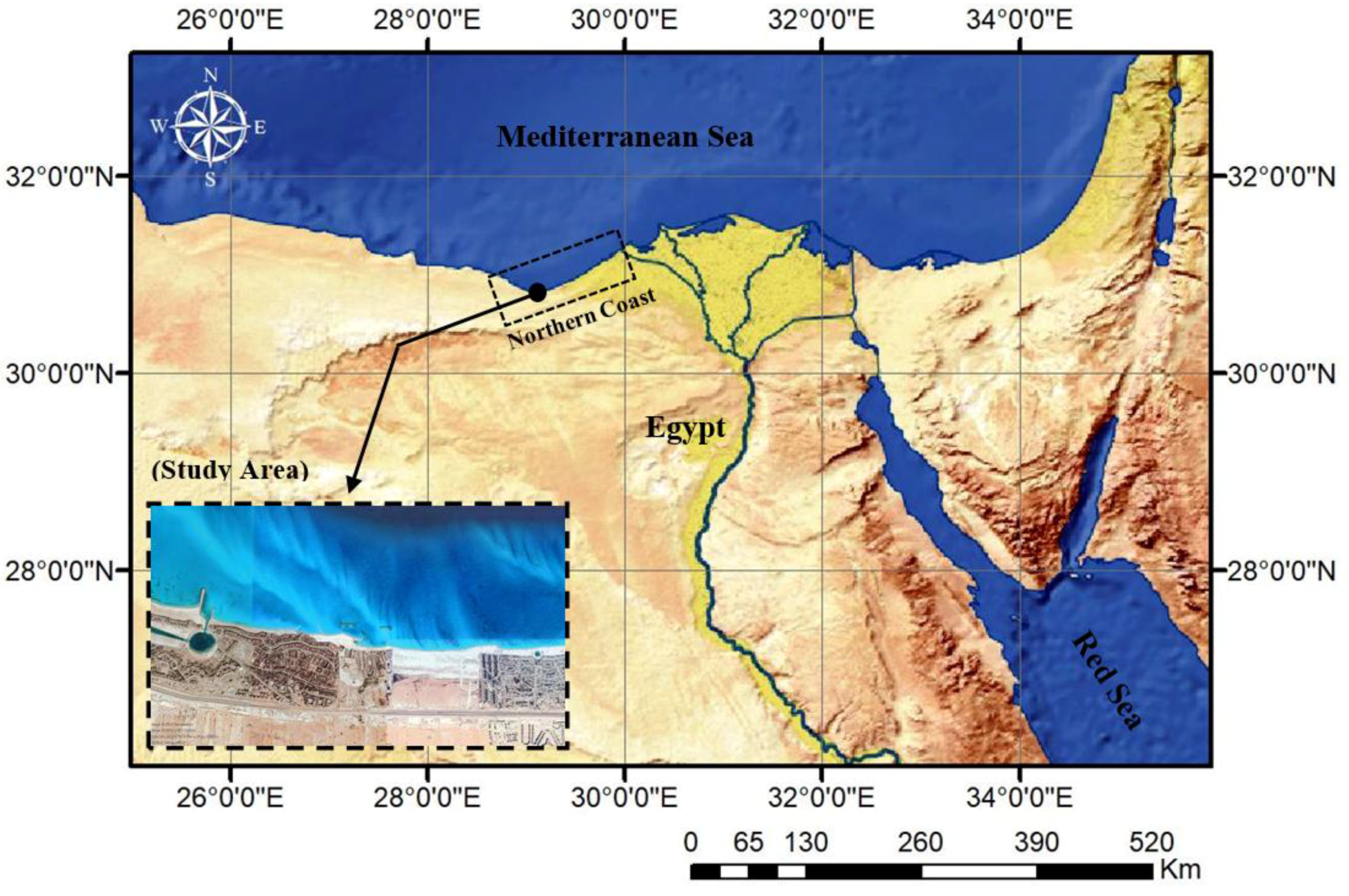
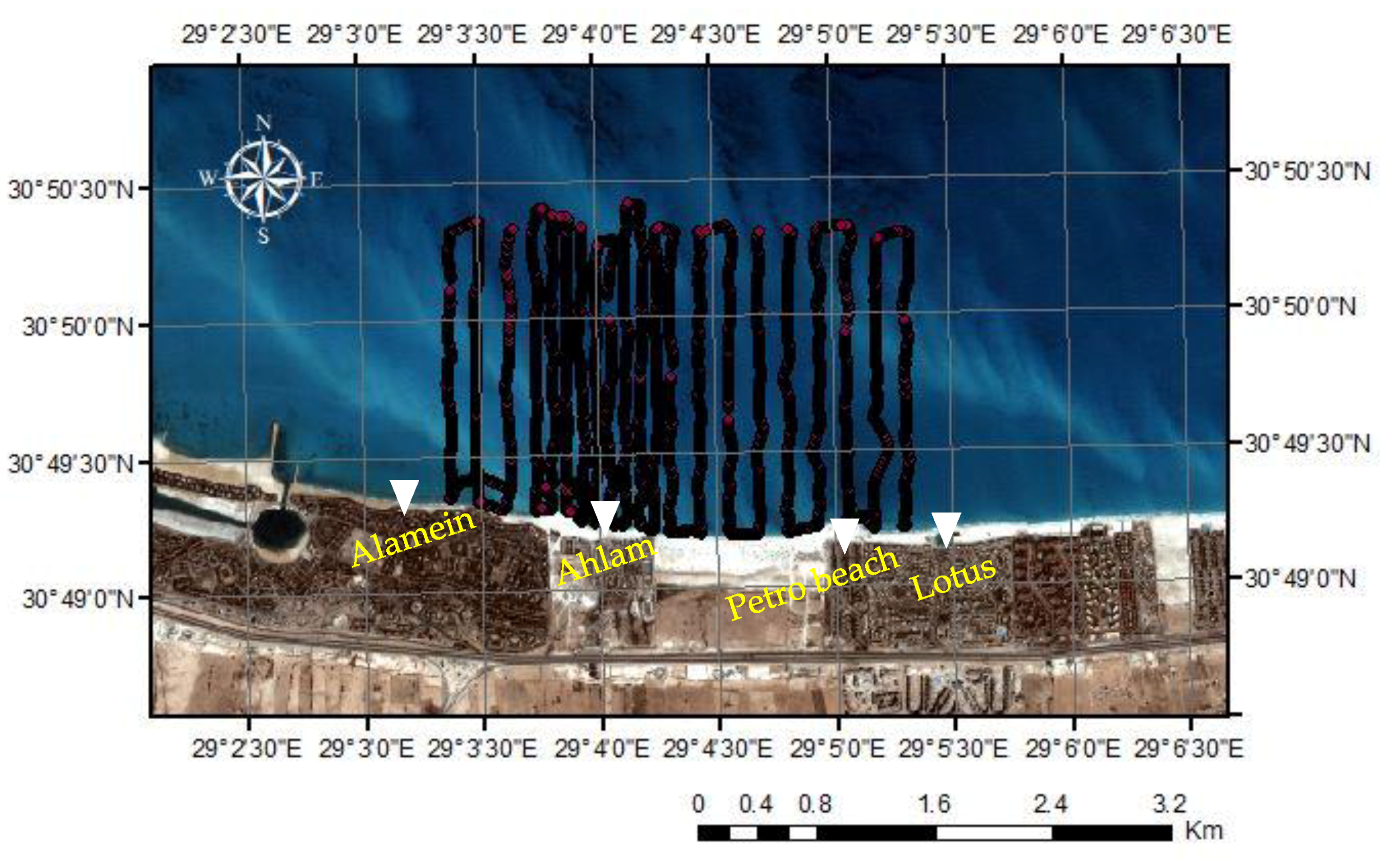
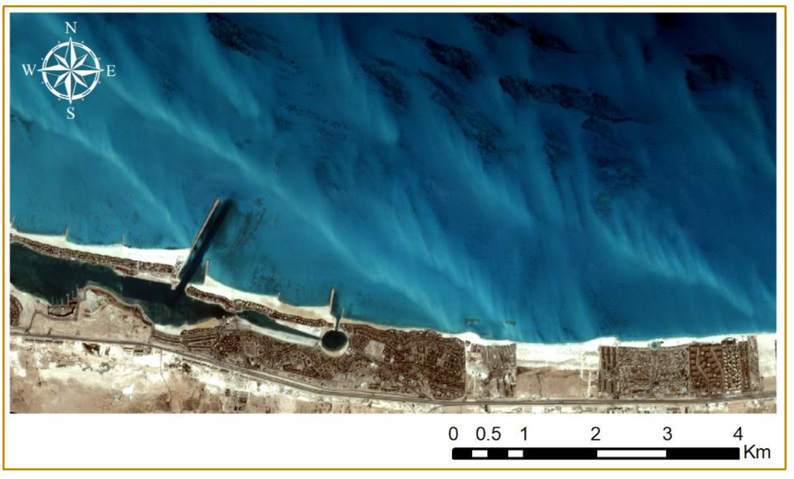
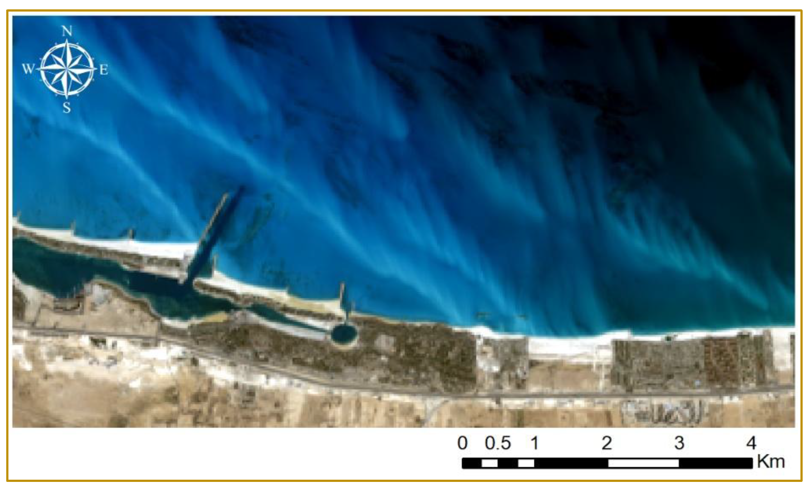
2.1. Study Area

The current study area is bounded by (30°50′25′′, 30°49′11′′) in northing and (29°3′21′′, 29°5′19′′) in easting and located at the North coast of Egypt as presented in Figure 1. It extends about 3.2 km alongshore starting from Marina El Alamein resort in the West to El Lotus resort in the East and 2.2 km in the cross-shore direction as shown in Figure 2. The total coverage of the study area is about 6.77 km². The geomorphology of this area is highly dynamic due to the pro-activity in sediment transport processes. A large amount of sediment is transported from west to the east while several coastal structures exist along the coast that affect the sedimentation behavior. The area includes several features such as sand bars, shelf parts and ridges while the bottom is mostly composed of sand. The water body is almost clear at this region and no coral reefs formation exist. The maximum wave height is close to 5 m and about 40% of approaching waves do not exceed 0.5 m [32]. The highest waves come from the NNW and WNW directions. This area is exposed to a limited portion of waves from N to ENE sector. In this region, the tidal range is small: less than 0.5 m.

2.2. Datasets

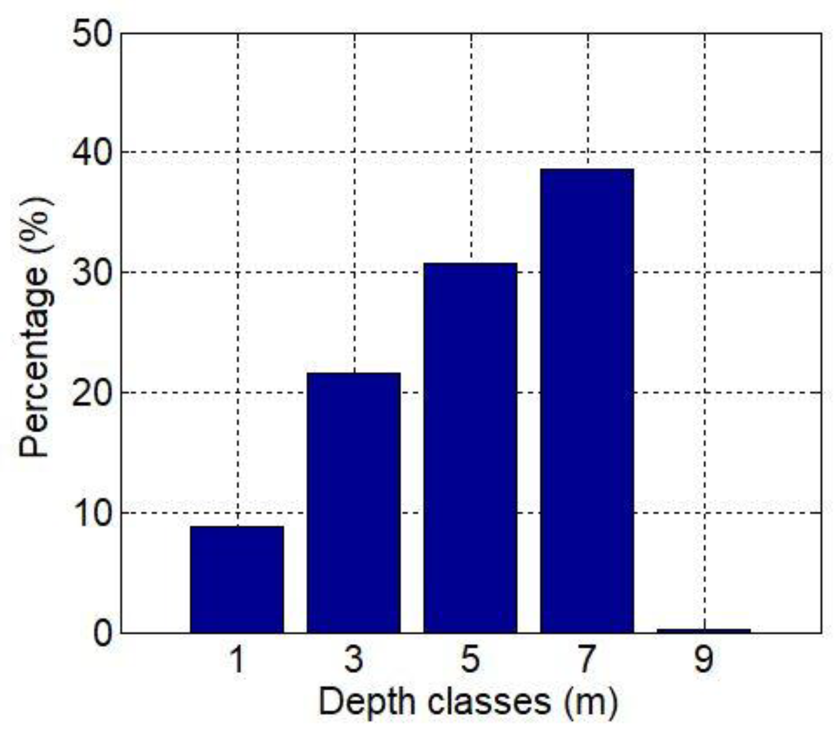
2.2.1. In Situ Data

For bathymetry estimating and testing, measured water depth is required to calibrate the available remotely sensed data. Accordingly, in situ data must be attained either by executing survey or from the available global datasets. So, the accuracy of the calibration data will affect the accuracy of the SDB. Nautical charts and hydrographic charts may be used [33]. Also, light detection and ranging (LiDAR) data can be utilized [22] and many researchers use data from acoustic bathymetry surveys (i.e., acquired with an echosounder) [30]. In the current study, field measurements from extensive bathymetric survey using a single beam echosounder have been used. The devices employed in survey included NavisoundPC100 as a single beam echosounder and Trimble 2000 GPS for horizontal positioning. The recorder of NavisoundPC100 was operated at 200 kHz frequencies with resolution 1 cm of measured depth. The vertical accuracy is 0.01% of total depth and the recording range is from 0 to 30 m. Calibration check of the echosounder was done by means of a bar check. The bar checks were carried out as a supplementary check for velocity of propagation in sea water and also to confirm the transducer draught depth. That was achieved by suspending a round steel plate beneath the transducer face at variable depths (2 to 4 m). The horizontal positioning accuracy of the GPS at 95% confidence level is 5 m + 5% of water depth.

Figure 2 shows the echosounder paths and the surveyed points distribution within the studied domain. The echosounder observations were collected during the day of 14th September 2019 and gathered depths of 7659 points. The water depths varied from 0.38 m to 8.37 m. Figure 3 gives an informative representation of the measured depths frequencies.

2.2.2. Remote Sensing Data of PlanetScope

The PlanetScope image used in this research belongs to the level 3B (orthorectified scene) products. The 3-m pixel image data is available as raw DNs, at sensor Top of Atmosphere (TOA) reflectance’s or atmospherically corrected SR. The used image for SDB is the already processed SR product. Regarding the processing made by Planetscope Lab, the image is radiometrically corrected using sensor telemetry and a sensor model. It is geometrically corrected using ground control points (GCPs) and fine digital elevation models with 30 m to 90 m resolution and projected to a cartographic map projection, i.e., UTM WGS84. Atmospheric effects are accounted for using 6SV2.1 radiative transfer code. AOD, water vapor and ozone inputs are retrieved from MODIS near real time data. The used image shown in Figure 4 was acquired at 29th September 2019 with central scene time of 08:23:05.68 UTC and origin of X = 684,123, y = 3,419,832 UTM WGS84. The cloud cover, sun azimuth and sun elevation were 0.01%, 142.9° and 50.5° respectively. A visual inspection of the RGB images does not show a sun glint effect. In addition, no sun glint was identified by inspecting the NIR values as no significant variation exists. Before using the image in the bathymetry algorithm, it was cropped to the region of interest (ROI) and SR was converted to scaled SR.

2.2.3. Remote Sensing Data of Landsat

The Landsat satellite imagery is commonly used for SDB. These imaging platforms were established and operated by the U.S. geological survey. Seven satellites; from Landsat 1 to 5 in addition to Landsat 7 and 8; were launched for remotely gathering earth surface data from space and the current mission is Landsat 8. Landsat 8 satellite is orbited at 705 kilometers and carries OLI and thermal infrared sensor (TIRS). OLI and TIRS collect image data for nine shortwave bands (from band 1 to band 9) and two longwave thermal bands (band 10 and band 11). The ultra-blue band 1 is useful for coastal and aerosol studies while band 9 is useful for cirrus cloud detection. Thermal bands 10 and 11 are useful in providing more accurate surface temperatures and are collected at 100 m resolution. The approximate scene size is 170 km by 183 km. A satellite image at level 1 from Landsat 8 OLI data sets was used in this study; shown in Figure 5. The image was acquired at date of 5th October 2019 with scene center time of 08:36:35 UTC. It was chosen based on the full coverage of proposed site, minimum cloud cover and the temporal proximity to both of bathymetric survey date and PlanetScope image acquisition date. The cloud cover, sun azimuth, and sun elevation are 0.01%, 149.08°, and 50.52°, respectively. The image is less affected by sun glint and no correction is required; the same tests as applied on Planetscope were performed. The image was cropped to fit the study area. Further, in parallel, the Landsat image was then enhanced, and its spatial resolution was refined via downscaling of the panchromatic band and pan-sharpening of MS bands.

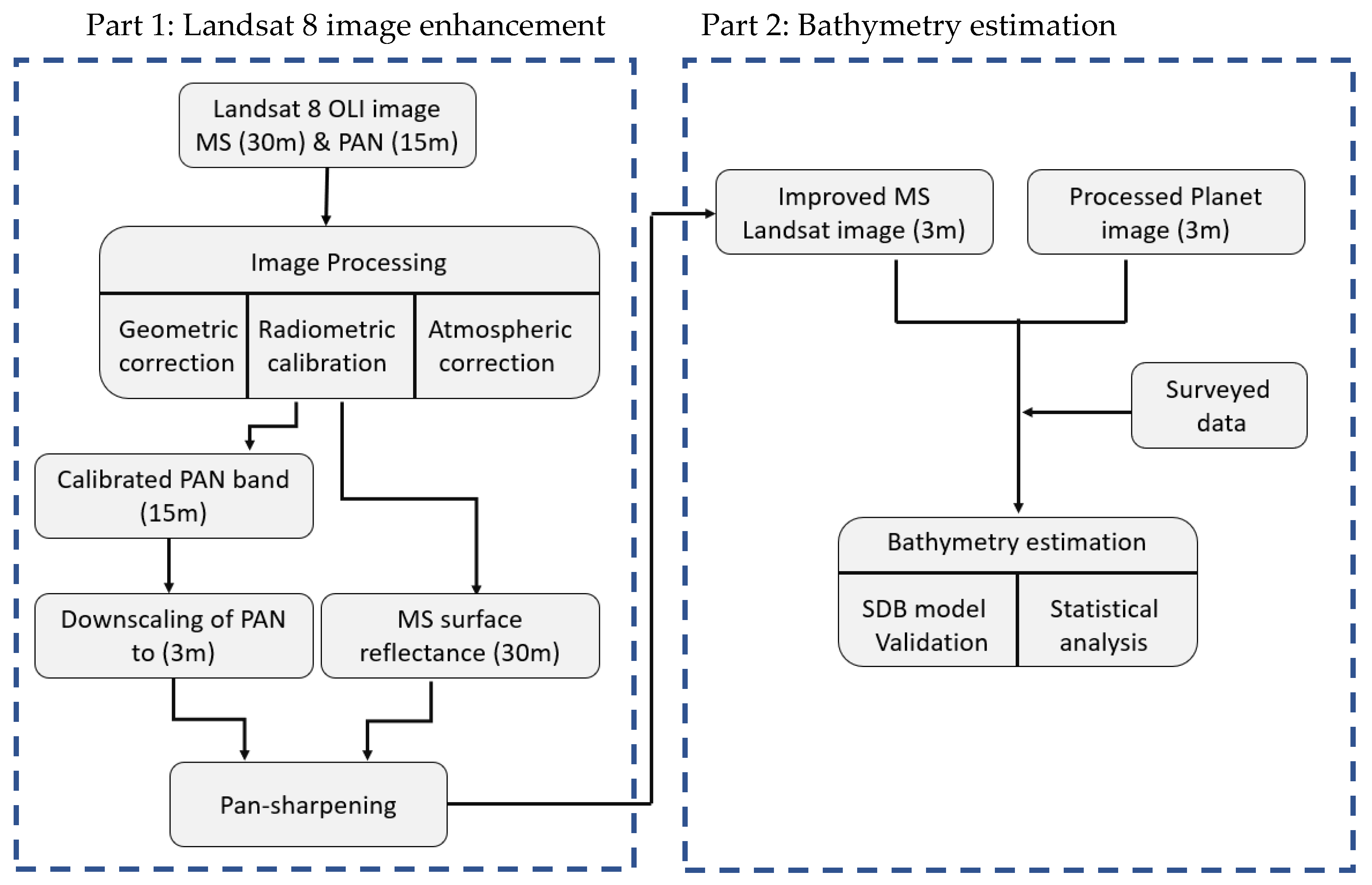
3. Methodology

Figure 6 summarizes the implemented research methodology. The methodology is mainly composed of two major parts, Landsat 8 OLI image enhancement and bathymetry extraction. The aim of the enhancement procedure is testing the improvement of SDB accuracy caused by an increased image spatial resolution. Prior to this stage, the Landsat image has been geometrically and atmospherically corrected. As the Landsat 8 OLI is available with a panchromatic band with higher resolution of 15 m, it is useful to merge this band with the multispectral bands to refine the MS resolution. Various approaches differing in their assumptions and theoretical basis, known as pan-sharpening, have been designed for this image fusion. Some of these pan-sharpening methods are included in the widely known RS software such as ENVI or ERDAS IMAGINE. A procedure was adapted to lower the PAN pixel size (downscaling) before pan-sharpening. The bathymetric data was estimated based on the produced downscaled & pan-sharpened image of Landsat 8 OLI and the readily processed PlanetScope 3B in parallel. Bathymetry was attained empirically by the linear band algorithm by Lyzenga based on the green and blue bands reflectance. In bathymetry prediction, the bathymetry derivation model was validated with the measured in-situ data and the results were statistically evaluated using error analysis.

3.1. Landsat Image Enhancement

3.1.1. Image Processing

With different configurations of sensors characteristics, atmospheric conditions and image acquisition aspects, satellite imagery products needed to be normalized. Image processing is preliminarily implemented on RS scenes before utilizing and analyzing their data. Further, it is critically necessary because the extracted features from the image are sensitive to the process scheme. Processing is mainly proposed to eliminate the image distortion caused by any unwanted path-radiance and other atmospheric effects. Processing is commonly performed through three major steps, i.e., geometric correction, radiometric calibration, and atmospheric correction.

Geometrically, both PlanetScope and Landsat images were geo-referenced using GCPs with WGS84 UTM zone 35 projection to assure elimination of any rotation and shift within the images. Although the imageries are geo-referenced and provided in UTM projection, it is better to re-correct the images using the GCPs to improve the precision of geo-locations. So, four GCPs within the study area were used for this correction; two points at Marina El Alamein and other two points at El Lotus. Radiometric calibration is basically executed to convert the image DNs to TOA reflectance. PlanetScope 3B orthorectified scene has been already processed. Landsat images were radiometrically calibrated using the ENVI Radiometric Calibration tool. Atmospheric correction is necessary to reduce some atmospheric impacts negatively affect the light reflectance. This correction was only applied to the Landsat image as PlanetScope 3B images had been already corrected.

The fast line of sight atmospheric analysis of spectral hypercubes (FLAASH) model of ENVI is commonly used to subtract the atmospheric errors in the Landsat scene [34]. Hence, it was used to atmospherically correct the Landsat image. The FLAASH algorithm uses as radiative transfer model the moderate resolution atmospheric transmission (MODTRAN) that corrects wavelengths in the visible through NIR and shortwave infrared regions, up to 3 µm. The input image for FLAASH is a radiometrically calibrated radiance image in band interleaved by line format. The module further takes into consideration the date of acquisition, time as well as the sensor altitude for further correction of the image. The tool uses a dark pixel reflectance ratio method to retrieve the aerosol amount and estimate the average scene visibility [35]. One of the standard MODTRAN models is chosen according to the expected surface temperature of the RS scene.

Finally, PlanetScope 3B and Landsat OLI reflectance’s were scaled to values from 0 to 1 using the band math suit in ENVI software. These scaled reflectance values were the input data used for deriving bathymetry empirically.

3.1.2. Downscaling

Downscaling is powerfully used in RS to refine the spatial resolution of coarse images. Atkinson defined the downscaling terms, its importance in RS and critically reviewed most of the methods and operators [36]. Commonly, interpolation methods or geostatistical tools as bilinear, spline, kriging and others are alternatively utilized for satellite image downscaling [36]. Kriging is one of the advanced geostatistical modules estimate surfaces from a scattered set of z-values. It requires an interactive investigation of some phenomenon demonstrated by the inputs to tune the best model parameters used for generating the output surface [37]. There are two Kriging methods: ordinary and universal. Ordinary Kriging is the most popular among the kriging family used for interpolation. In the current research, downscaling was configured based on ordinary Kriging. It was applied to reduce the observed PAN band pixel size from 15 m to 3 m to match the PlanetScope image resolution. The Kriging and the related parameters optimization were accomplished by ArcGIS software.

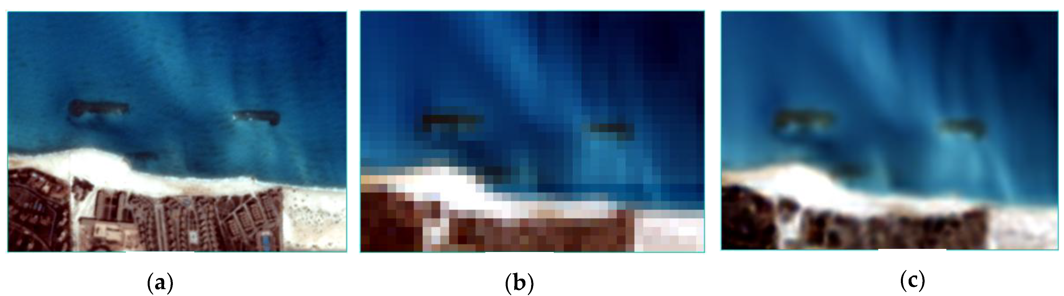
3.1.3. Pan-sharpening

Pan-sharpening is a resolution merge between a high spatial resolution image and a coarse spatial resolution MS image preserving the spectral features of the original MS image [38,39]. Several studies contributed to sharpening developing and concentrated on extracting multiple land surface features from different imageries [40,41]. Two categories of pan-sharpening techniques exist, i.e., component substitution (CS) based and multi resolution analysis (MRA) based techniques [42]. Among the CS based algorithms is intensity hue saturation (IHS) [43,44], principal component analysis (PCA) [38,45,46], Gram Schmidt (GS) [41,47], Brovey transform (Brovey) [48], partial replacement adaptive component substitution (PRACS) [49]. While the MRA based algorithms include high pass filtering (HPF) [42], smoothing-filter-based intensity modulation (SFIM) [50], additive injection model (Indusion) [51], additive à trous wavelet transform (ATWT) [52,53], and additive wavelet luminance proportional (AWLP) [54] among others. MRA-based techniques for pan-sharpening has a superiority to the CS-based type in fusing Landsat 8 OLI images especially, Indusion, ATWT and AWLP; they are the most accurate and achieve realistic visualizations [55]. Accordingly, ATWT was selected to conduct the MS image sharpening mission. Finally, a fine spatial resolution image in the form of downscaled PAN band (3 m) was fused into the 30 m MS Landsat data, transforming it to a 3-m resolution MS image.

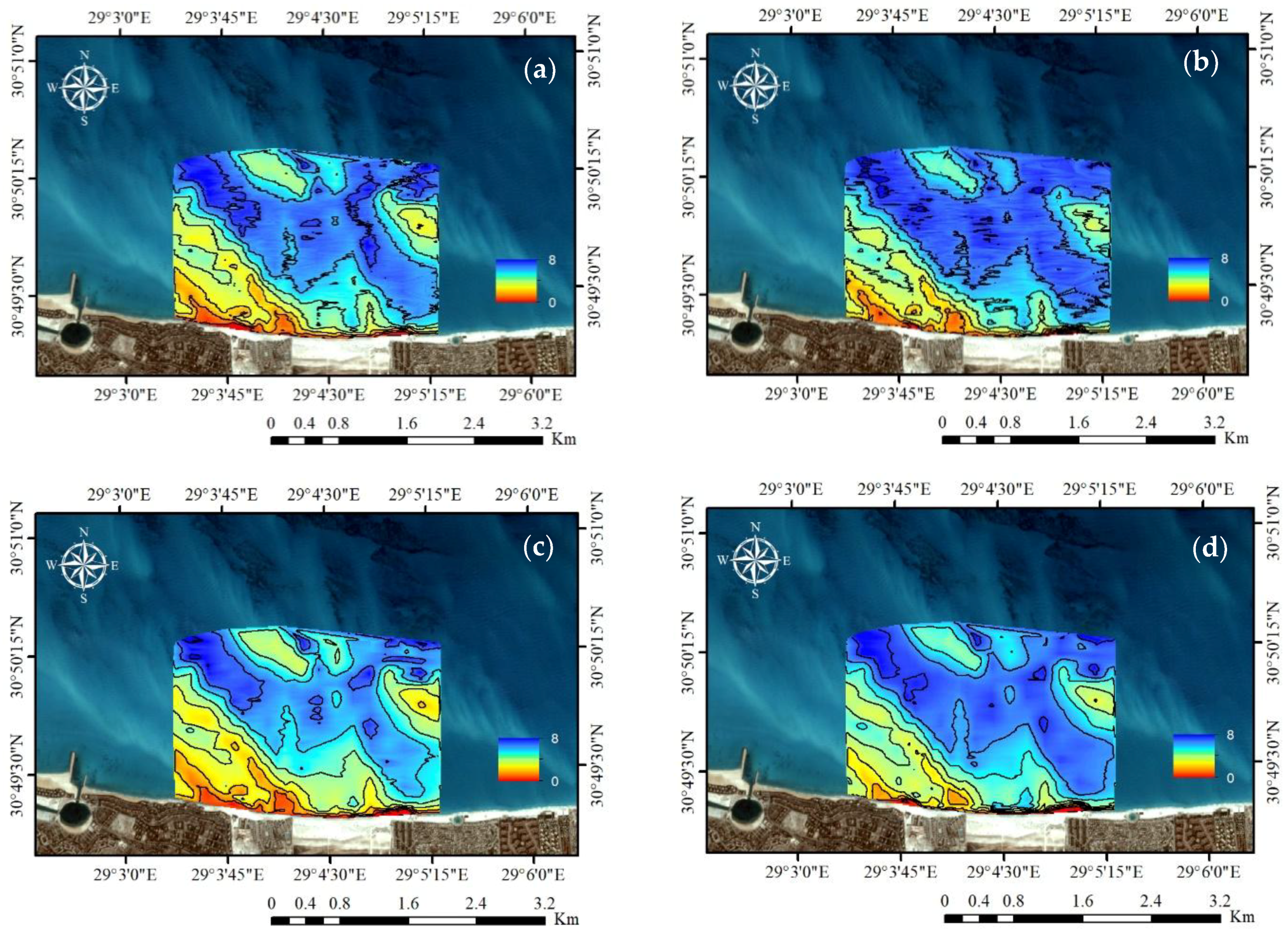
3.2. Bathymetry Estimation

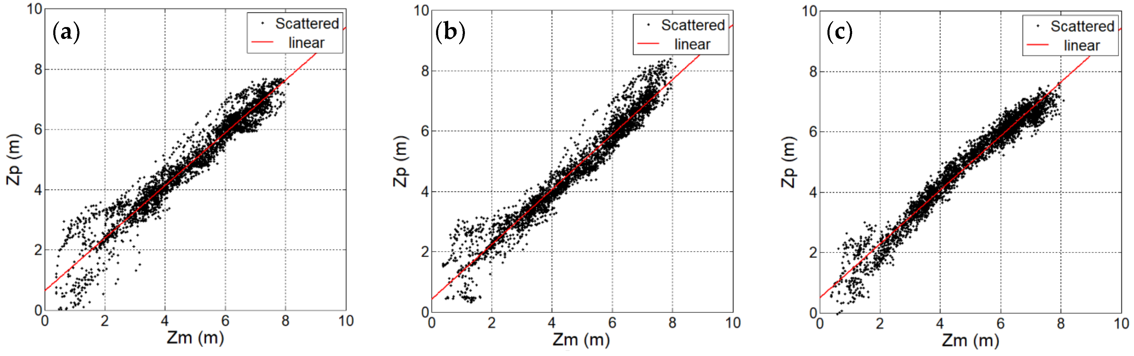
3.2.1. SDB Model Validation

The depth calculation was carried out empirically. The empirical approaches include constructing a mathematical relationship between the field measurements and RS data. In this way, 60% of the measured water depths randomly distributed within the study area has been utilized to build the SDB model while, the rest of data has been used to evaluate the model validity via error analysis. Since the required data either field measurements or RS data were readily collected and prepared, a decision is needed to decide which SDB model will be used. In the current study, the linear band algorithm by Lyzenga [11,12] was applied as an efficient method for shallow water bathymetry mapping as field surveyed depths is less than 10 m. Additionally, it was validated for use in literature for both Landsat 8 OLI and PlanetScope 3B data [20,30]. In general, the bands with shorter wavelengths like blue and green are preferred for the SDB because of their strong penetration proficiency. So, the blue and green bands were utilized in the linear band model of bathymetry derivation. Lyzenga model assumes the water surface reflectance is an exponential function of the water depth. So, a linear relationship can be estimated between water depth and surface reflectance. It is formulated as follows:

$$Z=a_{°}+{\displaystyle \sum }_i^n{a}_i{X}_i$$

(1)

where,

• Z is the water depth
• $X_i=Ln\left(R_i-Rd{p}_i\right)$
• $R_i$ is the observed reflectance in each band.
• $Rd{p}_i$ is the reflectance of dark water pixels.
• $a_{°}$ and $a_i$ are regression coefficients from the relation between the measured depths and the bands reflectance based on least square error.
• n is the number of spectral bands contributes in the linear regression.

If imagery has already been atmospherically corrected then, $X_i$ = Ln ($R_i$) [56]. This model is not restricted to only two bands, i.e., three bands such as coastal aerosol, blue, and green can be utilized in bathymetry estimation [22].

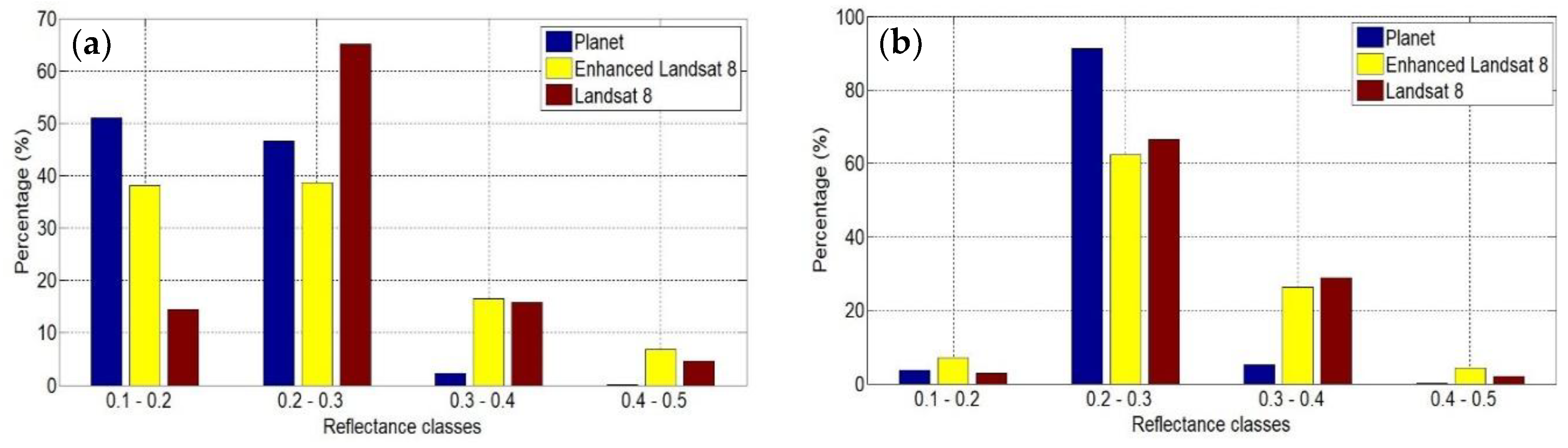
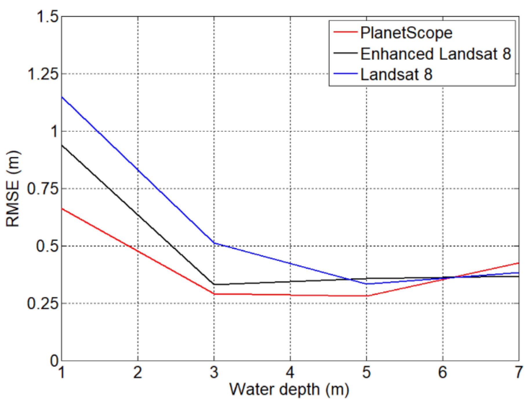
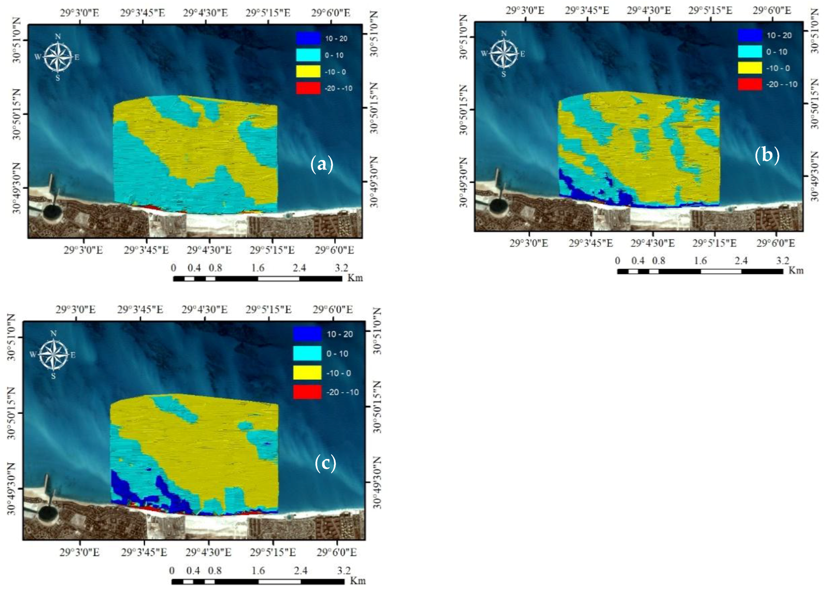
3.2.2. Statistical Analysis

Based on 60% of field measurements, three bathymetries were generated for the three different scenes; PlanetScope 3B, Landsat 8 OLI and Enhanced Landsat 8 OLI. In order to evaluate the outputs of these images and compare them with the measured data, a statistical analysis has been applied to the other 40% of field measurements via variable parameters including the bias, the root mean square error, the mean absolute error, and the coefficient of determination. The parameters are defined as follows:

$$\mathrm{Bias}=\mathrm{Mean}\left({\mathrm{Z}}_{\mathrm{p}}\right)-\mathrm{Mean}\left({\mathrm{Z}}_{\mathrm{m}}\right)$$

(2)

$$\mathrm{RMSE}=\sqrt{{\displaystyle \sum }_1^{\mathrm{N}}{\left({\mathrm{Z}}_{\mathrm{p}}-{\mathrm{Z}}_{\mathrm{m}}\right)}^2/\mathrm{N}}$$

(3)

$$\mathrm{MAE}=\frac{1}{\mathrm{N}}{\displaystyle \sum }_{\mathrm{I}}^{\mathrm{N}}\left|{\mathrm{Z}}_{\mathrm{p}}-{\mathrm{Z}}_{\mathrm{m}}\right|$$

(4)

$${\mathrm{R}}^2=\left[{\displaystyle \sum }_1^{\mathrm{N}}{\left({\mathrm{Z}}_{\mathrm{m}}-{\mathrm{Z}}_{\mathrm{p}}\right)}^2/{\displaystyle \sum }_1^{\mathrm{N}}{\left({\mathrm{Z}}_{\mathrm{m}}-\mathrm{Mean}\left({\mathrm{Z}}_{\mathrm{m}}\right)\right)}^2\right]$$

(5)

where,

• ${\mathrm{Z}}_{\mathrm{p}}$ is the predicted depth from satellite imagery.
• ${\mathrm{Z}}_{\mathrm{m}}$ is the measured water depth.
• N is the number of field measurements.

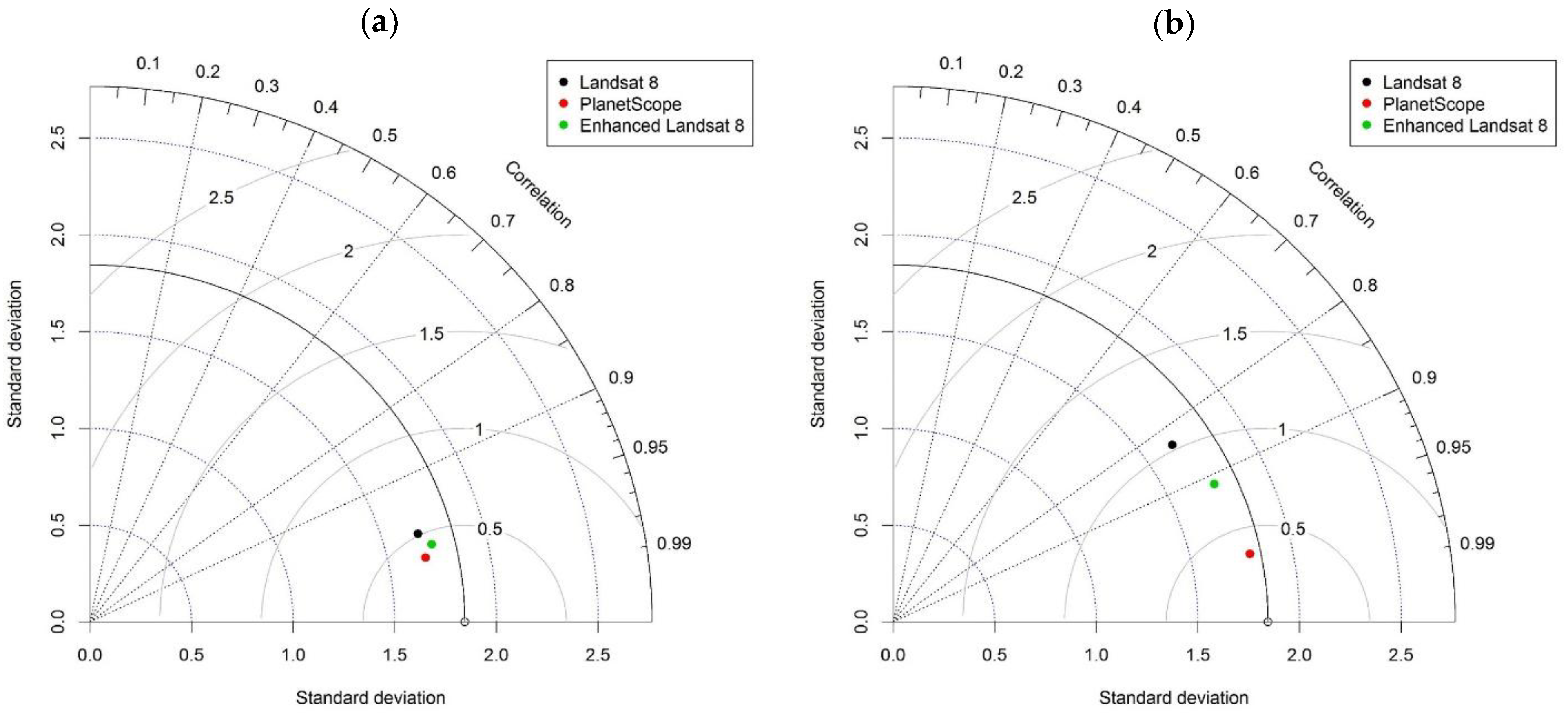
4. Results and Discussion

Three images were developed using the three sources described above to estimate the water depths. Figure 7 demonstrates samples of PlanetScope 3B, Landsat 8 OLI and the enhanced Landsat 8 OLI images. Visually, the enhanced Landsat 8 OLI roughly approaches the quality of the high-resolution image of PlanetSope 3B. The raw Landsat 8 OLI image is visually less fine than the others.

Since the input for the bathymetry estimation model were the blue and green bands reflectance, these reflectance values were obtained from three images for each point of the measured water depths. The blue and green bands are bands 2 and 3 for Landsat 8 OLI image while they are band 1 and band 2 for PlanetScope image. Figure 8 provides the scaled reflectance values distribution for the blue and green bands related to each imagery type. It is observed that, for both bands, the different imagery sources depict a similar pattern.

The Lyzenga model coefficients; a_o, a₁ and a₂ were obtained through a multi-linear regression between the measured water depths and reflectances of blue and green bands, as illustrated in

Table 3. Linear band algorithm coefficients for the different imageries.

Image	ao	a1	a2
PlanetScope	−3.24	14.72	−18.48
Enhanced Landsat 8 OLI	−0.37	3.78	−6.07
Landsat 8 OLI	−2.84	2.72	−5.98

. Three equations have been developed for the three different images; PlanetScope 3B, Landsat 8 OLI and Enhanced Landsat 8 OLI. Firstly, in order to evaluate the model performance for each image data, the correlation between measured and predicted water depths was computed in form of R². As observed in

Table 4. Statistical analysis summary for the estimated bathymetries from the different satellite imageries.

Image	R2	RMSE (m)	MAE (m)	Bias (m)
PlanetScope	0.96	0.38	0.30	−0.024
Enhanced Landsat 8 OLI	0.95	0.43	0.32	−0.013
Landsat 8 OLI	0.93	0.51	0.37	0.026

and Figure 9, all images prove a good linear trend, while the best relationship is developed from PlanetScope data; R² = 0.96. This result appears better than that achieved by [30] for nearly similar water depth range (0–10) m and using Planetscope imagery; R² = 0.88. On the contrary, Landsat 8 OLI without enhancement had the lowest value of R²; 0.93 and then the enhanced Landsat 8 OLI; R² = 0.95. The real water depths versus the model predictions were more concentrated around the line in case of PlanetScope. Conversely, dispersions varying from moderate to high for Enhanced Landsat 8 OLI and Landsat 8 OLI respectively. This scattering especially appears and increases for the lower water depths. In all cases, the linear band model overestimated the water depths less than 2 m with variable degrees for each imagery type. Higher predicted depths mean lower recorded reflectances by the satellite sensors. Since the model was calibrated, water depth can be predicted for any location within the study area, Figure 10.

On other hand, root mean square error (RMSE) and mean absolute error (MAE) were calculated for each image as an indicator for the produced error, Table 4. For PlanetScope, the predicted bathymetry was the best among the images achieving the lowest error; RMSE = 0.38 m and MAE = 0.30 m. This obtained RMSE is better than the resulted error by [30] for the SDB from Planetscope; RMSE = 0.88 m for water depths (0–10) m. The raw Landsat 8 OLI product produced the highest errors; RMSE = 0.51 m and MAE = 0.37 m and enhancing image had a positive effect reducing the errors to RMSE = 0.43 m and MAE = 0.32 m. Accordingly, upon RMSE and MAE, PlanetScope RS data was the best in retrieving bathymetry and the enhanced Landsat 8 OLI bathymetry is so close to it. Regarding the bias, the shift of means between measured and predicted depths was found as negligible for all retrieved bathymetries, as shown in Table 4.

Additionally, water depths were gathered into clusters to partially evaluate the error distribution within each zone. That is to clarify the error related to each region and the parts holding low or high error concentration. RMSE was represented for each mid-point of depth class according to the three different imagery types, Figure 11. In general, at the higher water depths (>5) m, the error was decreasing for all images while especially the PlanetScope was better performing. The depths from (3–5) m had a larger error values than first zone (>5) m. For the remaining depths (<3) m, the error was higher due to the model overestimations as illustrated earlier. It is also observed that PlanetScope and enhanced Landsat 8 OLI had the same changes in error with depth. A unique behavior was observed for Landsat 8 OLI data, in which the error was much larger than for the other images.

Alternatively, the percentage of error in water depths were estimated through the region of interest (ROI). That was to express the deviation in the estimated depths with respect to the measured values. The percentage of error in water depth was computed by subtracting the measured from the estimated and then the dividing by the measured depth. The variability in water depth estimates was around ±20% and concentrated in the shallower depths such as the western side of the ROI, in Figure 12. For PlanetScope, the portions corresponding to percentage of error ranges (>−10), (−10–0), (0–10) and (>10) % were 0.25%, 50.11%, 48.36%, and 1.28% respectively. Around 98.47% of the percentage of error was within ±10% and that ensures the efficiency of PLanetScope in bathymetry retrieval. Similarly, the percentages of the same ranges were obtained from enhanced Landsat 8 OLI were 11.70%, 32.90%, 54.48%, and 0.92% respectively. So, 87.38% of the percentage of error is within ±10% and that is so closer to PlanetScope results. Also, for Landsat 8 OLI these percentages were changed to 12.12%, 24.44%, 60.20%, and 3.24% respectively. Thus, 84.64% of the percentage of error was within ±10% and that is the lowest achievable performance compared to other imageries.

In order to validate the methodology of the current research, the ratio transform method for SDB by Stumpf et al. [14] was investigated against the linear method of Lyzenga. Ratio transform model was calibrated and tested with the same approach as the linear model. The analysis of testing results for both linear model and Stumpf et al model was summarized in the Taylor diagram, depicted in Figure 13. Taylor diagram shows the correlations, RMSEs and standard deviations of predictions for the three different images based on both SDB models. For the three images, ratio transform models achieved lower correlations and higher RMSEs than linear models. The correlations of ratio transform models were from 0.84 to 0.98, while for the linear models were from to 0.96 to 0.98. The produced RMSEs were from 0.37 m to 1.03 m for ratio transform model while from 0.38 to 0.51 for the linear model. However, the linear model performed better than the ratio transform model, as the model of Stumpf et al. proves the previous conclusion that PlanetScope is better than Landsat 8 OLI in estimating bathymetry and the Landsat 8 OLI image enhancement has a positive impact on the obtained SDB.

5. Conclusions

The current research presents a methodology for estimating coastal bathymetry from two different RS datasets, one is the commercial product of PlanetScope and the other is the freely available Landsat 8 OLI data. PlanetScope is an orthorectified scene level 3B with 3 m spatial resolution while Landsat 8 OLI data contains a 30 m spatial resolution for multispectral bands and a 15 m panchromatic band. In the procedure, the Landsat 8 OLI image was downscaled and pan-sharpened in order to match the same pixel size of PlanetScope image. The panchromatic band was fused to the multispectral bands using kriging and ATWT as interpolation and pan-sharpening techniques respectively. The methodology was applied to a region located at the North coast of Egypt which is characterized by the clear water, sandy bottom and absence of coral reefs.

The objective was to assess the accuracy of the satellite derived bathymetry from the three images; PlanetScope 3B, Landsat 8 OLI and enhanced Landsat 8 OLI. Firstly, Landsat 8 OLI image was radiometrically calibrated, geometrically and atmospherically corrected. PlanetScope image was just georeferenced because it was attained in a processed format. Three bathymetries were produced based on linear band model. The linear model was calibrated via 60% of field measurements of water depths acquired by a single beam echosounder till depth nearly 8.37 m. The remaining 40% of the measured water depths randomly distributed within the study area were used to test and evaluate the model via error analysis.

The error analysis revealed that, for the three images, a good correlation between the measured and predicted water depth was achieved. For Planetscope, enhanced Landsat 8 OLI and Landsat 8 OLI images, the R² were found to be 0.96, 0.95, and 0.93 while the RMSE were 0.38, 0.43, and 0.51, respectively. PlanetScope 3B product is a promising estimator for coastal bathymetry and the enhanced Landsat 8 OLI can predict bathymetry with similar accuracy with a much lower cost. This conclusion was assured by using the ratio transform model for the SDB by the current methodology.

The developed approach generates bathymetry of adequate quality to be used in a variety of fields such as coastal zone monitoring and management.

References

- Gao, J. Bathymetric mapping by means of remote sensing: Methods, accuracy and limitations. Prog. Phys. Geogr. Earth Environ. 2009, 33, 103–116. [Google Scholar] [CrossRef]
- Roelvink, J.A.; Reniers, A.J.H.M. A guide to coastal morphology modeling. Adv. Coast. Ocean Eng. 2011, 12, 3–21. [Google Scholar]
- Saylam, K.; Hupp, J.R.; Averett, A.R.; Gutelius, W.F.; Gelhar, B.W. Airborne lidar bathymetry: Assessing quality assurance and quality control methods with Leica Chiroptera examples. Int. J. Remote Sens. 2018, 39, 2518–2542. [Google Scholar] [CrossRef]
- Guenther, G.C. Airborne lidar bathymetry. Digit. Elev. Model Technol. Appl. DEM Users Man. 2007, 2, 253–320. [Google Scholar]
- Caballero, I.; Stumpf, R.P. Retrieval of nearshore bathymetry from Sentinel-2A and 2B satellites in South Florida coastal waters. Estuar. Coast. Shelf Sci. 2019, 226, 106277. [Google Scholar] [CrossRef]
- Hamylton, S.; Hedley, J.; Beaman, R. Derivation of high-resolution bathymetry from multispectral satellite imagery: A comparison of empirical and optimisation methods through geographical error analysis. Remote Sens. 2015, 7, 16257–16273. [Google Scholar] [CrossRef]
- Lyzenga, D.R. Passive remote sensing techniques for mapping water depth and bottom features. Appl. Opt. 1978, 17, 379–383. [Google Scholar] [CrossRef] [PubMed]
- Spitzer, D.; Dirks, R.J. Shallow water bathymetry and bottom classification by means of the Landsat and SPOT optical scanners. In Proceedings of the 1986 International Symposium/Innsbruck, Innsbruck, Austria, 25 November 1986. [Google Scholar]
- Benny, A.H.; Dawson, G.J. Satellite imagery as an aid to bathymetric charting in the Red Sea. Cartogr. J. 1983, 20, 5–16. [Google Scholar] [CrossRef]
- Philpot, W.D. Bathymetric mapping with passive multispectral imagery. Appl. Opt. 1989, 28, 1569–1578. [Google Scholar] [CrossRef] [PubMed]
- Lyzenga, D.R. Remote sensing of bottom reflectance and water attenuation parameters in shallow water using aircraft and Landsat data. Int. J. Remote Sens. 1981, 2, 71–82. [Google Scholar] [CrossRef]
- Lyzenga, D.R. Shallow-water bathymetry using combined lidar and passive multispectral scanner data. Int. J. Remote Sens. 1985, 6, 115–125. [Google Scholar] [CrossRef]
- JUPP, D.L. Background and extensions to depth of penetration (DOP) mapping in shallow coastal waters. In Proceedings of the Symposium on Remote Sensing of the Coastal Zone International Symposium, Gold Coast, Queensland, Australia, 7–9 September 1988. [Google Scholar]
- Stumpf, R.P.; Holderied, K.; Sinclair, M. Determination of water depth with high-resolution satellite imagery over variable bottom types. Limnol. Oceanogr. 2003, 48, 547–556. [Google Scholar] [CrossRef]
- Gholamalifard, M.; Kutser, T.; Esmaili-Sari, A.; Abkar, A.; Naimi, B. Remotely sensed empirical modeling of bathymetry in the Southeastern Caspian Sea. Remote Sens. 2013, 5, 2746–2762. [Google Scholar] [CrossRef]
- Liu, Q.; Trinder, J.C.; Turner, I.L. Automatic super-resolution shoreline change monitoring using Landsat archival data: A case study at Narrabeen–Collaroy Beach, Australia. J. Appl. Remote Sens. 2017, 11. [Google Scholar] [CrossRef]
- Mondal, I.; Bandyopadhyay, J.; Dhara, S. Detecting shoreline changing trends using principle component analysis in Sagar Island, West Bengal, India. Spat. Inf. Res. 2017, 25, 67–73. [Google Scholar] [CrossRef]
- Misra, A.; Vojinovic, Z.; Ramakrishnan, B.; Luijendijk, A.; Ranasinghe, R. Shallow water bathymetry mapping using Support Vector Machine (SVM) technique and multispectral imagery. Int. J. Remote Sens. 2018, 39, 4431–4450. [Google Scholar] [CrossRef]
- Shen, X.; Jiang, L.; Li, Q. Retrieval of Near-Shore Bathymetry From Multispectral Satellite Images Using Generalized Additive Models. IEEE Geosci. Remote Sens. Lett. 2018, 16, 922–926. [Google Scholar] [CrossRef]
- Gabr, B.; Ahmed, M. Assessment of Genetic Algorthim in Developing Bathymetry Using Multispectral Landsat Images. In Proceedings of the International Conference on Asian and Pacific Coasts, Hanoi, Vietnam, 25–28 September 2019. [Google Scholar]
- Clark, R.K.; Fay, T.H.; Walker, C.L. Bathymetry using thematic mapper imagery. In Proceedings of the 1988 Technical Symposium on Optics, Electro-Optics, and Sensors, Orlando, FL, USA, 12 August 1988. [Google Scholar]
- Pacheco, A.; Horta, J.; Loureiro, C.; Ferreira, Ó. Retrieval of nearshore bathymetry from Landsat 8 images: A tool for coastal monitoring in shallow waters. Remote Sens. Environ. 2015, 159, 102–116. [Google Scholar] [CrossRef]
- Dixon, T.H.; Naraghi, M.; McNutt, M.K.; Smith, S.M. Bathymetric prediction from Seasat altimeter data. J. Geophys. Res. 1983, 88, 1563–1571. [Google Scholar] [CrossRef]
- Manessa, M.D.; Haidar, M.; Hartuti, M.; Kresnawati, D.K. Determination of the best methodology for bathymetry mapping using Spot 6 Imagery: A study of 12 empirical Algorithms. Int. J. Remote Sens. Earth Sci. 2018, 14, 127–136. [Google Scholar] [CrossRef]
- Zanter, K. Landsat 8 data users handbook. 2016. Available online: https://landsat.usgs.gov/landsat-8-l8-data-users-handbook (accessed on 28 June 2019).
- Medina, A.; Marcello, J.; Rodriguez, D.; Eugenio, F.; Martin, J. Quality evaluation of pansharpening techniques on different land cover types. In Proceedings of the 2012 IEEE International Geoscience and Remote Sensing Symposium, Munich, Germany, 22–27 July 2012. [Google Scholar]
- Atkinson, P.M.; Pardo-Iguzquiza, E.; Chica-Olmo, M. Downscaling cokriging for super-resolution mapping of continua in remotely sensed images. IEEE Trans. Geosci. Remote Sens. 2008, 46, 573–580. [Google Scholar] [CrossRef]
- Wang, Q.; Shi, W.; Atkinson, P.M.; Pardo-Igúzquiza, E. A new geostatistical solution to remote sensing image downscaling. IEEE Trans. Geosci. Remote Sens. 2015, 54, 386–396. [Google Scholar] [CrossRef]
- Wang, X.; Liu, Y.; Ling, F.; Xu, S. Fine spatial resolution coastline extraction from Landsat-8 OLI imagery by integrating downscaling and pansharpening approaches. Remote Sens. Lett. 2018, 9, 314–323. [Google Scholar] [CrossRef]
- Poursanidis, D.; Traganos, D.; Chrysoulakis, N.; Reinartz, P. Cubesats Allow High Spatiotemporal Estimates of Satellite-Derived Bathymetry. Remote Sens. 2019, 11, 1299. [Google Scholar] [CrossRef]
- Planet. Planet Imagery Product Specification. 2018. Available online: https://assets.planet.com/docs/Combined-Imagery-Product-Spec-Dec-2018.pdf (accessed on 12 June 2019).
- Frihy, O.; Deabes, E. Erosion chain reaction at El Alamein Resorts on the western Mediterranean coast of Egypt. Coast. Eng. 2012, 69, 12–18. [Google Scholar] [CrossRef]
- Jagalingam, P.; Akshaya, B.J.; Hegde, A.V. Bathymetry mapping using Landsat 8 satellite imagery. Procedia Eng. 2015, 116, 560–566. [Google Scholar] [CrossRef]
- Wang, X.; Liu, Y.; Ling, F.; Liu, Y.; Fang, F. Spatio-Temporal change detection of Ningbo coastline using Landsat time-series images during 1976–2015. ISPRS Int. J. Geo-Inf. 2017, 6, 68. [Google Scholar] [CrossRef]
- Kaufman, Y.J.; Wald, A.E.; Remer, L.A.; Gao, B.C.; Li, R.R.; Flynn, L. The MODIS 2.1-/spl mu/m channel-correlation with visible reflectance for use in remote sensing of aerosol. IEEE Trans. Geosci. Remote Sens. 1997, 35, 1286–1298. [Google Scholar] [CrossRef]
- Atkinson, P.M. Downscaling in remote sensing. Int. J. Appl. Earth Obs. Geoinf. 2013, 22, 106–114. [Google Scholar] [CrossRef]
- Oliver, M.A.; Webster, R. Kriging: A method of interpolation for geographical information systems. Int. J. Geogr. Inf. Syst. 1990, 4, 313–332. [Google Scholar] [CrossRef]
- Amro, I.; Mateos, J.; Vega, M.; Molina, R.; Katsaggelos, A.K. A survey of classical methods and new trends in pansharpening of multispectral images. EURASIP J. Adv. Signal Process. 2011, 2011, 1–22. [Google Scholar] [CrossRef]
- Xu, Q.; Zhang, Y.; Li, B. Recent advances in pansharpening and key problems in applications. Int. J. Image Data Fusion 2014, 5, 175–195. [Google Scholar] [CrossRef]
- Sidek, O.; Quadri, S.A. A review of data fusion models and systems. Int. J. Image Data Fusion 2012, 3, 3–21. [Google Scholar] [CrossRef]
- Ehlers, M.; Klonus, S.; Johan Åstrand, P.; Rosso, P. Multi-sensor image fusion for pansharpening in remote sensing. Int. J. Image Data Fusion 2010, 1, 25–45. [Google Scholar] [CrossRef]
- Aiazzi, B.; Baronti, S.; Lotti, F.; Selva, M. A comparison between global and context-adaptive pansharpening of multispectral images. IEEE Geosci. Remote Sens. Lett. 2009, 6, 302–306. [Google Scholar] [CrossRef]
- Carper, W.; Lillesand, T.; Kiefer, R. The use of intensity-hue-saturation transformations for merging SPOT panchromatic and multispectral image data. Photogramm. Eng. Remote Sens. 1990, 56, 459–467. [Google Scholar]
- Tu, T.M.; Huang, P.S.; Hung, C.L.; Chang, C.P. A fast intensity-hue-saturation fusion technique with spectral adjustment for IKONOS imagery. IEEE Geosci. Remote Sens. Lett. 2004, 1, 309–312. [Google Scholar] [CrossRef]
- Chavez, P.; Sides, S.C.; Anderson, J.A. Comparison of three different methods to merge multiresolution and multispectral data- Landsat TM and SPOT panchromatic. Photogramm. Eng. Remote Sens. 1991, 57, 295–303. [Google Scholar]
- Wang, Z.; Ziou, D.; Armenakis, C.; Li, D.; Li, Q. A comparative analysis of image fusion methods. IEEE Trans. Geosci. Remote Sens. 2005, 43, 1391–1402. [Google Scholar] [CrossRef]
- Laben, C.A.; Brower, B.V. Process for Enhancing the Spatial Resolution of Multispectral Imagery Using Pan-Sharpening. US Patent 6,011,875, 4 January 2000. [Google Scholar]
- Gillespie, A.R.; Kahle, A.B.; Walker, R.E. Color enhancement of highly correlated images. II. Channel ratio and “chromaticity” transformation techniques. Remote Sens. Environ. 1987, 22, 343–365. [Google Scholar] [CrossRef]
- Choi, J.; Yu, K.; Kim, Y. A new adaptive component-substitution-based satellite image fusion by using partial replacement. IEEE Trans. Geosci. Remote Sens. 2010, 49, 295–309. [Google Scholar] [CrossRef]
- Liu, J.G. Smoothing filter-based intensity modulation: A spectral preserve image fusion technique for improving spatial details. Int. J. Remote Sens. 2000, 21, 3461–3472. [Google Scholar] [CrossRef]
- Khan, M.M.; Chanussot, J.; Condat, L.; Montanvert, A. Indusion: Fusion of multispectral and panchromatic images using the induction scaling technique. IEEE Geosci. Remote Sens. Lett. 2008, 5, 98–102. [Google Scholar] [CrossRef]
- Nunez, J.; Otazu, X.; Fors, O.; Prades, A.; Pala, V.; Arbiol, R. Multiresolution-based image fusion with additive wavelet decomposition. IEEE Trans. Geosci. Remote Sens. 1999, 37, 1204–1211. [Google Scholar] [CrossRef]
- Vivone, G.; Restaino, R.; Dalla Mura, M.; Licciardi, G.; Chanussot, J. Contrast and error-based fusion schemes for multispectral image pansharpening. IEEE Geosci. Remote Sens. Lett. 2013, 11, 930–934. [Google Scholar] [CrossRef]
- Otazu, X.; González-Audícana, M.; Fors, O.; Núñez, J. Introduction of sensor spectral response into image fusion methods. Application to wavelet-based methods. IEEE Trans. Geosci. Remote Sens. 2005, 43, 2376–2385. [Google Scholar] [CrossRef]
- Liu, Y.; Wang, X.; Ling, F.; Xu, S.; Wang, C. Analysis of coastline extraction from Landsat-8 OLI imagery. Water 2017, 9, 816. [Google Scholar] [CrossRef]
- Green, E.; Mumby, P.; Edwards, A.; Clark, C. Remote Sensing: Handbook for Tropical Coastal Management; United Nations Educational, Scientific and Cultural Organization (UNESCO): Paris, France, 2000. [Google Scholar]