Experimental and Numerical Study of the Hydroelastic Response of a River-Sea-Going Container Ship

Abstract

The hydroelastic behaviour of a river-sea-going ship hull is analysed experimentally and numerically. A segmented ship model connected by a steel backbone is tested in regular waves, and its high-frequency vibrations such as springing and whipping responses are identified. The hydroelastic response of the ship is numerically calculated using a hydroelastic time domain method based on strip theory, which is extended to include an improved model of the slamming load. The slamming forces in the bow section are determined using the Modified Longvinovich Model (MLM) instead of the Von Karman model. The vertical motions and wave-induced loads are calculated and compared with the experimental results. The response amplitude operators of the vertical loads and the high-order harmonics are analysed under different speeds, showing good agreement with the experiments. The slamming loads on the bow section of a river-to-sea ship are predicted utilizing the MLM model and compared with the Arbitrary Lagrangian Eulerian algorithm by LS-DYNA and with the measured results.

1. Introduction

Ship vibration is an important type of response effect for comfort on board and for ship strength. Wave-induced ship hull vibration can be the result of the transient response to slamming loads [1] or the hydroelastic behaviour of the ship hull [2], referred to as whipping and springing respectively, both of which are essential for the consideration of structural safety and integrity.

Hydroelasticity theory was first proposed and applied in the design stage for vessels and large floating structures by Bishop and Price [3] to evaluate the wave-induced responses, including structural deformation, utilizing strip theory, which improved the traditional method regarding the ship as a rigid body. Hydroelasticity has not been a major concern in the calculations of wave-induced vibrations for conventional ships with lengths typically up to 200 m, with the exception of flexible ships such as ones made of composite materials [4]. The recent increase in the sizes of containerships leading to ships with 300–400 m in length has shown that in that size range, hydroelasticity can become important, leading to springing [5,6]. Thus, the hydroelastic response of ship hull vibration should be taken into consideration in the structural safety and integrity assessment at the design stage [7], especially for ship types that are prone to this type of response.

The river-sea-going ship studied here is an unconventional ship type, with high beam/depth ratios, aimed at sailing along the Yangtze River and also in the East China Sea, where it is subject to variable wave excitation, which is a different mode of operation from that of the traditional Yangtze River ships, which only sail in inland waters. The turning radius of the fairway restricts the length of the river-sea-going ship, which leads to a length-to-depth ratio of L/D = 15.1, which is less than 24, which is found for conventional containerships of this length. Beyond that, with the limitation of the bridge height and the maximum fairway depth of 8.6 m along the Yangtze River, especially in the dry season, the only way to improve the ship’s capacity is to increase the width. Thus, the beam/depth ratio of the river-sea-going ship’s geometry is 2.97, which is larger than in conventional containerships, which have B/D = 2.5 in the Yangze River. These uncommon geometrical features of this ship lead to a different behaviour from that of a traditional containership of this length, which will not have the springing response that is found in this ship. The nonlinear effects of the hull form of this ship type can be much larger than in conventional ships of similar lengths. The hull then becomes susceptible to hydroelastic vibrations when the ship hull’s natural frequency lies in the range of the wave energy spectrum, and thus, the river-to-sea ship’s behaviour needs to be studied experimentally with an elastic model so as to detect the hydroelastic response that was not detected in the earlier tests with a rigid model [8].

The prediction of large-amplitude motions requires a nonlinear code, and in this work, the method of Fonseca and Guedes Soares [9] was adopted as the starting point. This code has been extensively validated by comparing the predictions of the wave-induced nonlinear effects in the vertical responses of the S175 containership against experimental results [10,11]. The numerical simulations were also validated in the prediction of the wave-induced loads on an FPSO (Floating Production Storage and Offloading) platform [12]. This code was extended by accounting for body nonlinear boundary conditions [13] and for second-order Froude–Krylov pressure [14]. This nonlinear motion prediction code can be used to determine the instants at which ship slamming occurs, and then, the elastic response to these impact loads can be calculated [15]. The slamming load in this code is calculated with the Von Karman model, which does not account for the elevation of the water surface. However, Wagner [16] extended the Von Karman model, taking into consideration the effect of the water pile up. Logvinovich [17] included extra terms on the velocity potential to improve the Wagner solution, and Korobkin [18] extended it to account for both body shape and the nonlinear terms in the Bernoulli equation, which is known as the Modified Logvinovich Model (MLM).

Different methods, varying from the frequency domain method to complex Computational Fluid Dynamics (CFD) codes, have their own merits and demerits. Even though strip theory is a slow-speed formulation, it is computationally fast and robust for estimating the motion and loads for practical applications. The time domain Green function method is very time consuming and requires special treatment to handle the extreme responses; however, it does not have the limitations of speed. Iijima et al. [19] followed the strategy of performing a three-dimensional hydroelastic analysis. The procedure was implemented in decoupled analysis, which calculates the rigid body motions first and then solves for the elastic responses. The hydroelastic method established by Bishop and Price [3] couples the structural deformation with the load assessment and has been further applied by several authors. For example, Wu and Moan [20] obtained the nonlinear part by the convolution of the linear impulse function and nonlinear modification force, in which the linear part was calculated by strip theory.

Zhu et al. [21] predicted the nonlinear hydroelastic responses of an 8600 TEU containership in regular waves with the WINSIR code and then compared with the test data up to the fifth harmonics. The uncertainties of the results were further discussed. The asymmetric sagging and hogging vertical bending moment (VBM) values were also explained for a 13,000 TEU Ultra Large Container Ship (ULCS) [22,23], and the second harmonics of the amidship influence on the peaks were revealed. Kim et al. [24] adopted the Rankine panel method combined with a three-dimensional Boundary Element-Finite Element (BEM-FEM) approach to investigate the hull girder hydroelasticity in the time domain. Datta and Guedes Soares [25] developed a coupled BEM-FEM method in the time domain through the body boundary condition. The hydrodynamic forces were calculated using a lower-order panel method, while the structure was determined through a 1D FEM method. Hirdaris et al. [26] determined the structural responses of a bulk carrier utilizing the Timoshenko beam idealization and compared the results obtained with a three-dimensional structural idealization. The comparison of the modal vertical bending moment and shear forces were in good agreement for the first few mode shapes. Lakshmynarayanana and Hirdaris [27] coupled Star-CCM+ and Abaqus. The symmetric dynamic responses were assessed and compared with one-way and two-way coupling simulations.

The rigid body response of the river-sea-going ship studied here was determined in the experiments performed at the China Ship Scientific Research Center in Wuxi, as described by Wang et al. [8]. An experimental programme, conducted to study the slamming force in the bow region of this unconventional type of ship [28], illustrated the importance of accounting for the effect of slamming in the hydroelastic hull response. The same ship is now tested at the Wuhan University of Technology (WUT), focusing on the hydroelastic response. The objective of this paper is to investigate the results of this experimental programme to study the hydroelastic effects on the vertical responses of a river-sea-going ship and to compare them with numerical predictions.

In this paper, experiments of segmented model tests are conducted to investigate the characteristic wave-induced vibrations of the hull girder of a river-to-sea ship. A new type of U-shaped section backbone was designed to reproduce the longitudinal distribution of the ship hull stiffness so as to properly scale the vertical responses of the full-scale ship. The hydroelastic response is simulated using the extended version reported here of the hydroelastic nonlinear time domain method combined with the MLM model, which considers the elevation of the water surface. The ship structure is discretized as a non-uniform continuous Timoshenko beam, and its responses are calculated by the FEM method based on the modal superposition method. The total mass and stiffness matrices are derived from the element matrices, taking into account the deflection and rotation of the beam. The hydrodynamic forces are updated at the exact wetted surface. Moreover, the slamming forces and green water are taken into consideration by the MLM model and the Buchner formulation, respectively, which are described in detail in Section 3.5 and Section 3.6. Meanwhile, the slamming pressure calculated by the MLM model is compared with LS-DYNA results and with the measured values from the experiments to validate the extended nonlinear hydroelastic time domain method. Moreover, two different numerical methods for the prediction of wave-induced responses are described, as well as the experimental study. A comparison of the numerical results and measurements is illustrated in order to evaluate the springing responses and their effects on the vertical responses.

2. Experimental Details

The model tests of the river-sea-going ship were conducted at the towing tank of the Wuhan University of Technology to investigate the wave-induced hull girder vibrations, especially the whipping and springing responses, while the linear rigid body response had already been studied by Wang et al. [8]. A scaled model (1:32) of the river-sea-going ship was constructed with FRP (Fiberglass Reinforced Plastics) that was divided into four segments connected with a U-shaped section backbone in order to reproduce the effect of the deformation modes on the loads. The segmented model had the scaled flexible characteristics of the real ship. The space between each segment was 20 mm to avoid contact between the segments during the movement.

2.1. Backbone Design and Measurement

The backbone model was designed to simulate the structural dynamic responses of the prototype, while the inertia and hydrodynamic loads on the segmented ship model were transferred to the backbone during the test. The backbone should reproduce the flexibility characteristics of the real river-to-sea ship. The scaled model hull geometry and sectional backbone were designed according to geometric similarity, kinematic similarity, dynamic similarity, modal similarity and structural dynamics principles. The longitudinal distribution of the weight of the model was also designed to be similar to the prototype. The details of the characteristics of the main dimensions of the ship with its pronounced bow flare are described in

Table 1. Main dimensions of the ship.

Main Particulars	Unit	Value
Scale of model (λ)	-	1:32
Length between perpendiculars (LPP)	m	130
Breadth (B)	m	25.6
Depth (D)	m	8.7
Draught of Forward Perpendicular (Tf)	m	2.9
Draught of Aft Perpendicular (Ta)	m	4.4
Displacement (△)	t	10,318.8
Block coefficient (Cb)	-	0.86
Vertical centre of gravity (Zg)	m	3.46
Longitudinal centre of gravity (Xg)	m	63.84
Pitch radius of gyration (r)	m	0.29LPP
Natural roll period (T)	s	5.496

, and the body plan of the ship is shown in Figure 1.

The configuration of the segmented model and backbone is shown in Figure 2. In the stern part, the backbone is inclined in order to fit the hull lines. The shapes and detailed properties of the newly designed U-shaped backbone are shown in Figure 3 and

Table 2. Main parameters of backbone.

Variable	Unit	Backbone
Vertical bending stiffness ($I_v$)	cm4	50.09
Horizontal bending stiffness ($I_h$)	cm4	408.08
Torsion constant ($J$)	cm4	13.41
Neutral point $Z_c$	mm	20.4
Shear centre $Y_{st}$	mm	17.2

. The section properties of the cross section are calculated by the ANSYS software. The wave-induced loads are measured by rosette strain gauges placed on the backbone at the three cuts, which were 0.25$L_{PP}$, 0.5$L_{PP}$ and 0.75$L_{PP}$, respectively, before the aft perpendicular. The accelerometer was mounted on the centre of gravity to measure the vertical accelerations. The pressure sensors are mounted on the bow flare area.

2.2. Experimental Programme

The tests were conducted under several cases of regular waves, whose parameters are listed in

Table 3. Details of the regular wave test conditions.

Cases	Wave Height (m)	$\mathbf{Wave}\mathbf{Length}/\mathbf{Ship}\mathbf{Length}(\mathit{\lambda }/\mathit{L})$	Fr
1	2.4	0.35, 0.433, 0.6, 0.8, 0.9, 1, 1.1, 1.2, 1.5, 2	0
2	2.4	0.35, 0.433, 0.6, 0.8, 0.9, 1, 1.1, 1.2, 1.5, 2	0.144
3	2.4	0.35, 0.433, 0.6, 0.8, 0.9, 1, 1.1, 1.2, 1.5, 2	0.202
4	3.2	0.35, 0.433, 0.6, 0.8, 0.9, 1, 1.1, 1.2, 1.5, 2	0.202

. The first three cases were designed to identify the high-frequency springing vibrations, while the last one induced slamming in the bow. The wave elevation was measured by a resistive wave probe mounted in front of the mean position of the bow, and the absolute motion relative to the carriage was obtained by the optical tracking device. The model was towed under the towing carriage, which was fixed at the centre of gravity, while the vertical motion was unconstrained as shown in Figure 4.

3. Theory

The hydroelastic response of the river-sea-going ship is simulated using an extended version of the hydroelastic nonlinear time domain method based on strip theory that was developed herein. The simulations include the responses to slamming loads represented according to direct pressure integration using the MLM model, which considers the elevation of the water surface. The formulations in Rajendran et al. [14] use the Von Karman model, which regards the water pile up as zero.

3.1. Equation of Motion

Considering the nonlinearity of the wetted hull geometry, the hydrostatic and hydrodynamic forces are calculated at each time step. The equation of the motion of the ship can be expressed as follows:

$$\left[M\right]\left\{\ddot{u}\right\}+\left[B\right]\left\{\dot{u}\right\}+\left[K\right]\left\{u\right\}=\left\{F(x,t)\right\}$$

(1)

where $\left[M\right]$ is the global mass as a positive definite symmetric matrix including the added mass, $\left[B\right]$ is the global damping matrix including the damping coefficient matrix and $\left[K\right]$ is the global stiffness matrix with the symmetry of a semi-definite matrix. The $\left\{u\right\}$ is the nodal displacement vector, which can be expressed as:

$$u(x,y,z,t)={\displaystyle \sum _{r=0}^n\left\{u_r(x,y,z)\right\}}{p}_r(t)=\left[D\right]\left\{p\right\}$$

(2)

According to the modal superposition theory, the distortion of the structure can be shown as the summation of the distortion in the principal modes indicated above, where $p_r$ is the principal coordinate, $\left\{u_r\right\}$ is the principal mode and $\left[D\right]$ is the modal matrix. The motion equation can be described in terms of the principal coordinates as:

$$\begin{array}{l}\left[m\right]\left\{\ddot{p}\right\}+\left[b\right]\left\{\dot{p}\right\}+\left[k\right]\left\{p\right\}=\left\{F_k(t)\right\}\\ \left[m\right]={\left[D\right]}^T\left[M\right]\left[D\right]\\ \left[b\right]={\left[D\right]}^T\left[B\right]\left[D\right]\\ \left[k\right]={\left[D\right]}^T\left[K\right]\left[D\right]\\ \left\{F_k(t)\right\}={\left[D\right]}^T\left\{F(x,t)\right\}\end{array}$$

(3)

where $\left[m\right]$, $\left[b\right]$ and $\left[k\right]$ are the generalized mass, damping and stiffness matrices of the dry structure. $\left\{F_k(t)\right\}$ is the generalized hydrodynamic force vector, which can be divided into the radiation force $\left\{F^R\right\}$, Froude–Krylov force $\left\{F^{FK}\right\}$, diffraction force $\left\{F^D\right\}$, hydrostatic force $\left\{F^S\right\}$, slamming force $\left\{F^{SLAM}\right\}$ and green water forces $\left\{F^{GW}\right\}$. Those hydrodynamic forces are calculated corresponding to the exact wetted surface area at each time step. Those force terms are explained in Section 3.2, Section 3.3, Section 3.4, Section 3.5 and Section 3.6 below.

$$\left\{F^R+F^{FK}+F^D+F^S+F^{SLAM}+F^{GW}=F_k(x,t)\right\}$$

(4)

3.2. Radiation Force

With the advantages of fast simulation, the nonlinear radiation forces are implemented by the time convolution method using the memory function $K_{kr}^m$ and infinite frequency added mass $\left[A_{kr}{}^{\infty }\right]$, which is updated at the instantaneous wetted surface after each time step. The radiation problem is treated nonlinearly and is solved in the frequency domain in the same way as the real wetted hull geometry using boundary elements. The expression of the nonlinear radiation forces is as follows:

$$\begin{array}{l}{F}^R={\displaystyle \sum _{r=1}^N(-\left[A_{kr}{}^{\infty }\right]}\left\{{\ddot{p}}_r(t)-{\displaystyle \underset{0}{\overset{t}{\int }}{K}_{kr}^m(t-\tau ){\dot{p}}_r(t)d\tau -\left[C_{kr}^m\right]}\left\{p_r(t)\right\}\right\}\\ k=1,2,3,\dots N\end{array}$$

(5)

Substituting Equations (5) and (4) into (3), the equation of motion in the time domain for the flexible hull can be written as:

$$\begin{array}{l}{\displaystyle \sum _{r=1}^N\left(\left[m_{kr}\right]+\left[A_{kr}^{\infty }\right]\left\{{\ddot{p}}_r\right\}+\left[b_{kr}\right]\left\{{\dot{p}}_r\right\}+{\displaystyle \underset{0}{\overset{t}{\int }}\left[K_{kr}^m(t-\tau )\right]{\dot{p}}_r(t)d\tau }+(\left[C_{kr}^m\right]+\left[c_{kr}\right])\left\{p_r\right\}\right)}=\\ \left\{F^{FK}\right\}+\left\{F^D\right\}+\left\{F^S\right\}+\left\{F^{SLAM}\right\}+\left\{F^{GW}\right\},k=1,2,\dots N\end{array}$$

(6)

where N is the maximum number of modes considered in the numerical calculations, $m_{kr}$ and $c_{kr}$ are diagonal matrix terms and $b_{kr}$ is a symmetric matrix. $\left[C_{kr}^m\right]$ is the radiation restoration coefficients. Finally, the equation of motion was solved using the finite difference method.

The principal mode vector $u_r$ was replaced with its z component $w_r(x)$. The memory functions $K_{kr}^m$ and radiation restoration coefficients $\left[C_{kr}^m\right]$ were calculated from the frequency-dependent hydrodynamic coefficients utilizing:

$$\begin{array}{l}{A}_{kr}^{\infty }={\displaystyle \underset{0}{\overset{l}{\int }}{m}^{\infty }(x)u_k(x)u_r(x)dx}\\ K_{kr}^m=\frac{2}{\pi }{\displaystyle \underset{0}{\overset{\infty }{\int }}(B_{kr}(\omega )\cos (\omega t))d\omega }\\ C_{kr}^m={\omega }^2\left[A_{kr}^{\infty }-A_{kr}(\omega )\right]-\omega {\displaystyle \underset{0}{\overset{\infty }{\int }}(K_{kr}^m(\tau )\sin (\omega t))d\tau }\end{array}$$

(7)

The frequency-dependent added mass $A_{kr}(\omega )$ and damping coefficients $B_{kr}(\omega )$ are derived from the sectional added mass $m(x)$ and damping coefficients $N(x)$, both calculated for the exact wetted surface by the boundary integral method of Sutulo and Guedes Soares [29]:

$$\begin{array}{l}\left[A_{kr}(\omega )\right]={\displaystyle \underset{0}{\overset{l}{\int }}\left(\begin{array}{l}m(x)u_k(x)u_r(x)+\frac{U^2}{{\omega }^2}m(x){u^{\prime }}_k(x){u^{\prime }}_r(x)\\ +\frac{U^2}{{\omega }^2}N(x)\left[u_k(x){u^{\prime }}_r(x)-{u^{\prime }}_k(x)u_r(x)\right]dx\end{array}\right)}-\frac{U^2}{{\omega }^2}{\left[m(x)u_k(x){u^{\prime }}_r(x)\right]}_0^l+\frac{U}{{\omega }^2}{\left[m(x)u_k(x){u^{\prime }}_r(x)\right]}_0^l\\ \left[B_{kr}(\omega )\right]={\displaystyle \underset{0}{\overset{l}{\int }}\left(\begin{array}{l}N(x)u_k(x)u_r(x)+\frac{U^2}{{\omega }^2}N(x){u^{\prime }}_k(x){u^{\prime }}_r(x)\\ +Um(x)\left[{u^{\prime }}_k(x)u_r(x)-u_k(x){u^{\prime }}_r(x)\right]dx\end{array}\right)}-\frac{U^2}{{\omega }^2}{\left[N(x)u_k(x){u^{\prime }}_r(x)\right]}_0^l-U{\left[m(x)u_k(x)u_r(x)\right]}_0^l\end{array}$$

(8)

This has advantages over the multi-parameter conformal mapping [30] used earlier and does not have the problem of the irregular frequencies of the Frank close-fit method [31]. Figure 5 presents the sectional heave coefficients at a speed of 10 knots implemented by the boundary element method.

3.3. Diffraction Force

Considering the speed of advance, the diffraction force can be expressed as explained by Bishop and Price [3]. Furthermore, the sectional added mass and damping should be updated at each time step according to the exact wetted surface.

$$\begin{array}{l}{F}_k^D(t)=\mathrm{Re}\left\{{\zeta }_a{e}^{i({\omega }_{e}t+{\theta }_k)}\left[-{\omega }_0{e}^{kz}{e}^{ikz}{\displaystyle \underset{L}{\int }\left[\frac{{\omega }_0}{{\omega }_e}({\omega }_{e}m(x)-iN(x))u_{k}dx+\frac{U}{i{\omega }_e}{e}^{ikx+kz}({\omega }_{e}m(x)-iN(x)){u^{\prime }}_{k}dx\right]}\right]\right\}\\ -{\left[{\omega }_0\frac{U}{i{\omega }_e}{e}^{ik{x}^{*}+kz}({\omega }_{e}m(x)-iN(x))u_k\right]}_0^l\end{array}$$

(9)

where $\omega$ and ${\omega }_e$ are the wave frequency and encounter frequency, respectively; z is the vertical distance between the centroid of the underwater section and the frame of reference and ${\zeta }_a$ is the incident wave amplitude.

3.4. Froude–Krylov and Hydrostatic Force

According to the incident wave potential, the Froude–Krylov forces are obtained by integrating the pressure over the wetted surface at each time step:

$$F_k^{FK}(t)=\mathrm{Re}\left[\rho g{\zeta }_a{e}^{i({\omega }_{e}t+{\theta }_k)}\right]{\displaystyle \underset{L\times C_x}{\iint }n{u}_k(x)}{e}^{ikx+kz}dldx$$

(10)

where $C_x$ is the wetted cross section contour under the incident wave elevation and $dl$ is the incremental length along the girth of the cross section, n is the unit vector normal to the wetted surface, $\rho$ is the density of the fluid, and g is the gravity acceleration.

The hydrostatic force is assumed as the pressure between the mean water line and the wave crest, which is determined as:

$$\begin{array}{l}{F}^S(x,t)=-\rho g{\displaystyle \underset{L{C}_x}{\iint }nz{u}_k(x)}dldx-F_{static}^S\\ z=H(y,z)+{\displaystyle \sum _{r=0}^m{u}_r(x)p_r(x)}\end{array}$$

(11)

where $F_{static}^S$ is the static hydrostatic force and $H(y,z)$ is the sectional coordinate relative to the mean water level.

3.5. Slamming Force

To determine whether the slamming occurs, the relative vertical motion between the ship and wave surface needs to be monitored to determine the region of the bow that came out of the water and was subjected to the slamming load.

Due to its highly nonlinear nature, the occurrence of slamming is strongly correlated to the vertical impact velocities relative to the wave elevation while they re-entered the water. The relative vertical displacement ${\xi }_r$ and the velocity of a specific section $V_r$, considering the distortion of the structure, can be given as follows:

$$\begin{array}{l}{\xi }_r(x,y,z)={\xi }_3-x{\xi }_5-vt{\xi }_5+{\displaystyle \sum _{r=0}^m{u}_r{p}_r}-{\xi }_a\\ V_r=\frac{\partial {\xi }_r}{\partial t}\end{array}$$

(12)

where ${\xi }_3$ is the heave motion, ${\xi }_5$ is the pitch and $\nu$ is the sailing velocity.

The slamming force occurred when the sections re-enter the water after emerging out of the wave profile illustrated above. It is calculated according to direct pressure integration based on the MLM model.

$$\begin{array}{l}{F}^{slam}(x,t)={\displaystyle \underset{L}{\int }{f}^{slam}{u}_{k}dx}={\displaystyle \underset{L{C}_x}{\iint }{p}^{slam}{u}_{k}dxdl}\\ p^{slam}(x,y,t)=\rho {\dot{h}}^2(t)\left[\begin{array}{l}\frac{\dot{c}(t)}{\dot{h}(t)}\frac{c(t)}{\sqrt{c^2(t)-y^2}}-\frac{1}{2}\frac{c^2(t)}{c^2(t)-y^2}\frac{1}{1+f_y^2}-\frac{1}{2}\frac{f_y^2}{1+f_y^2}-\frac{\dot{d}}{\dot{h}}+\\ \frac{\ddot{h}}{{\dot{h}}^2}(\sqrt{c^2(t)-y^2}+f(y)-h(t)-d(t))\end{array}\right]\\ d(t)=f\left[c(t)\right]-h(t)\end{array}$$

(13)

where $h(t)$ is the prescribed penetration depth under the water, $c(t)$ is the half wetted length on the body surface, $f(y)$ is the body shape, $f_y=f(y)/\partial y$ is the partial derivative of the sectional geometry and $d(t)$ is the splash-up height.

The geometry of the ship sections represented by a polynomial equation and the half wetted length on the section can be represented as:

$$\begin{array}{l}f(y)=A_1{y}^2+A_0\frac{\pi }{2}y\\ c(t)=-\frac{A_0}{A_1}+\frac{\sqrt{A_0^2+2A_{1}Vt}}{A_1}\end{array}$$

(14)

The slamming load from the MLM method can be obtained from Equation (13) considering the elevation of the water surface in the case that the vertical motion is larger than the draft and the relative velocity is beyond the threshold. However, it does not take into account the variation of the added mass in the longitudinal direction.

The slamming load was developed in this hydroelastic time domain method based on the MLM model considering the effect of the water’s elevation instead of the Von Karman model, which neglects the local rising up of the surface upon impact, which leads to an underestimated wetted length. The MLM model used in this formulation is compared with the Von Karman formulation adopted by Rajendran and Guedes Soares [32] for two sections as an example of the difference in prediction. The geometry of the section can be represented as polynomial equations, and the fitting data of these two sections are shown in Figure 6. Thus, the parameter can be utilized in Equation (13) to estimate the slamming load.

The non-dimensional coefficients of the slamming pressure are compared in Figure 7. The Von Karman model underestimated the slamming effects, utilizing the infinite frequency added mass as a function of submergence relative to the undisturbed free surface. Meanwhile, the time history of the pressure was also different from the results of the MLM, which was obtained from neglecting the water rise up, especially in the initial phase. The neglected large rate of change of the wetted surface is one of the most significant deviation in the non-dimensional coefficients of slamming pressure.

There are other methods and formulations that have been investigated by Wang and Guedes Soares [33,34,35,36,37] and Wang et al. [28], which consider the effect of the local structure’s deformation on the slamming force on the bow, which could be considered in future implementations. The wave and whipping bending moments have been correlated by a probabilistic load combination method [38]. The influence of the correlations was further investigated by a comparison of numerical and experimental results.

3.6. Green Force

The effect of the green water forces on the deck can be calculated on the basis of the momentum method. Thus, the vertical force integrated along the length can be given as [39]:

$$\begin{array}{l}{F}^{GW}(x,t)={\displaystyle \underset{L}{\int }{f}^{gw}{u}_{k}dx}\\ f^{gw}=\left(\frac{\partial m_{gw}}{dt}\right)w+(g\cos {\xi }_5+\frac{\partial w}{\partial t})m_{gw}\end{array}$$

(15)

in which the mass of the water on the deck $m_{gw}$ can be derived from the vertical distance between the relative motion and the freeboard, while $w$ is the velocity of the deck.

3.7. Structural Response

The disadvantage of utilizing a rigid body model for the wave-induced response is that it does not consider the flexible modes and rotary inertia effects of the structure. In order to account for the coupling effects of the deflections of high-order modes, the main structural characteristics of the hull along the ship length needed to be incorporated in the model.

The response of the flexible hull, including the rotary inertia effect and flexible modes, can be determined by a modal analysis. With the assumption that the ship could be idealized as a non-uniform Timoshenko beam, it is discretized into a number of N continuous beam elements, considering the shear deformation and rotary inertia.

The positive and negative bending moments represent the hogging and sagging moments, respectively. The sectional bending moment is derived from the modal bending moment $M_r(x)$, adopting:

$$\begin{array}{l}M(t)={\displaystyle \sum _{r=2}^n{p}_r(t)M_r(x)}\\ M_r(x)=EI\frac{d^2{u}_r(x)}{d{x}^2}\end{array}$$

(16)

4. Numerical Model

The wave-induced ship motions and nonlinear global loads are assessed by comparing the hydroelastic time domain code partially developed here with the experimental results. To also serve as a reference for the rigid body motion calculations, use is made of the commercial software of Sesam-HydroD, which uses the 3D Rankine panel method for the 3D diffraction and radiation problem, but has no hydroelastic capability.

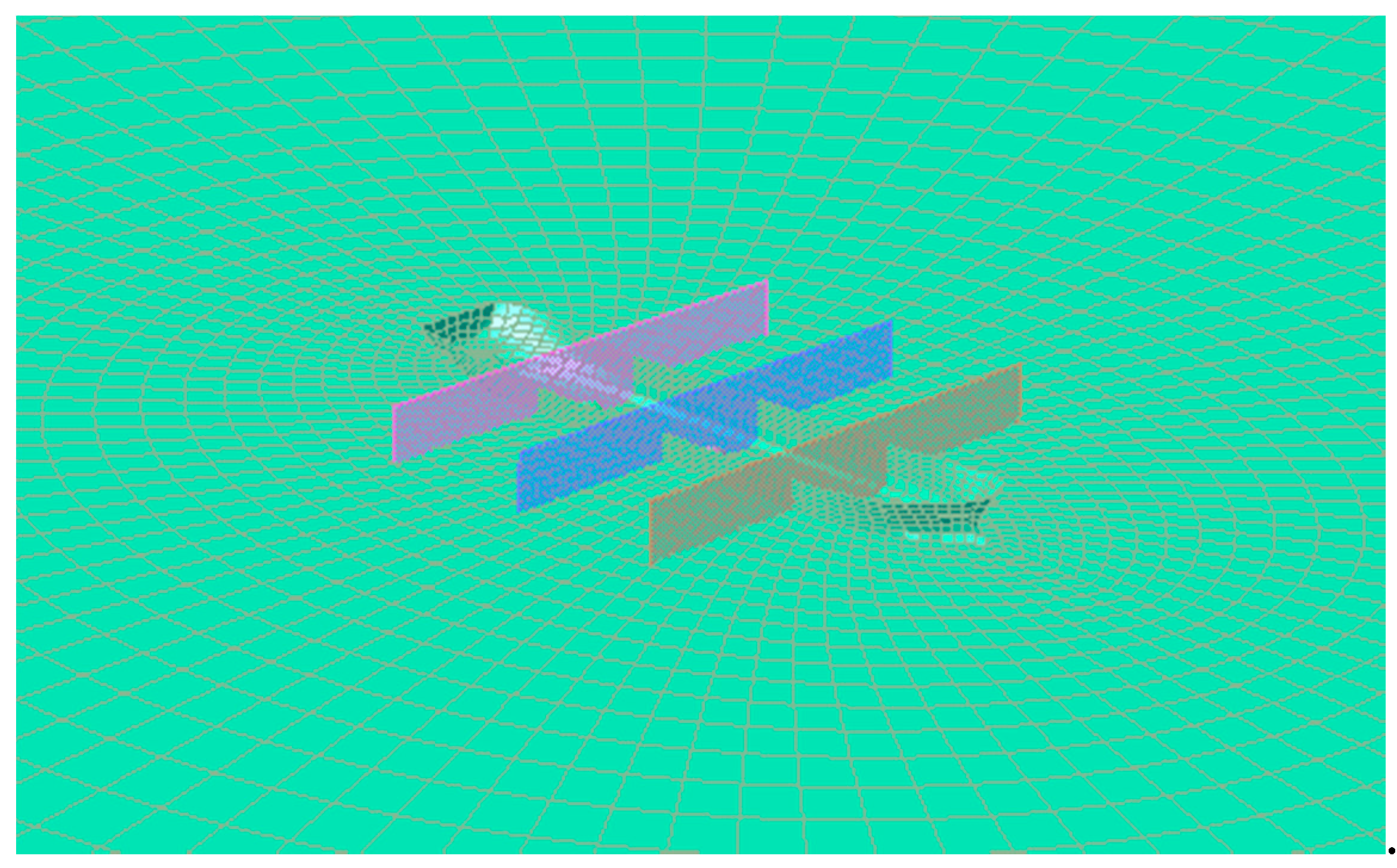
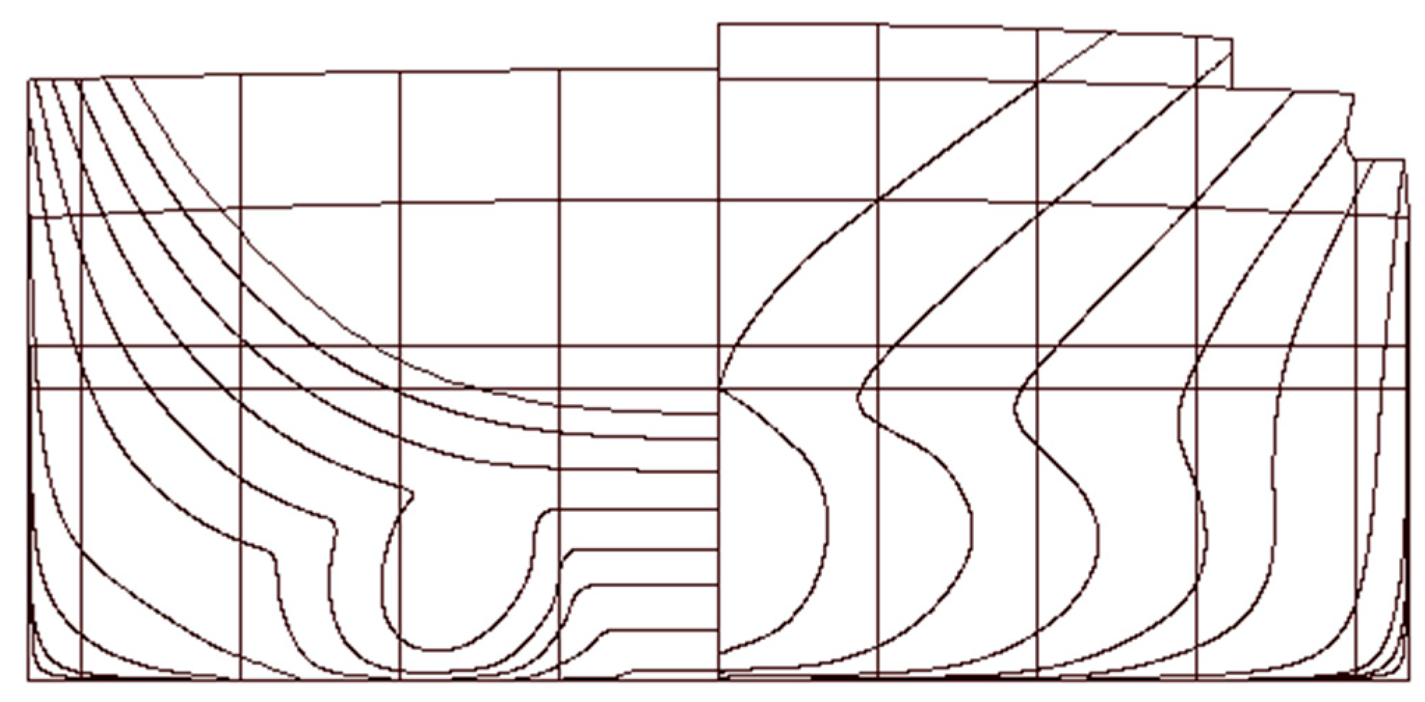
The mesh of the ship and the free surface in HydroD-Wasim are shown in Figure 8. Approximately 86 panels are generated in the longitudinal hull direction, while there are 34 panels along the transverse direction. The free surface meshes are generated with a radius about 10 times the ship length. The body nonlinearity is accounted for by HydroD-Wasim. Beyond that, the Froude–Krylov and restoring hydrostatic forces are solved up to the instantaneous wetted surface considered in the nonlinear effects. However, the radiation and diffraction forces are linearized and calculated for the mean free surface, which means that the degree of the nonlinearity of Wasim is only partial.

In the hydroelastic time domain numerical simulations, the ship is modelled with 20 sections. Based on Froude scaling, the bending modulus E is scaled with $\lambda$, and the area moment of inertia is scaled as ${\lambda }^4$, where $\lambda$ is the Froude scale. Similarly, the shear rigidity $kGA$ was scaled as ${\lambda }^3$, where $k$ is the shear correction factor, which was taken as 5/6, $G$ is the shear modulus, and A is the cross sectional area of the structure. Figure 9 shows the distribution of the mass (ship’s scale) used in the finite element model, in which the structure was assumed to be a 2D non-uniform Timoshenko beam.

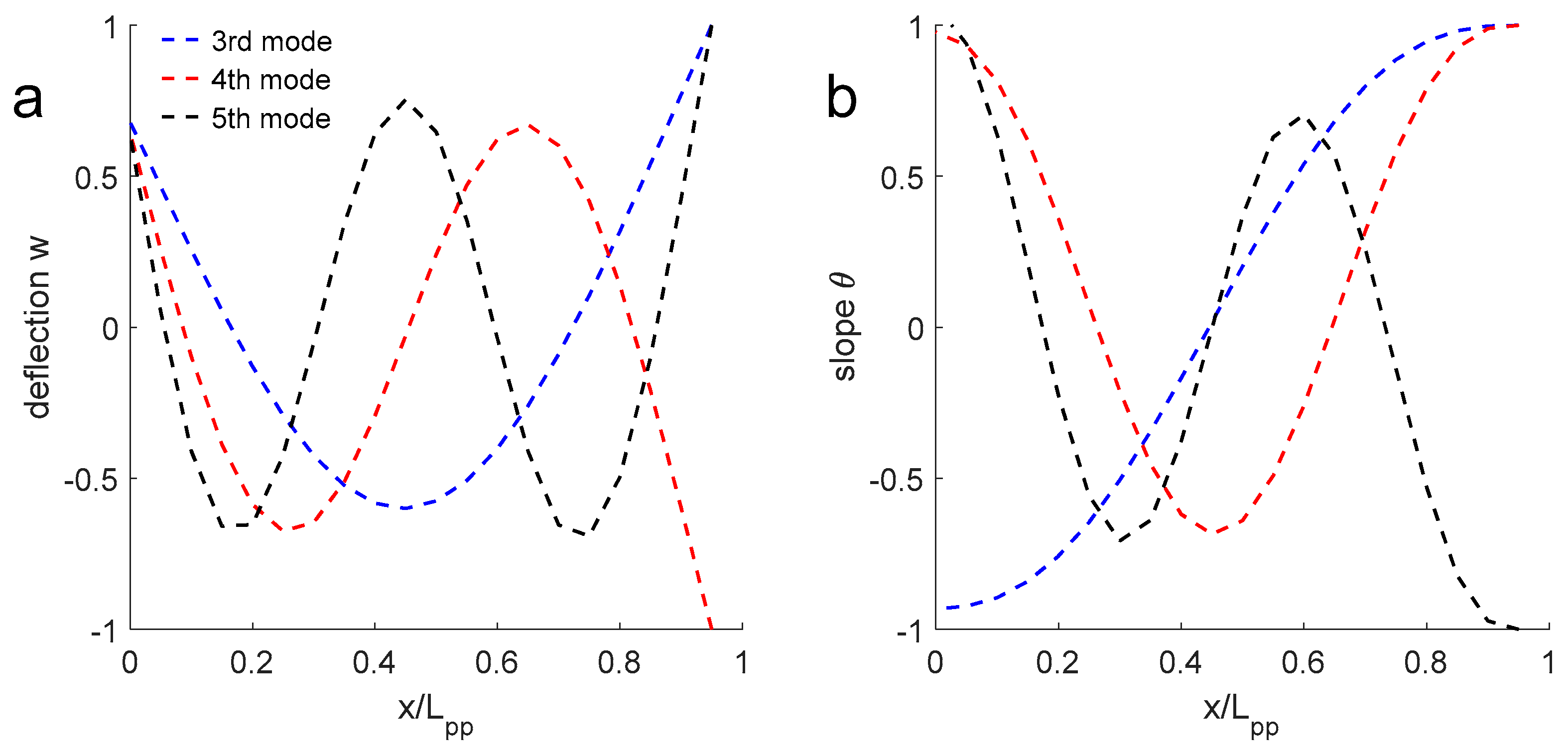
The exact calculation of the structural damping is complicated; therefore, the damping is assumed to be a linear combination of the mass and stiffness matrices. The critical damping ratio is chosen as 2.7% according to the free decay test results. The deflections and slopes up to third flexible modes for the ship calculated by the modal superposition analysis are presented in Figure 10, and the wet natural frequencies calculated for the flexible model are in good agreement with the measured values as shown in

Table 4. The wet natural vertical bending frequency of the ship (rad/s).

Mode	Experiment	Numerical
f2-nod	6.25	6.39
f3-nod	14.84	15.72
f4-nod	22.78	24.08

, even though the numerical results were slightly overestimated. There is good agreement between the measured and the numerical values for the lower modes; however, the disparity increases for higher modes. The wet natural frequency of the two-node vertical bending moment occurred at 6.25 and 6.39 rad/s in the experiment and numerical calculation, respectively.

5. Results

In this section, the experimental results measured in the wave tank and the numerical results are analysed and compared. The numerical results are represented by the acronyms “Htd” and “HydroD” in the following sections to denote the values numerically calculated by the hydroelastic time domain method and the software of HydroD-Wasim, respectively. The acronym “Exp” shows the experimental results.

5.1. RAOs (Response Amplitude Operators) of Vertical Responses

The RAOs of the vertical ship responses are analysed for the validation of the extended hydroelastic time domain method. The numerical and the experimental vertical response RAOs are given in Figure 11 against the encounter frequency. The numerical results include the hydroelastic time domain results and the Rankine panel method results. The plots on the left and right illustrate the ship responses with speeds of 10 and 14 knots, which correspond to Froude numbers of 0.144 and 0.202, respectively.

The heave RAOs from the two methods of numerical calculations match reasonably well with the experimental results, especially for the middle frequency range. However, the heave responses at the high frequencies are lower than the measurements for the Froude number of 0.202. As the incident waves become steeper, the discrepancy becomes more noticeable due to stronger nonlinearity. Strip theory predicts lower heave amplitudes than the panel code, except at very low frequencies.

The results of the pitch RAOs show a similar trend against the encounter frequency, although both numerical results are a bit lower than the test results. However, with the increase in speed, the RAOs of the pitch were reduced.

The non-dimensional VBM reach its peak value for all these three results when the ratio of the wave length to the ship’s perpendicular length is around 1.1 at both speeds. Moreover, with the increase in speed, the RAOs are enhanced as well, which is similar to the heave responses. The HydroD, implementing the Rankine panel method, overestimated the responses remarkably, while the hydroelastic numerical method coincided with the experimental results, even if there was still a slight discrepancy at the higher speed. Therefore, from a practical point of view, the hydroelastic time domain method provides a compromise between efficiency and accuracy, which is essential, especially during the design stage.

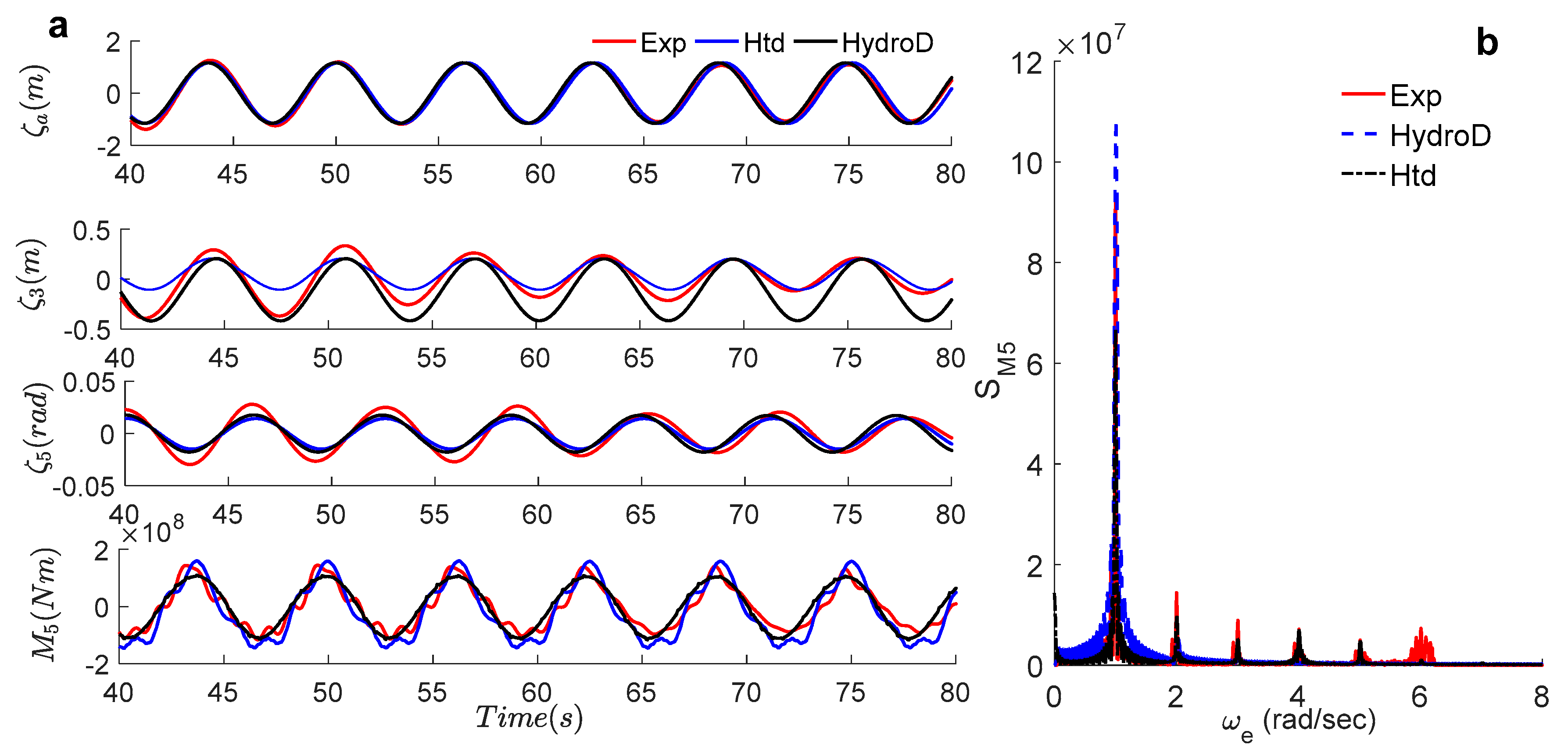
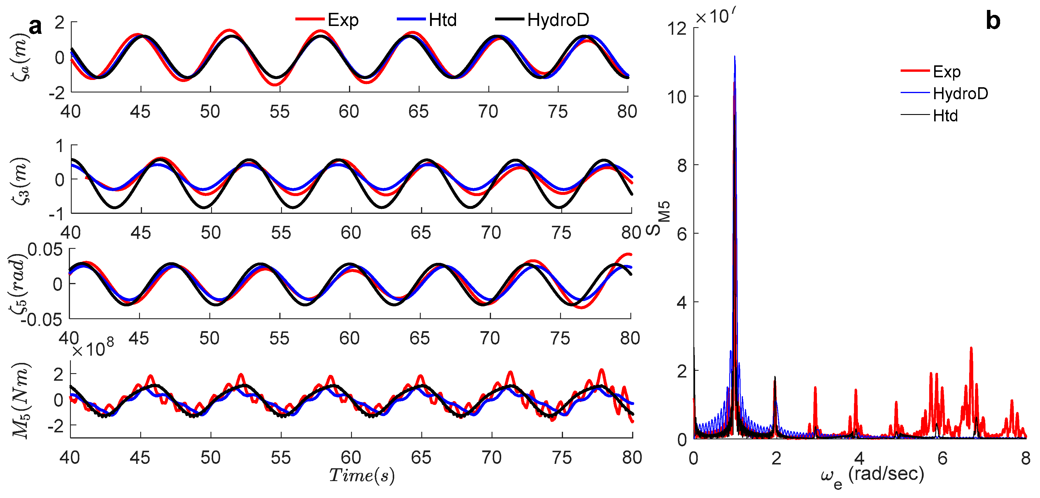
5.2. Comparison of Time and Frequency Domain Responses

The time series and spectral density of the measured data and numerical values at each speed are compared in Figure 12 to Figure 13 separately, and they present satisfactory agreement. Both the heave and pitch values are derived at the centre of mass, while the vertical bending moment corresponds to amidships.

The heave values obtained from HydroD are greater than the hydroelastic simulations and the measurements in these two regular waves at both speeds. It is obvious that the difference in heave for the wave-to-ship length of 0.9 is higher than the other, from the comparison shown in Figure 11. At same time, pitch shows more consistency among these three results. Meanwhile, with the increase in the encounter frequency resulting from the speed effect, the amplitudes of the motions are also increased, and they show a slight nonlinearity. The discrepancies among these three results are even higher in Case 3 compared to Case 2.

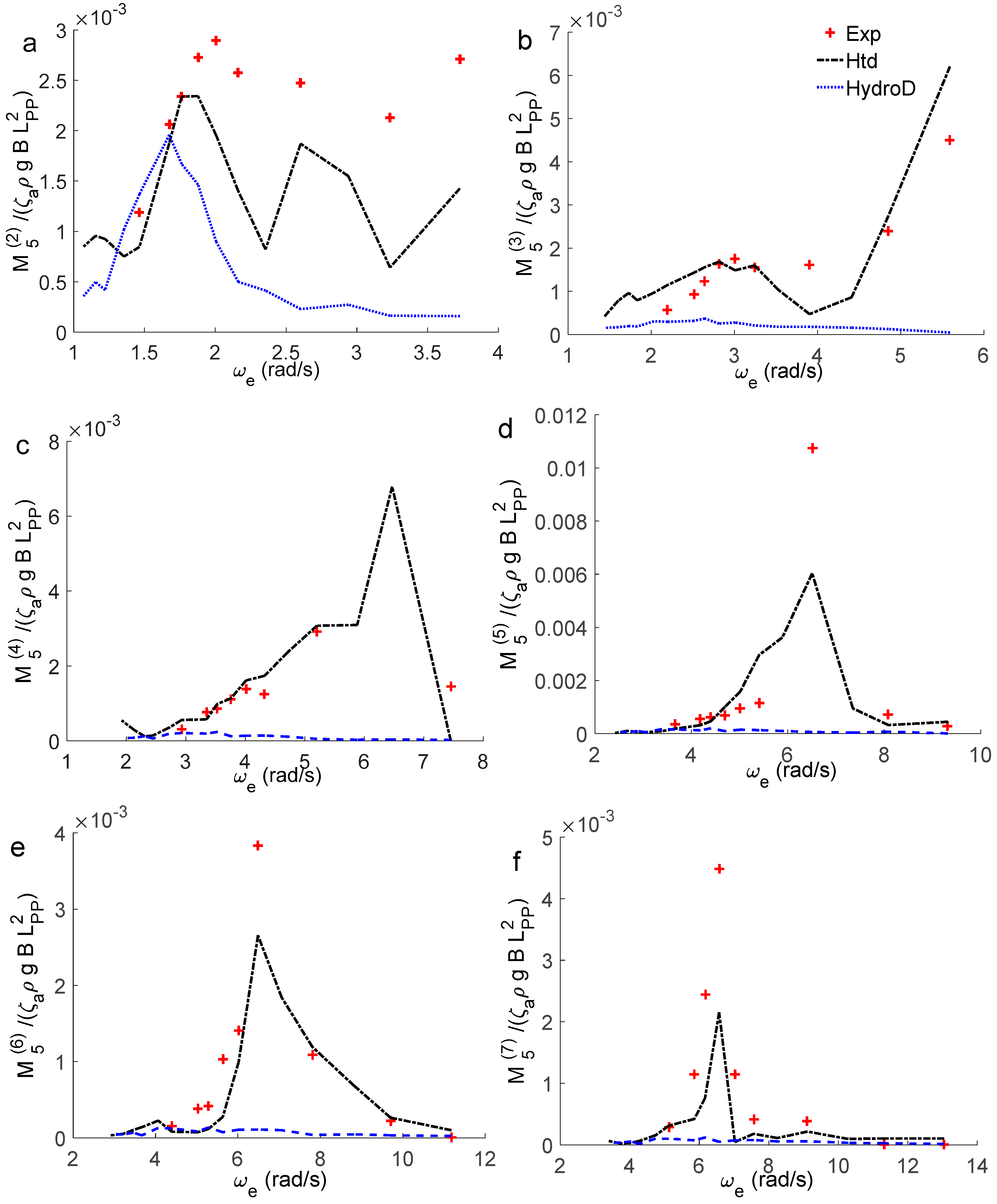
5.3. High-Order Harmonics of Ship Responses

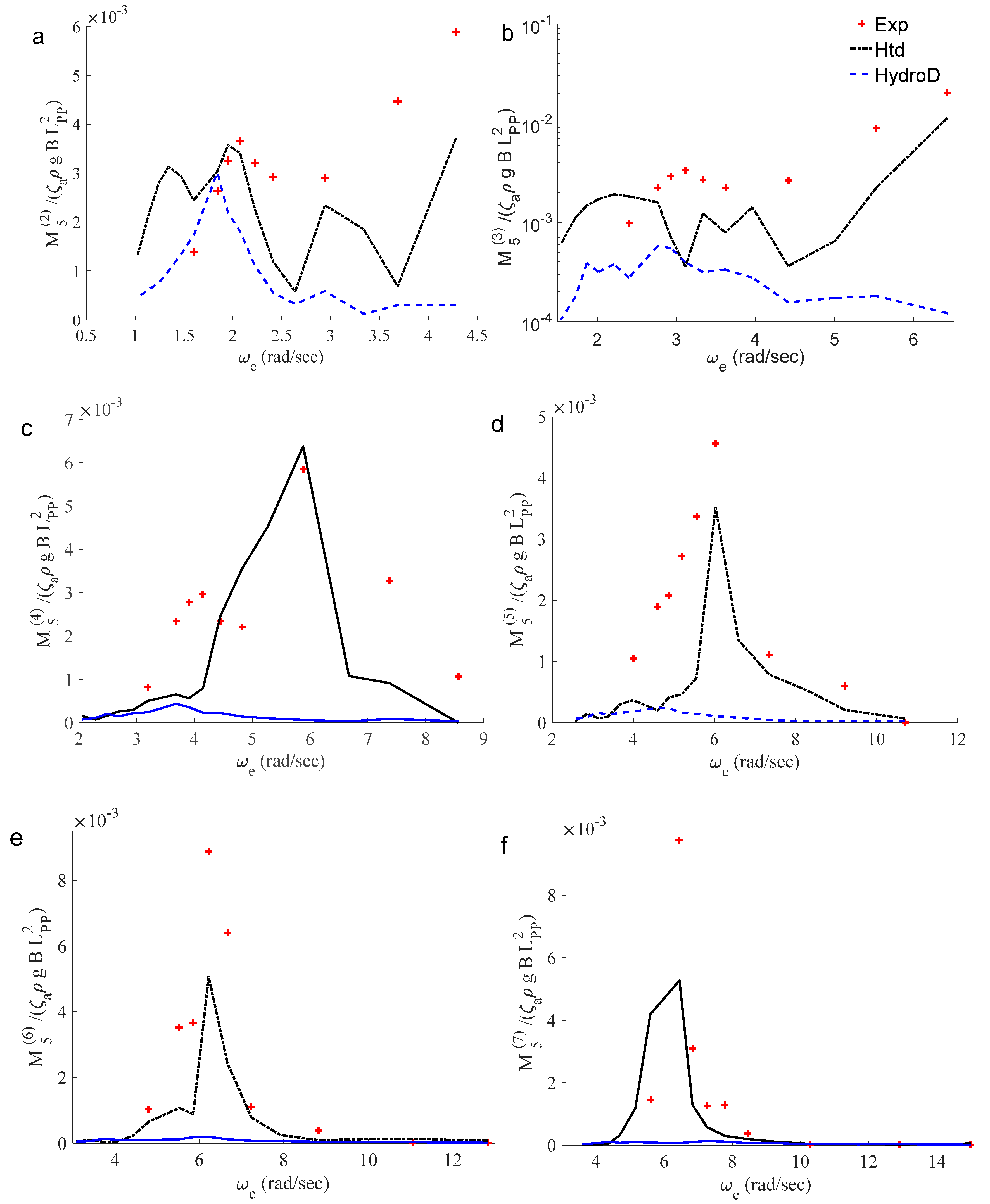
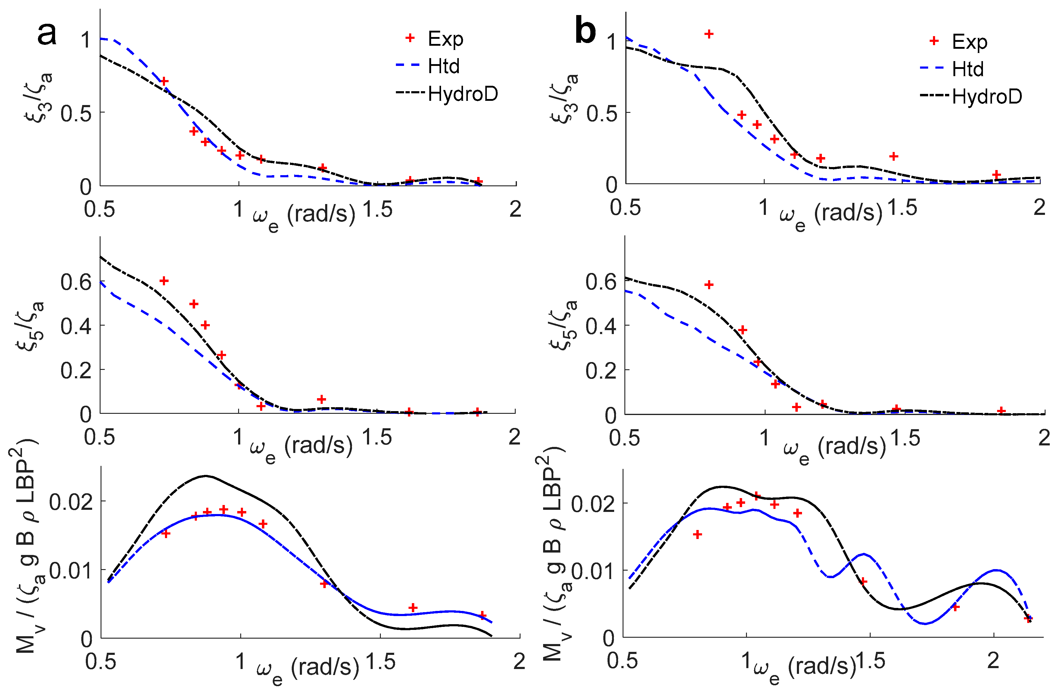
The comparisons between the high-order harmonics of the numerical and experimental VBM up to the seventh order with Froude numbers of 0.144 and 0.202 are shown in Figure 14; Figure 15, respectively. The black lines show the nonlinear hydroelastic time domain calculations, while the blue lines are extracted from HydroD.

The first order of the harmonics under several encounter frequencies has already been illustrated in Figure 11. The high-order harmonics are normally around 10% of the first harmonics, especially at a low-encounter frequency, avoiding the vicinity where the wet natural frequencies dominate. It should be noted that normally, the harmonics around the natural wet frequency of the model rise dramatically due to the amplifying effect of the springing vibration, which amounts to 31% of the first ones. The nonlinear hydroelastic time domain method is able to simulate the springing with such a strong nonlinear effect. However, even though it captured the high-order harmonics’ characteristics, the amplified value still underestimated the test results.

There is a large discrepancy in the sixth and seventh harmonics only when the encounter frequency is around the natural frequency of the model, but away from that frequency, the agreement is fine. The discrepancy being only at the natural frequency reflects some difficulty in the estimation of the corresponding damping, which is always very difficult for those high-order harmonics.

Along with the increase in speed, the second and third harmonics present similar trends with enlarged values. Again, the Rankine panel method could not identify the harmonics higher than the fourth order. The amplified peaks in the vicinity of the wetted natural frequency still show a distinct nonlinear in the high-order vibrations caused by the springing effects. Moreover, such effects are enhanced with the increase in the speed, while the wave heights do not change remarkably. The differences in the high-order harmonics of these two simulations are caused by several aspects.

Although HydroD-Wasim is a three-dimensional method, its nonlinearity is still simplified. The body nonlinearity is accounted for, the quadratic pressure is considered and the Froude–Krylov force and restoring forces are calculated up to the instantaneous wetted surfaces, but the radiation and diffraction forces are still linear and are solved on the mean free surface and mean wetted surface. Furthermore, the flexibility of the ship structure is not modelled, as it only takes into consideration the mass distribution and not the stiffness characteristics.

On the other hand, the nonlinear hydroelastic time domain code included the effect of slamming and green water forces as nonlinear loads. The nonlinear radiation force could account for the changes in the hull instantaneously wetted surface. The effect of the flexibility of the structure and the hydroelasticity on the ship responses is also modelled.

5.4. Slamming Loads and Their Occurrence

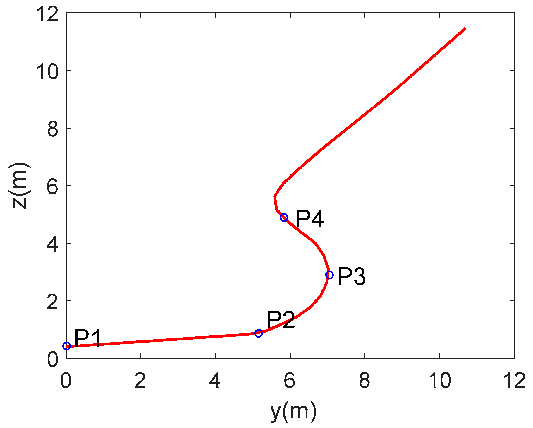
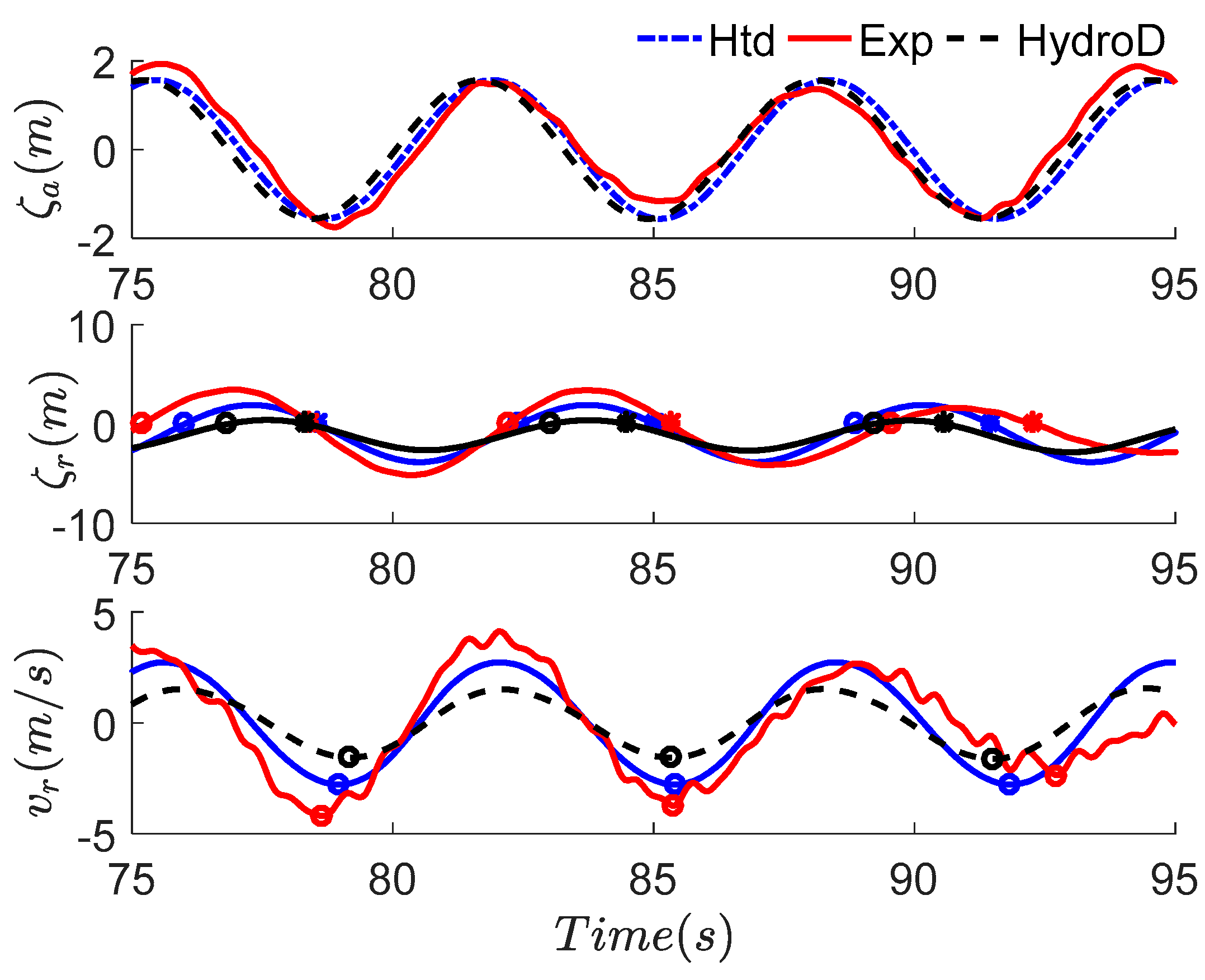
Since the slamming load depends very much on the deadrise angle, it is important to assess the slamming load for the river-to-sea ship’s cross sections with small deadrise angles. According to Section 3.5, the specific region in the bow where the slamming load occurs could be assessed. For instance, the relative motion and velocity of the location of P1 on Sta.19 are shown in Figure 16, as well as the wave elevation, while the cross section of Sta.19 and the slamming pressure location are presented in Figure 17.

The results are obtained by the hydroelastic time domain numerical simulation and by HydoD and compared with the experimental results, even though the HydroD had not taken into consideration the slamming loads. The estimated entry and exit points are marked in the curve of P1’s relative motion, with the $\lambda$ around the 1.1$L_{PP}$. Meanwhile, the peak velocity is also marked in the curve, which shows that the velocity reached its peak value just after the corresponding location of entry to the water.

It is shown that the measured impact velocities were larger than the prediction results. The calculated motion and velocity relative to the wave surface agree well with the measured results, except for a slight discrepancy for the peak and phase angle. The numerical results for the vertical velocity are lower than the measured ones. The simplifications used in the numerical method are one reason for the discrepancy in the relative motion. Beyond that, the wave elevation at the bow was transferred spatially according to the value at amidships utilizing linear dispersion. The bow slamming phenomena were recorded and are shown in Figure 18. During the slamming process, the bow of the ship model emerged from the water and impacted the water at a relatively high velocity. Under the influence of the slamming load, the nonlinearity of the motion and bending moment was more prominent. The flexible vibration was influenced by the slamming force, which in turn affected the hydrodynamic loads.

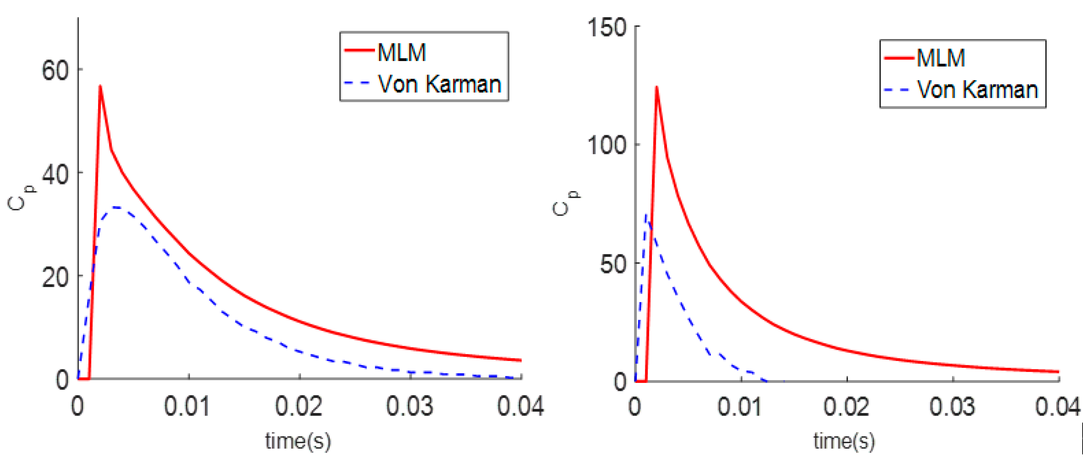
The measured slamming pressures on P1 were compared with the numerical and analytical calculation results shown in Figure 19. In the analytical calculation, the slamming pressure was obtained by the MLM model illustrated in Section 3.5. The numerical simulation was conducted with LS-DYNA, in which the impact velocity was the relative vertical velocity in the model tests at the same instants. The numerical modelling of the slamming problem was conducted by an Arbitrary-Lagrangian Eulerian (ALE) algorithm. The slamming event was simulated as a ship section impacting calm water. For an ALE solver, the fluid is solved using a Eulerian formulation, while the structure is discretized by a Lagrangian approach. A penalty coupling algorithm enables the interaction between the body and the fluids. The remap step in the ALE algorithm applies a Half-Index-Shift advection algorithm to update the fluid velocity and history variables. The interface between the solid structure and the fluids is captured by the Volume of Fluid method.

The MLM model results and numerical pressures are higher than the measured values. It is observed that the measured pressure includes an initial transient peak value and a relatively long duration with a lower amplitude of “momentum slamming”. The numerical results contain only the initial peak duration, while the MLM model results underestimate the “momentum slamming”. Due to the high beam/depth ratios of the geometry of the river-sea-going ship, the deadrise angle was relatively small. The time history of the slamming pressure shows that the “momentum slamming”, as the later stage impact, is essential for this ship type. The results calculated by the MLM model for the slamming pressure proved to be reasonable. The differences between the test results and the numerical and analytical calculations are mainly due to the three-dimensional effects in the tests. Beyond that, the variation of the impact velocity and impact of the local angle between the incoming wave surface and ship section also matters in the pressure history for such a blunt body.

It is worth stressing at this stage that the analysis presented here modelled the hydroelastic behaviour of the ship hull but slamming forces were calculated on the assumption of locally rigid structure at the location where slamming occurs. Other formulations [40,41] have analysed the local hydroelastic response, which may be worth considering in further studies.

6. Conclusions

In this paper, the hydroelastic response of a river-sea-going ship is analysed experimentally and numerically. A segmented ship model with a U-shaped cross section backbone is tested to reproduce the wave-induced loads and motions. A hydroelastic time domain method is extended to include the Modified Longcinovich Model (MLM) for calculating the slamming loads in such a blunt ship section. The slamming load on the bow represented by the MLM model is compared with the LS-DYNA simulation and with measured values.

The RAOs of the vertical responses in regular waves shows a good agreement with the extended code, while the Rankine panel method for a rigid hull overestimated the first harmonics slightly. Slight deviation is observed for a range of frequencies where large relative motions occur. Considering the high-frequency vibration effects such as springing, the Rankine panel’s results only show the second-order harmonics, while the hydroelastic simulations captures the amplified resonant vibrations consistent with the experiment’s high-frequency characteristics. The numerical simulation is able to capture the hydroelastic effect and represent nonlinear springing very well. The influence of springing on the vertical bending moment is significant and not negligible when the encounter frequency is in the vicinity of the first flexible wet natural frequency.

It necessary to pay attention to such high beam/depth ratios of the geometry of the river-sea-going ship when evaluating the slamming pressure. The slamming load results for the bow section of such a ship type calculated by the MLM model proved to be reasonable, and they show that the “momentum slamming”, at a later stage after the impact, is essential for this ship type.

References

1. Guedes Soares, C. Transient Response of Ship Hulls to Wave Impact. Int. Shipbuild. Prog. 1989, 36, 137–156. [Google Scholar]
2. Faltinsen, O.M. The effect of hydroelasticity on ship slamming. Philos. Trans. R. Soc. Lond. Ser. A 1997, 355, 575–591. [Google Scholar] [CrossRef]
3. Bishop, R.E.D.; Price, W.G. Hydroelasticity of Ships; Cambridge University Press: New York, NY, USA, 1979. [Google Scholar]
4. Santos, F.M.; Temarel, P.A.; Guedes Soares, C. On the Limitations of Two and Three-dimensional Linear Hydroelasticity Analyses Applied to a Fast Patrol Boat. J. Eng. Marit. Environ. 2009, 223, 457–478. [Google Scholar] [CrossRef]
5. Senjanović, I.; Malenica, S.; Tomasevic, S. Hydroelasticity of large container ships. Mar. Struct. 2009, 22, 287–314. [Google Scholar] [CrossRef]
6. Rajendran, S.; Fonseca, N.; Guedes Soares, C. A numerical investigation of the flexible vertical response of an Ultra Large Containership in high seas compared with experiments. Ocean Eng. 2016, 122, 293–310. [Google Scholar] [CrossRef]
7. Corak, M.; Parunov, J.; Guedes Soares, C. Long-term prediction of combined wave and whipping bending moments of containership. Ships Offshore Struct. 2015, 10, 4–19. [Google Scholar] [CrossRef]
8. Wang, Y.W.; Wu, W.G.; Guedes Soares, C. Experimental and numerical studies of the wave-induced responses of a River-Sea-Going ship. J. Mar. Sci. Appl. 2018, 17, 380–388. [Google Scholar] [CrossRef]
9. Fonseca, N.; Guedes Soares, C. Time domain analysis of large amplitude vertical motions and wave loads. J. Ship Res. 1998, 42, 100–113. [Google Scholar]
10. Fonseca, N.; Guedes Soares, C. Experimental investigation of the nonlinear effects on the vertical motions and loads of a containership in regular waves. J. Ship Res. 2004, 48, 118–147. [Google Scholar]
11. Fonseca, N.; Guedes Soares, C. Experimental investigation of the nonlinear effects on the statistics of vertical motions and loads of a containership in irregular waves. J. Ship Res. 2004, 48, 148–167. [Google Scholar]
12. Fonseca, N.; Pascoal, R.A.; Guedes Soares, C.; Clauss, G.; Schmitner, C. Numerical and experimental analysis of extreme wave induced vertical bending moments on a FPSO. Appl. Ocean Res. 2010, 32, 373–390. [Google Scholar] [CrossRef]
13. Rajendran, S.; Fonseca, N.; Guedes Soares, C. Simplified body nonlinear time domain calculation of vertical ship motions and wave loads in large amplitude waves. Ocean Eng. 2015, 107, 157–177. [Google Scholar] [CrossRef]
14. Rajendran, S.; Fonseca, N.; Guedes Soares, C. Body nonlinear time domain calculation of vertical ship responses in extreme seas accounting for 2nd order Froude-Krylov pressure. Appl. Ocean Res. 2016, 54, 39–52. [Google Scholar] [CrossRef]
15. Fonseca, N.; Antunes, E.; Guedes Soares, C. Whipping response of vessels with large amplitude motions. In Proceedings of the 25th International Conference on Offshore Mechanics and Arctic Engineering, Hamburg, Germany, 4–9 June 2006; Volume 92412. [Google Scholar]
16. Wagner, H. Uber Stossund Gleitvergange an der Oberflache von Flussigkeiten. Z. Angew. Math. Mech. 1932, 12, 193–215. [Google Scholar] [CrossRef]
17. Logvinovich, G.V. Hydrodynamics of Flows with Free Boundaries; Naukova Dumka: Kyiv, Ukaraine, 1973. [Google Scholar]
18. Korobkin, A.A. Analytical models of water impact. Eur. J. Appl. Math. 2004, 15, 821–838. [Google Scholar] [CrossRef]
19. Iijima, K.; Yao, T.; Moan, T. Structural responses of a ship in severe seas considering global hydroelastic vibration. Mar. Struct. 2008, 21, 420–445. [Google Scholar] [CrossRef]
20. Wu, M.K.; Moan, T. Linear and nonlinear hydroelastic analysis of high-speed vessels. J. Ship Res. 1996, 40, 149–163. [Google Scholar]
21. Zhu, S.; Wu, M.; Moan, T. Investigation into the nonlinear hydroelastic response of an 8600-TEU containership model advancing in regular waves. Ships Offshore Struct. 2014, 9, 74–87. [Google Scholar] [CrossRef]
22. Zhu, S.; Moan, T. New insight into the wave-induced nonlinear vertical load effects of ultra-large containerships based on experiments. J. Mar. Sci. Technol. 2013, 18, 87–114. [Google Scholar] [CrossRef]
23. Zhu, S.; Moan, T. Nonlinear effects from wave-induced maximum vertical bending moment on a flexible ultra-large containership model in severe head and oblique seas. Mar. Struct. 2014, 35, 1–15. [Google Scholar] [CrossRef]
24. Kim, K.H.; Bang, J.S.; Kim, J.H.; Kim, Y.; Kim, S.J.; Kim, Y. Fully coupled BEM-FEM analysis for ship hydroelasticity in waves. Mar. Struct. 2013, 33, 71–99. [Google Scholar] [CrossRef]
25. Datta, R.; Guedes Soares, C. Analysis of the hydroelastic effect on a container vessel using coupled BEM–FEM method in the time domain. Ships Offshore Struct. 2019, 2, 1–10. [Google Scholar] [CrossRef]
26. Hirdaris, S.E.; Price, W.G.; Temarel, P. Two- and three-dimensional hydroelastic analysis of a bulker in waves. Mar. Struct. 2003, 16, 627–658. [Google Scholar] [CrossRef]
27. Lakshmynarayanana, P.A.K.; Hirdaris, S. Comparison of nonlinear one- and two-way FFSI methods for the prediction of the symmetric response of a containership in waves. Ocean Eng. 2020, 203, 1–17. [Google Scholar] [CrossRef]
28. Wang, Y.W.; Wu, W.G.; Wang, S.; Guedes Soares, C. Slam-Induced Loads on a Three-Dimensional Bow with Various Pitch Angles. J. Offshore Mech. Arct. Eng. 2020, 142, 014502. [Google Scholar]
29. Sutulo, S.; Guedes Soares, C. A Boundary integral equations method for computing inertial and damping characteristics of arbitrary contours in deep fluid. Ship Technol. Res. 2004, 51, 69–93. [Google Scholar] [CrossRef]
30. Ramos, J.; Guedes Soares, C. On the assessment of hydrodynamic coefficients of cylinders in heaving. Ocean Eng. 1997, 24, 743–763. [Google Scholar] [CrossRef]
31. Frank, W. Oscillation of Cylinder in or below the Free Surface of Deep Fluids; Dept of Hydromechanics, David W Taylor Naval Ship Research and Development Centre: Bethesda, MD, USA, 1976. [Google Scholar]
32. Rajendran, S.; Vasquez, G.; Guedes Soares, C. Effect of bow flare on the vertical ship responses in abnormal waves and extreme seas. Ocean Eng. 2016, 124, 419–436. [Google Scholar] [CrossRef]
33. Wang, S.; Guedes Soares, C. Slam-induced loads on bow flared sections with various roll angles. Ocean Eng. 2013, 67, 45–57. [Google Scholar] [CrossRef]
34. Wang, S.; Guedes Soares, C. Experimental and numerical study of the slamming load on the bow of a chemical tanker in irregular waves. Ocean Eng. 2016, 111, 369–383. [Google Scholar] [CrossRef]
35. Wang, S.; Guedes Soares, C. Stern slamming of a chemical tanker in irregular head waves. Ocean Eng. 2016, 122, 322–332. [Google Scholar] [CrossRef]
36. Wang, S.; Zhang, H.D.; Guedes Soares, C. Slamming occurrence for a chemical tanker advancing in extreme waves modelled with the nonlinear Schrodinger equation. Ocean Eng. 2016, 119, 135–142. [Google Scholar] [CrossRef]
37. Wang, S. and Guedes Soares, C. Review of ship slamming loads and responses. J. Mar. Sci. Appl. 2017, 16, 427–445. [Google Scholar] [CrossRef]
38. Corak, M.; Parunov, J.; Guedes Soares, C. Probabilistic load combination factors of wave and whipping bending moments. J. Ship Res. 2015, 59, 11–30. [Google Scholar] [CrossRef]
39. Buchner, B. The Impact of Green Water on FPSO Design. In Proceedings of the Offshore Technology Conference, Houston, TX, USA, 1 May 1995; pp. 45–47. [Google Scholar]
40. Wang, S.; Karmakar, D.; Guedes Soares, C. Hydrodynamic impact of a horizontal floating plate with forward speed. J. Fluids Struct. 2016, 60, 97–113. [Google Scholar] [CrossRef]
41. Liu, B.; Wang, S.; Villavicencio, R.; Guedes Soares, C. Slamming load and hydroelastic structural response of bow flare areas of aluminium fast displacement crafts. Ocean Eng. 2020, 218, 108207. [Google Scholar] [CrossRef]
Figure 1. Body plan of the river-sea-going ship.
Jmse 08 00978 g001
Figure 2. Arrangement of segmented model and backbone.
Jmse 08 00978 g002
Figure 3. Section shape of backbone.
Jmse 08 00978 g003
Figure 4. Test model in the wave basin under regular waves.
Jmse 08 00978 g004
Figure 5. Hydrodynamic coefficients of the bow section.
Jmse 08 00978 g005
Figure 6. Geometry and fitting data of Sections A and B.
Jmse 08 00978 g006
Figure 7. Non-dimensional coefficients of slamming pressure on Sections A and B.
Jmse 08 00978 g007
Figure 8. Panel model in HydroD-Wasim.
Jmse 08 00978 g008
Figure 9. Mass distribution along the ship length.
Jmse 08 00978 g009
Figure 10. Wet natural frequency modes of the river-sea-going ship. (a) Deflection; (b) Slope.
Jmse 08 00978 g010
Figure 11. Experimental and numerical Response Amplitude Operators (RAOs) of the heave, pitch and vertical bending moments at amidship. (a) Fr = 0.144; (b) Fr = 0.202.
Jmse 08 00978 g011
Figure 12. Vertical response for λ / L = 0.9 of Fr = 0.144. (a) Time series of the wave elevation, heave, pitch and midship vertical bending moment. (b) Spectral density of the vertical bending moments.
Jmse 08 00978 g012
Figure 13. Vertical response for λ / L = 1.1 of Fr = 0.202. (a) Time series of the wave elevation, heave, pitch and midship vertical bending moment. (b) Spectral density of the vertical bending moments.
Jmse 08 00978 g013
Figure 14. Non-dimensional higher harmonics of the vertical bending moments up to 7th order at amidships in regular wave (Fr = 0.144). The plots (af) show the second to 7th harmonics, M5(2) to M5(7).
Jmse 08 00978 g014
Figure 15. Non-dimensional higher harmonics of the vertical bending moments up to 7th order at amidships in regular wave (Fr = 0.202). The plots (af) show the second to 7th harmonics, M5(2) to M5(7).
Jmse 08 00978 g015
Figure 16. Cross section of Sta.19 and location of the slamming pressure points.
Jmse 08 00978 g016
Figure 17. Wave elevation, relative vertical motion and corresponding impact velocities of P1’s location.
Jmse 08 00978 g017
Figure 18. Process of bow’s impact in the model test.
Jmse 08 00978 g018
Figure 19. Results for wave elevation, relative vertical motion and corresponding impact velocities of P1’s location in the condition of Case 4.
Jmse 08 00978 g019