Experimental Investigation of the Flow Field in the Vicinity of an Oscillating Wave Surge Converter


Abstract
:1. Introduction
2. Experimental Setup and Procedures
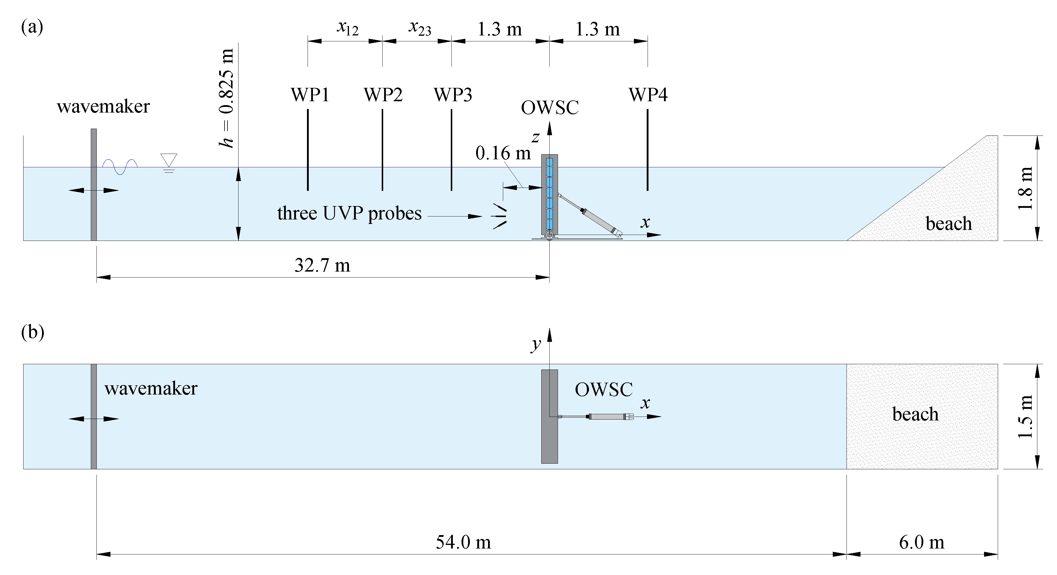
2.1. Wave Flume
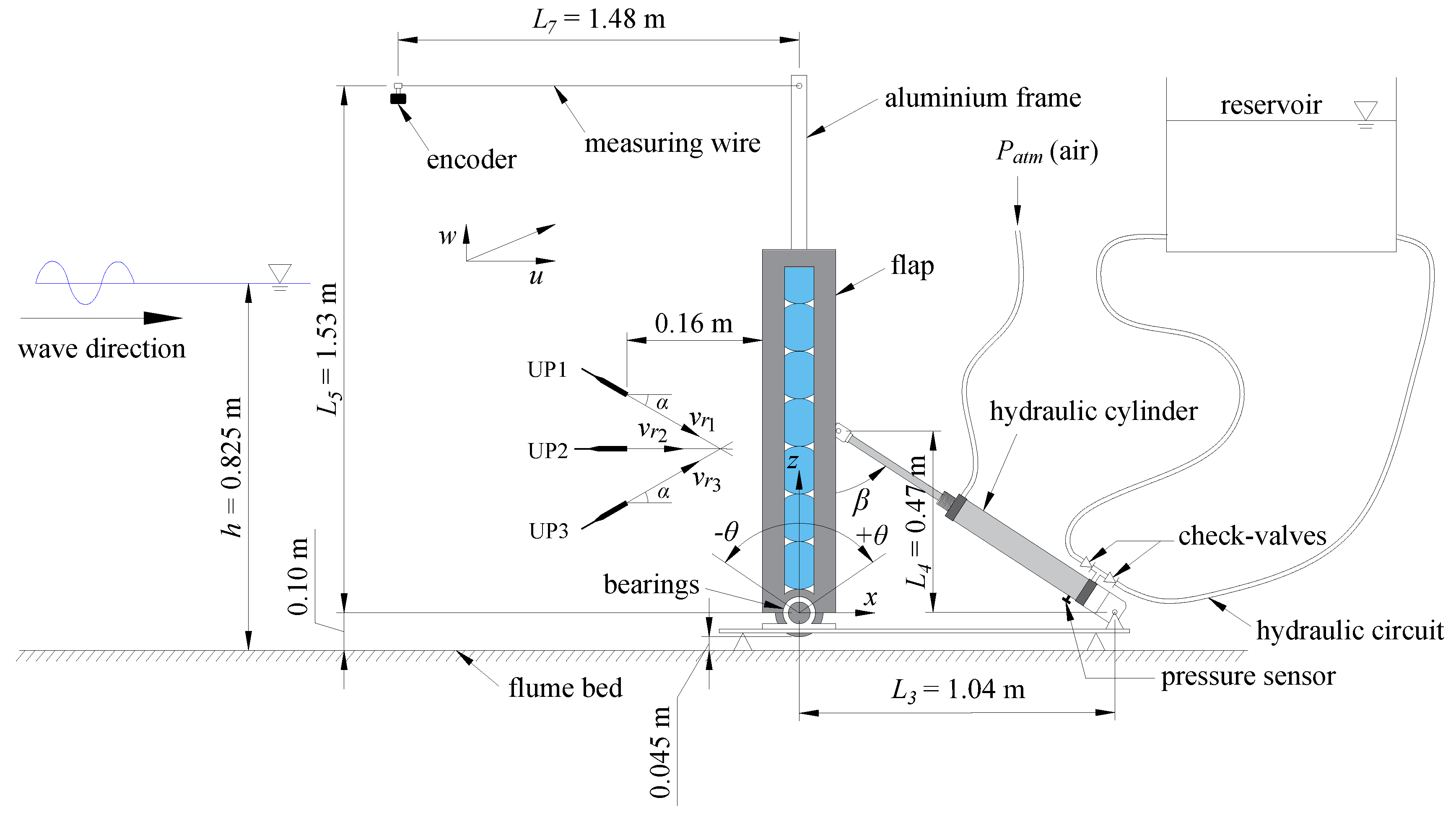
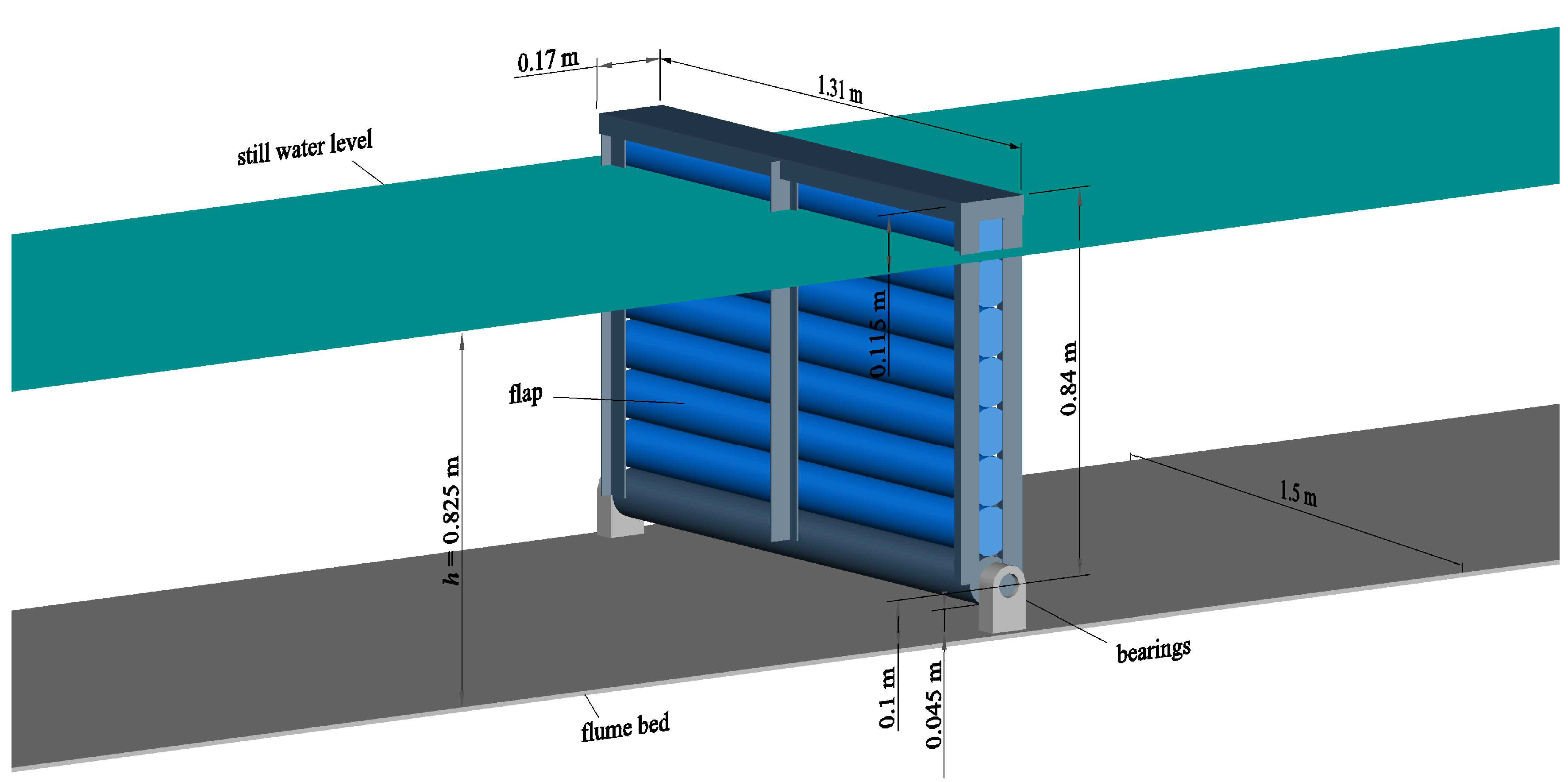
2.2. OWSC Model
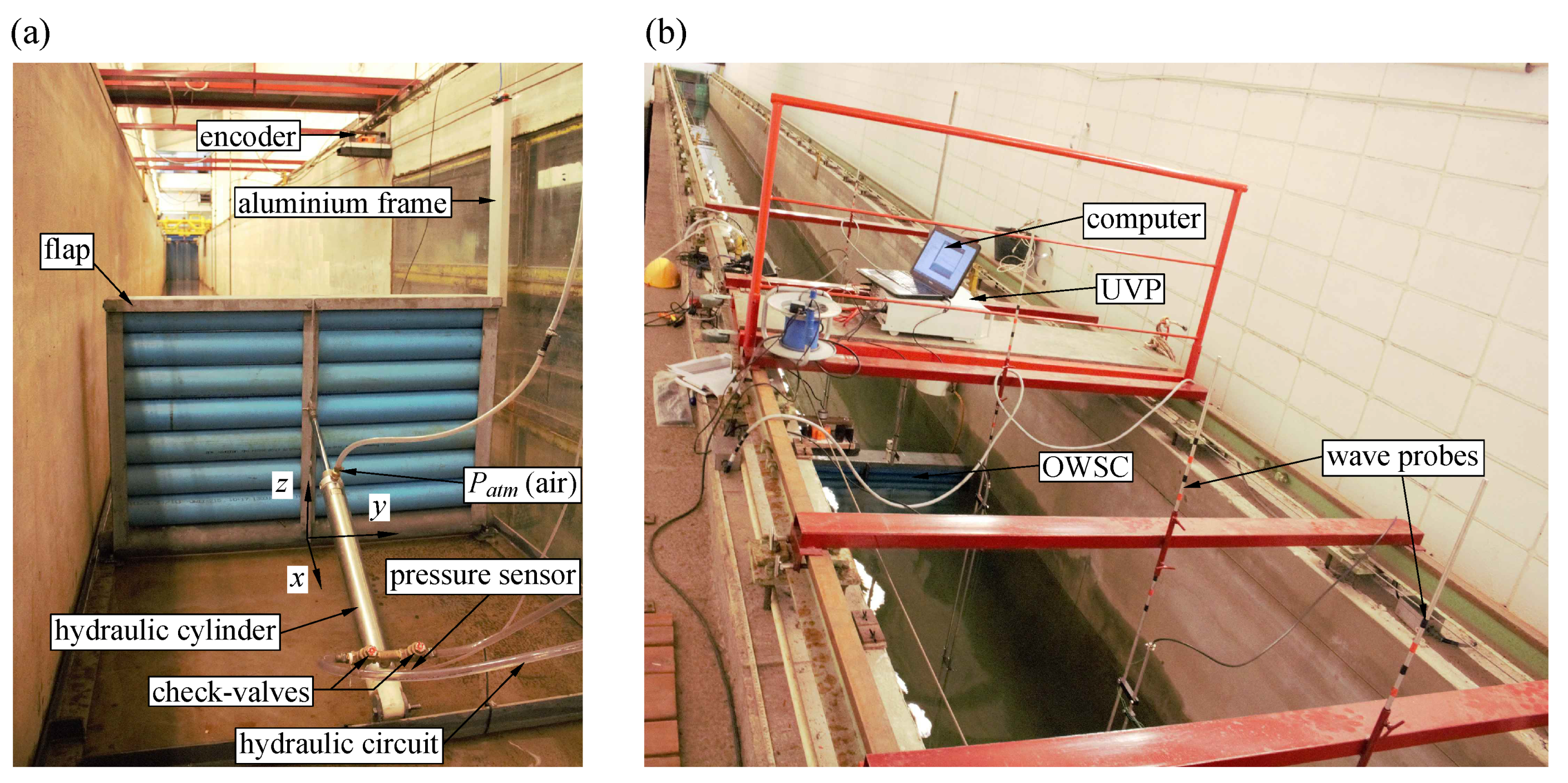
2.3. Full Experimental Setup and Instrumentation
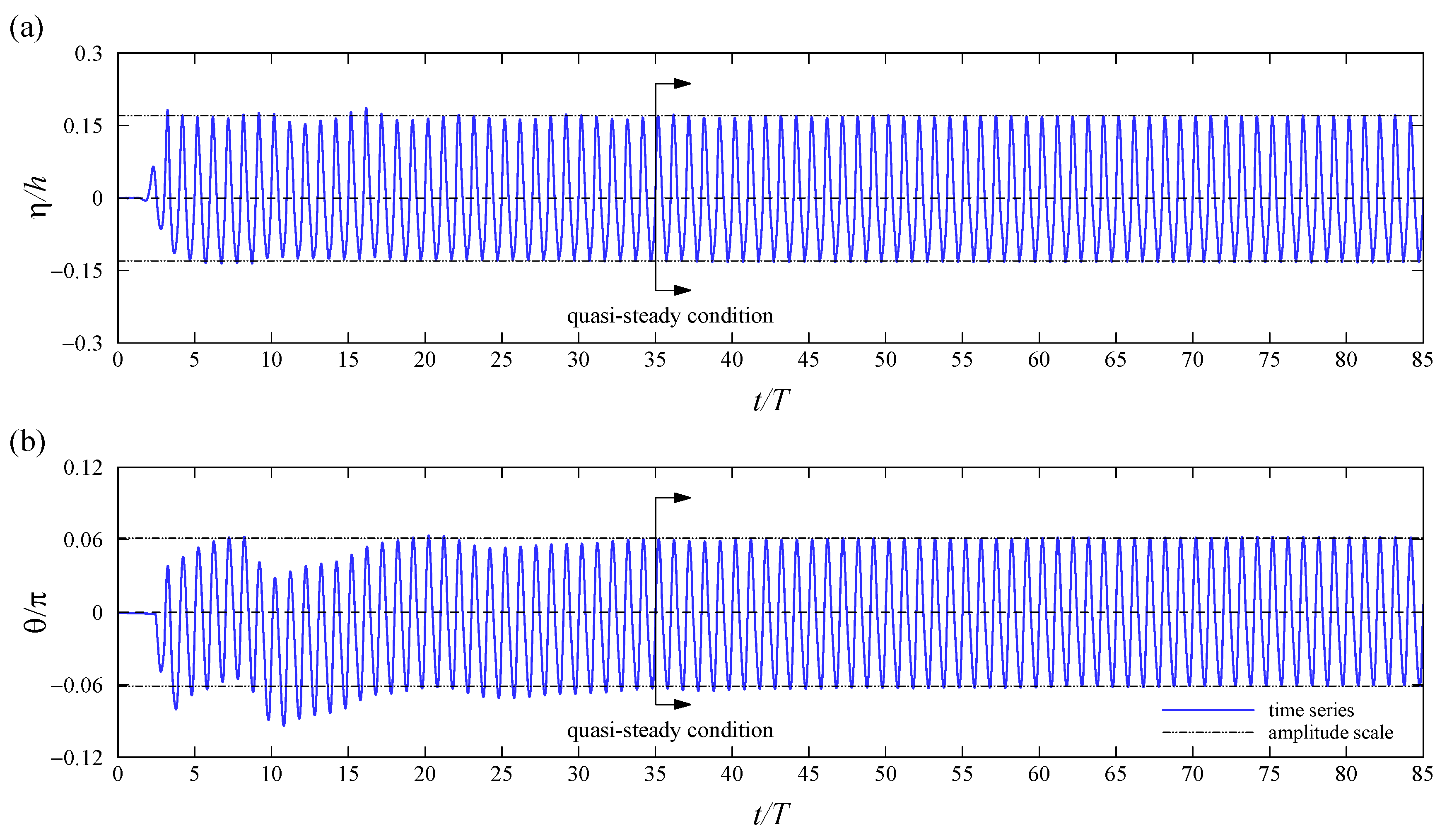
2.4. Data Collection
2.5. Repeatability of Experimental Tests
2.6. Data Analysis
3. Laboratory Evidence and Linear Wave Theory
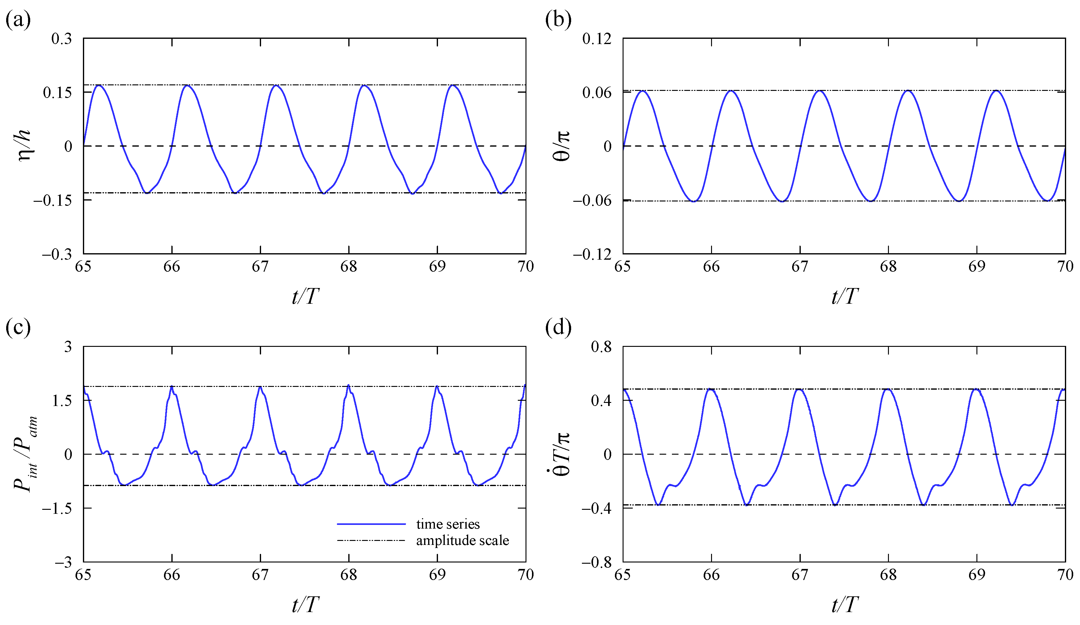
3.1. Dynamic Equilibrium
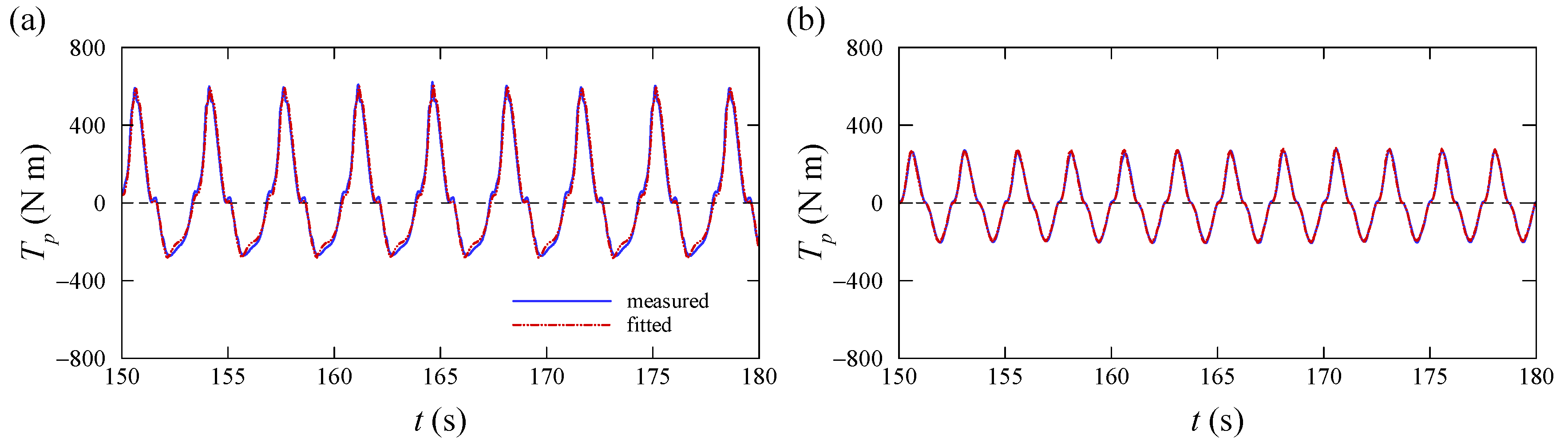
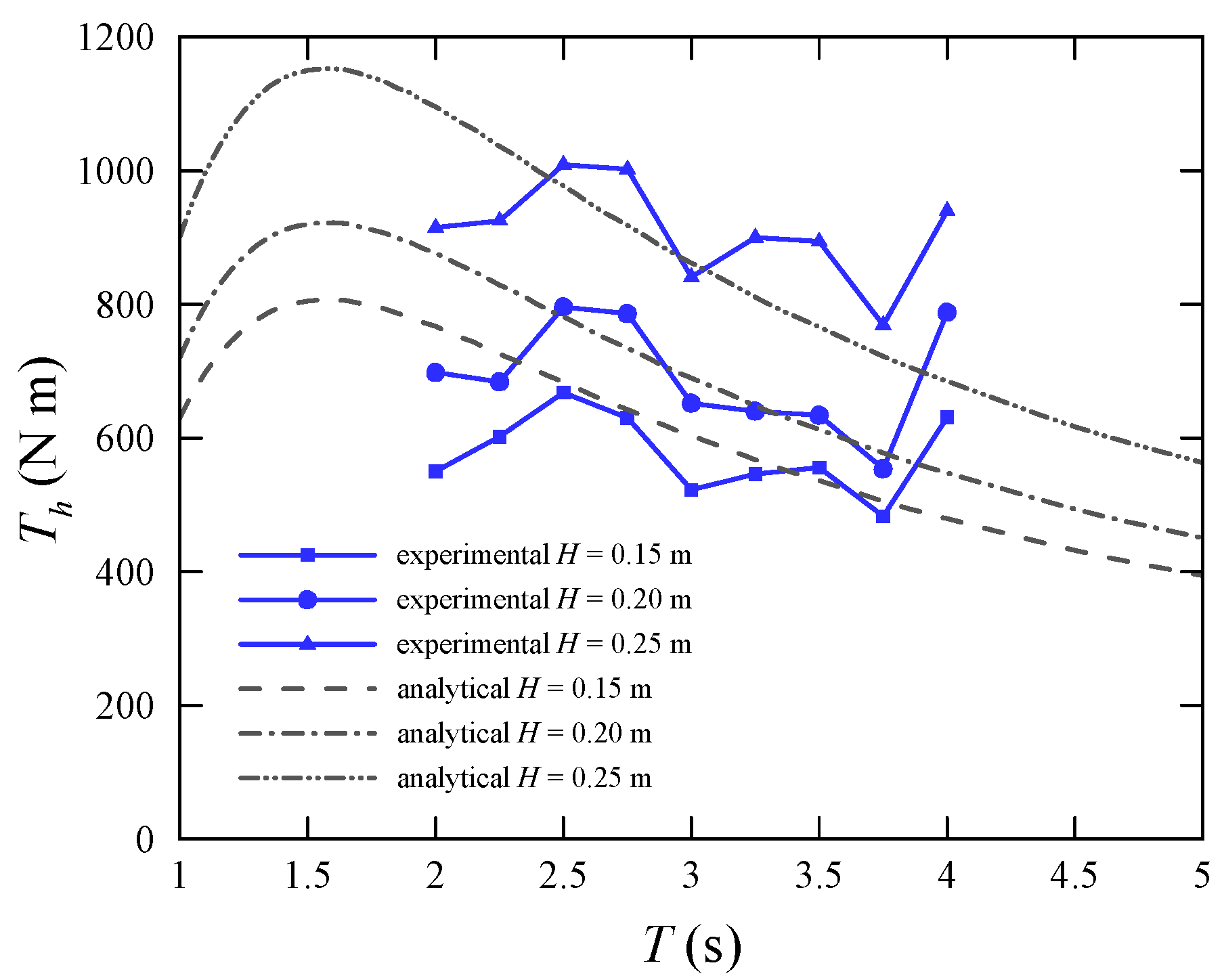
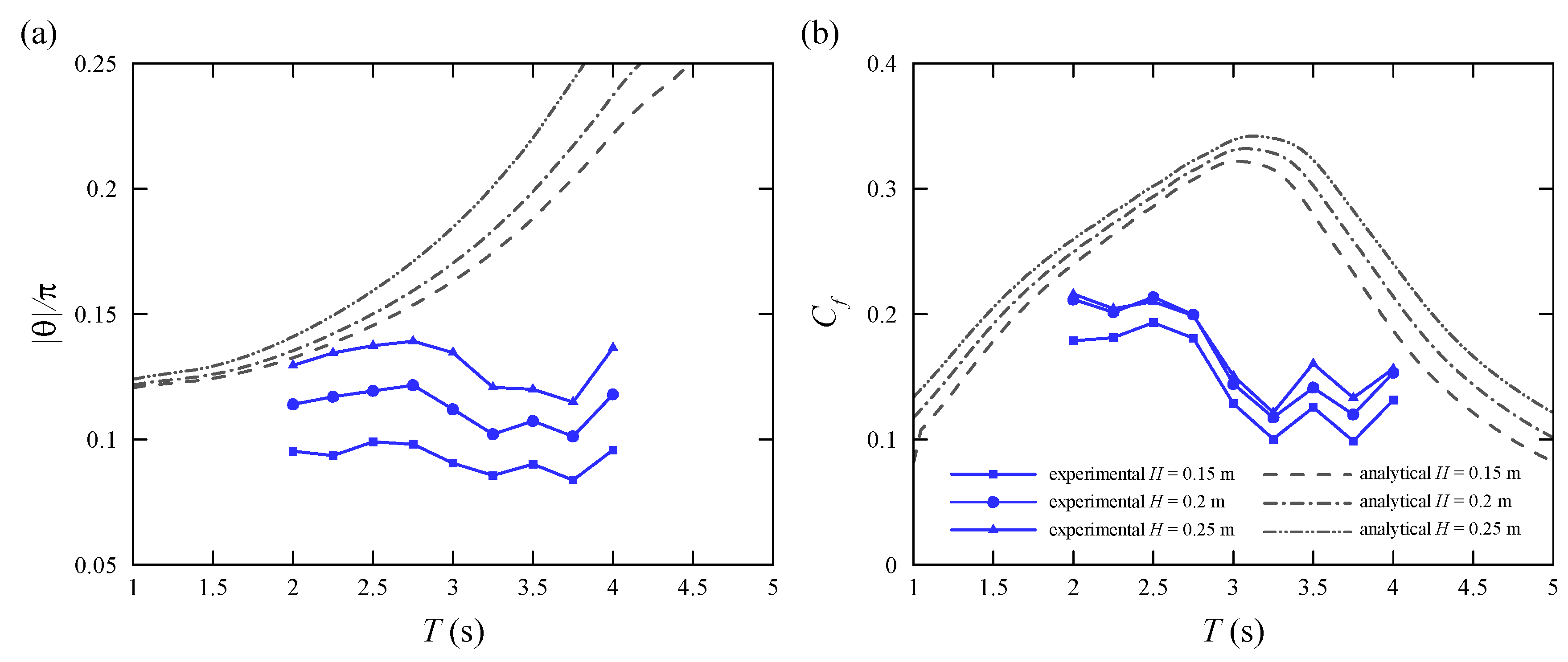
3.2. Hydrodynamic Torque: Experimental and Analytical Results
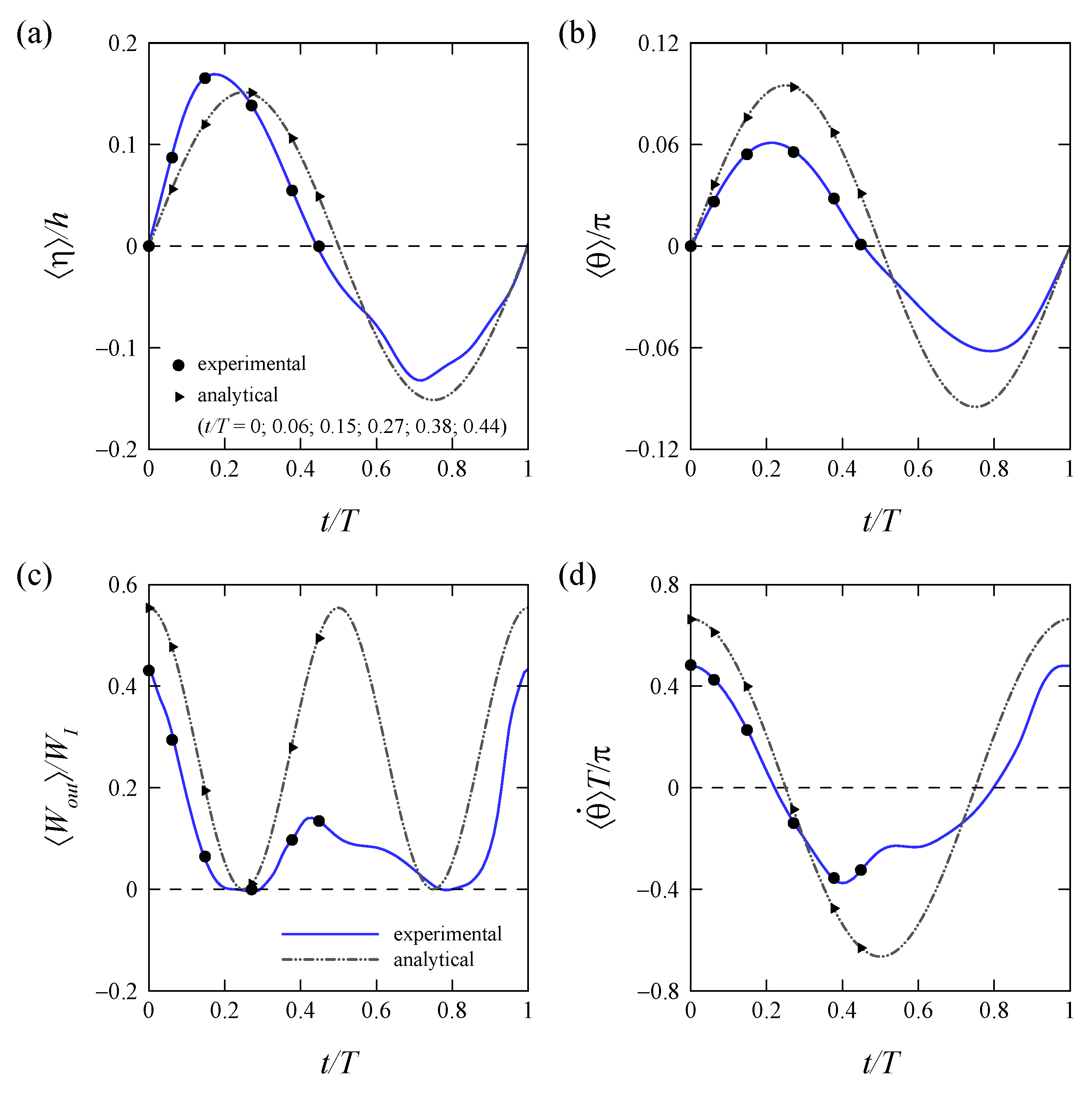
3.3. Dynamics of OWSC: Comparison between Experimental and Analytical Results
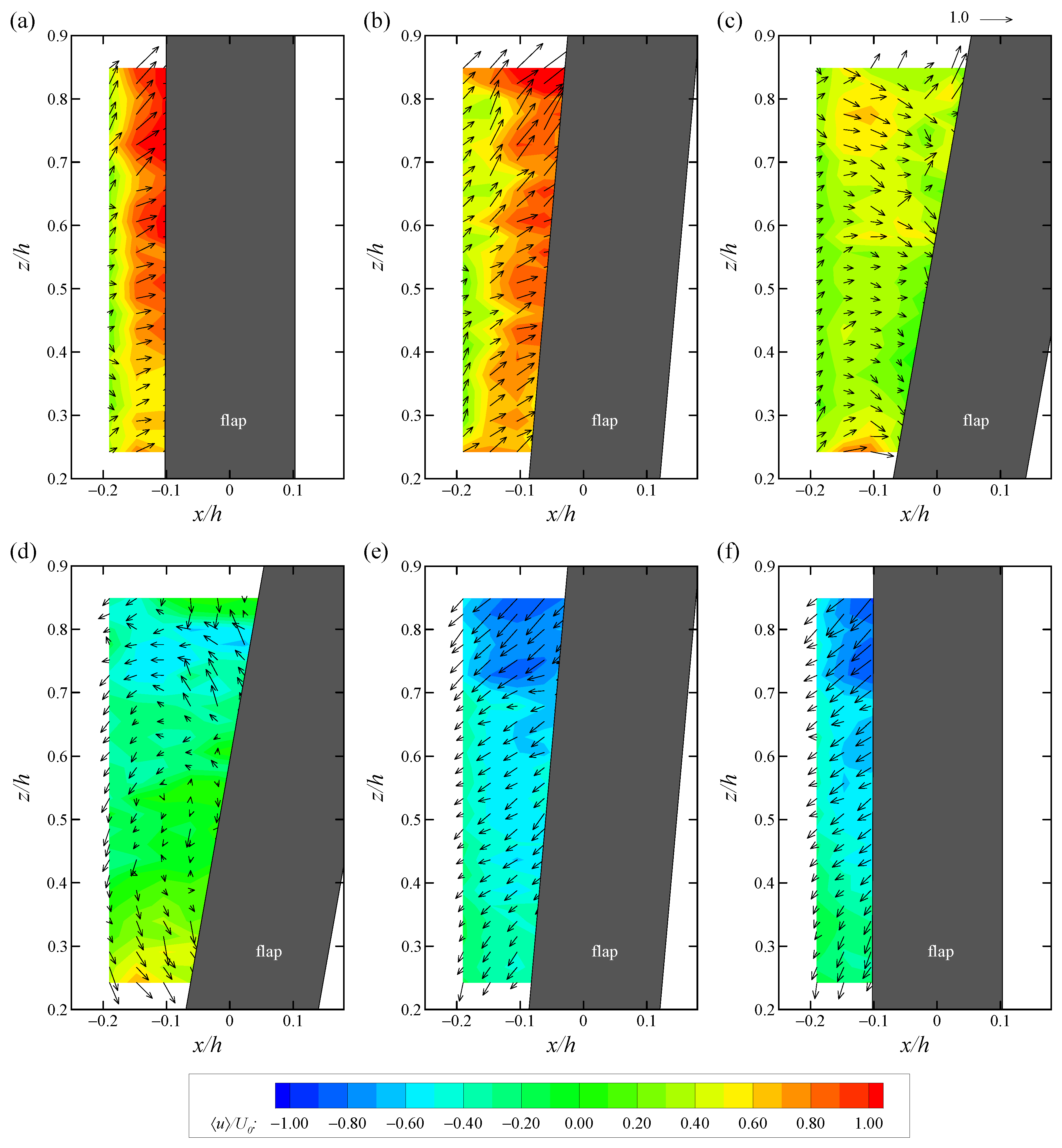
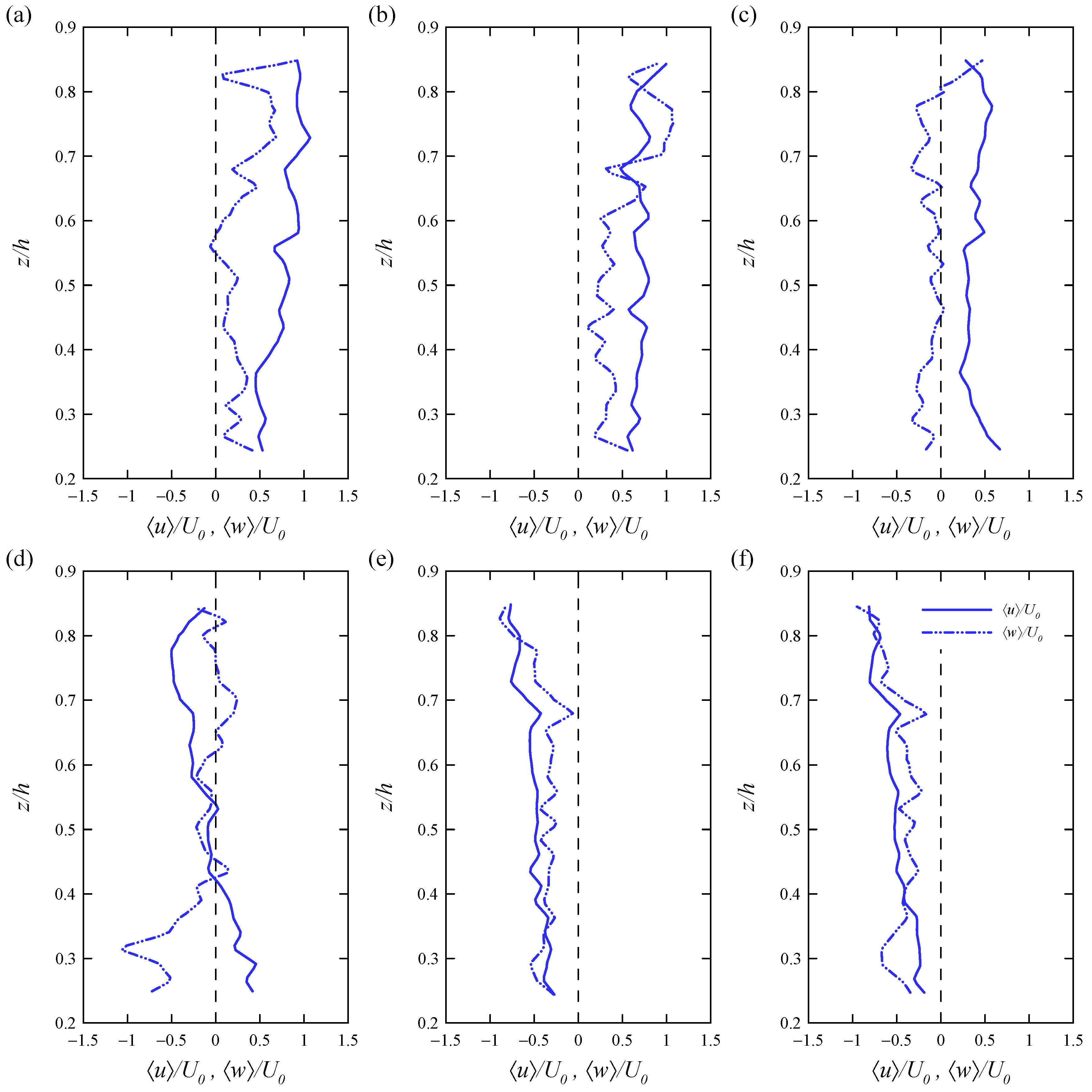
4. Mean and Turbulent Flow Field in Front of the OWSC
5. Conclusions
Author Contributions
Funding
Acknowledgments
Conflicts of Interest
Abbreviations
| OWSC | oscillating wave surge converter |
| PTO | power take-off |
| UVP | ultrasonic velocity profiler |
| WP | wave probe |
| UP | ultrasonic velocity profiler probe |
| RO | rated output |
| PPR | pulses per revolution |
Appendix A. Analytical Hydrodynamic Parameters
Appendix B. Friction Force Model
References
- Folley, M.; Whittaker, T.; Osterried, M. The Oscillating Wave Surge Converter. In Proceedings of the Fourteenth International Offshore and Polar Engineering Conference, Toulon, France, 23–28 May 2004. [Google Scholar]
- Whittaker, T.; Folley, M. Nearshore oscillating wave surge converters and the development of Oyster. Philos. Trans. R. Soc. Math. Phys. Eng. Sci. 2012, 370, 345–364. [Google Scholar] [CrossRef] [Green Version]
- Lucas, J.; Livingstone, M.; Vuorinen, N.; Cruz, J. Development of a wave energy converter (WEC) design tool—Application to the WaveRoller WEC including validation of numerical estimates. In Proceedings of the Fourth International Conference on Ocean Energy, Dublin, Ireland, 17 October 2012. [Google Scholar]
- Schmitt, P.; Asmuth, H.; Elsäßer, B. Optimising power take-off of an oscillating wave surge converter using high fidelity numerical simulations. Int. J. Mar. Energy 2016, 16, 196–208. [Google Scholar] [CrossRef] [Green Version]
- Renzi, E.; Doherty, K.; Henry, A.; Dias, F. How does Oyster work? The simple interpretation of Oyster mathematics. Eur. J. Mech.-B/Fluids 2014, 47, 124–131. [Google Scholar] [CrossRef] [Green Version]
- Whittaker, T.; Collier, D.; Folley, M.; Osterried, M.; Henry, A.; Crowley, M. The development of Oyster—A shallow water surging wave energy converter. In Proceedings of the 7th Annual European Wave & Tidal Energy Conference, Porto, Portugal, 11–13 September 2007. [Google Scholar]
- Brito, M.; Teixeira, L.; Canelas, R.B.; Ferreira, R.M.L.; Neves, M.G. Experimental and Numerical Studies of Dynamic Behaviors of a Hydraulic Power Take-Off Cylinder Using Spectral Representation Method. J. Tribol. 2017, 140, 021102. [Google Scholar] [CrossRef]
- Brito, M.; Ferreira, R.M.; Teixeira, L.; Neves, M.G.; Canelas, R.B. Experimental investigation on the power capture of an oscillating wave surge converter in unidirectional waves. Renew. Energy 2020, 151, 975–992. [Google Scholar] [CrossRef]
- Gomes, R.; Lopes, M.; Henriques, J.; Gato, L.; Falcão, A. The dynamics and power extraction of bottom-hinged plate wave energy converters in regular and irregular waves. Ocean. Eng. 2015, 96, 86–99. [Google Scholar] [CrossRef]
- Parsons, N.F.; Martin, P.A. Scattering of water waves by submerged plates using hypersingular integral equations. Appl. Ocean. Res. 1992, 14, 313–321. [Google Scholar] [CrossRef]
- Parsons, N.F.; Martin, P.A. Scattering of water waves by submerged curved plates and by surface-piercing flat plates. Appl. Ocean. Res. 1994, 16, 129–139. [Google Scholar] [CrossRef]
- Parsons, N.F.; Martin, P.A. Trapping of water waves by submerged plates using hypersingular integral equations. J. Fluid Mech. 1995, 284, 359. [Google Scholar] [CrossRef] [Green Version]
- Evans, D.; Porter, R. Hydrodynamic characteristics of a thin rolling plate in finite depth of water. Appl. Ocean. Res. 1996, 18, 215–228. [Google Scholar] [CrossRef]
- Renzi, E.; Dias, F. Resonant behavior of an oscillating wave energy converter in a channel. J. Fluid Mech. 2012, 701, 482–510. [Google Scholar] [CrossRef] [Green Version]
- Renzi, E.; Dias, F. Relations for a periodic array of flap-type wave energy converters. Appl. Ocean. Res. 2013, 39, 31–39. [Google Scholar] [CrossRef] [Green Version]
- Renzi, E.; Dias, F. Hydrodynamics of the oscillating wave surge converter in the open ocean. Eur. J. Mech.-B/Fluids 2013, 41, 1–10. [Google Scholar] [CrossRef] [Green Version]
- Falcão, A.F. Wave energy utilization: A review of the technologies. Renew. Sustain. Energy Rev. 2010, 14, 899–918. [Google Scholar] [CrossRef]
- Folley, M.; Whittaker, T.; Henry, A. The effect of water depth on the performance of a small surging wave energy converter. Ocean. Eng. 2007, 34, 1265–1274. [Google Scholar] [CrossRef]
- Henry, A. The Hydrodynamics of Small Seabed Mounted Bottom Hinged Wave Energy Converters in Shallow Water. Ph.D. Thesis, Queen’s University Belfast, Belfast, UK, 2009. [Google Scholar]
- Henry, A.; Folley, M.; Whittaker, T. A conceptual model of the hydrodynamics of an oscillating wave surge converter. Renew. Energy 2018, 118, 965–972. [Google Scholar] [CrossRef]
- Lin, C.C.; Chen, J.H.; Chow, Y.C.; Tzang, S.Y.; Hou, S.J.; Wang, F.Y. The Experimental Investigation of the Influencing Parameters of Flap Type Wave Energy Converters. In Proceedings of the 4th International Conference on Ocean Energy, Dublin, Ireland, 17–19 October 2012. [Google Scholar]
- Schmitt, P.; Bourdier, S.; Sarkar, D.; Renzi, E.; Dias, F.; Doherty, K.; Whittaker, T.; van’t Hoff, J. Hydrodynamic Loading on a Bottom Hinged Oscillating Wave Surge Converter. In Proceedings of the Twenty-second International Offshore and Polar Engineering Conference, Rhodes, Greece, 17–22 June 2012. [Google Scholar]
- Henry, A.; Kimmoun, O.; Nicholson, J.; Dupont, G.; Wei, Y.; Dias, F. A Two Dimensional Experimental Investigation of Slamming of an Oscillating Wave Surge Converter. In Proceedings of the Twenty-fourth International Ocean and Polar Engineering Conference, Busan, Korea, 15–20 June 2014. [Google Scholar]
- Henry, A.; Rafiee, A.; Schmitt, P.; Dias, F.; Whittaker, T. The Characteristics of Wave Impacts on an Oscillating Wave Surge Converter. J. Ocean. Wind. Energy 2014, 1, 101–110. [Google Scholar]
- Andersen, T.L.; Frigaard, P. Wave Generation in Physical Models: Technical Documentation for AwaSys 6; Department of Civil Engineering, Aalborg University: Aalborg, Denmark, 2014. [Google Scholar]
- Count, B.M.; Evans, D.V. The influence of projecting sidewalls on the hydrodynamic performance of wave-energy devices. J. Fluid Mech. 1984, 145, 361–376. [Google Scholar] [CrossRef]
- Mansard, E.; Funke, E. The Measurement of Incident and Reflected Spectra Using a Least Squares Method. In Coastal Engineering; American Society of Civil Engineers (ASCE): Reston, VA, USA, 1980. [Google Scholar] [CrossRef] [Green Version]
- Sarmento, A.J.N.A. Wave flume experiments on two-dimensional oscillating water column wave energy devices. Exp. Fluids 1992, 12, 286–292. [Google Scholar] [CrossRef]
- Met-Flow. UVP Monitor User’s Guide; Met-Flow S.A.: Lausanne, Switzerland, 2002. [Google Scholar]
- Lemmin, U.; Rolland, T. Acoustic Velocity Profiler for Laboratory and Field Studies. J. Hydraul. Eng. 1997, 123, 1089–1098. [Google Scholar] [CrossRef]
- Ting, F.C.; Kirby, J.T. Observation of undertow and turbulence in a laboratory surf zone. Coast. Eng. 1994, 24, 51–80. [Google Scholar] [CrossRef]
- Dimas, A.A.; Galani, K.A. Turbulent Flow Induced by Regular and Irregular Waves above a Steep Rock-Armored Slope. J. Waterw. Port Coastal Ocean. Eng. 2016, 142, 04016004. [Google Scholar] [CrossRef]
- Alonso, R.; Solari, S.; Teixeira, L. Wave energy resource assessment in Uruguay. Energy 2015, 93, 683–696. [Google Scholar] [CrossRef]
- Ting, F.C. Laboratory study of wave and turbulence velocities in a broad-banded irregular wave surf zone. Coast. Eng. 2001, 43, 183–208. [Google Scholar] [CrossRef]
- Van der A, D.A.; O’Donoghue, T.; Davies, A.G.; Ribberink, J.S. Experimental study of the turbulent boundary layer in acceleration-skewed oscillatory flow. J. Fluid Mech. 2011, 684, 251–283. [Google Scholar] [CrossRef] [Green Version]
- Monin, A.S.; Yaglom, A.M. Statistical Fluid Mechanics: Mechanics of Turbulence; MIT Press: Boston, MA, USA, 1971; Volume 1. [Google Scholar]
- Umeyama, M. Changes in Turbulent Flow Structure under Combined Wave-Current Motions. J. Waterw. Port Coastal Ocean. Eng. 2009, 135, 213–227. [Google Scholar] [CrossRef]
- Singh, S.K.; Debnath, K.; Mazumder, B.S. Turbulence Statistics of Wave-Current Flow over a Submerged Cube. J. Waterw. Port Coastal Ocean. Eng. 2016, 142, 04015027. [Google Scholar] [CrossRef]
- Yanada, H.; Sekikawa, Y. Modeling of dynamic behaviors of friction. Mechatronics 2008, 18, 330–339. [Google Scholar] [CrossRef]
- Tran, X.B.; Hafizah, N.; Yanada, H. Modeling of dynamic friction behaviors of hydraulic cylinders. Mechatronics 2012, 22, 65–75. [Google Scholar] [CrossRef]


| T (s) | H (m) | (m) | (m) |
|---|---|---|---|
| 2 | [0.15; 0.175; 0.2; 0.225; 0.25; 0.275; 0.3] | 0.49 | 1.23 |
| 2.25 | [0.15; 0.175; 0.2; 0.225; 0.25; 0.275; 0.3] | 0.57 | 1.42 |
| 2.5 | [0.15; 0.175; 0.2; 0.225; 0.25; 0.275; 0.3] | 0.65 | 1.62 |
| 2.75 | [0.15; 0.175; 0.2; 0.225; 0.25; 0.275; 0.3] | 0.72 | 1.81 |
| 3 | [0.15; 0.175; 0.2; 0.225; 0.25; 0.275; 0.3] | 0.8 | 2 |
| 3.25 | [0.15; 0.175; 0.2; 0.225; 0.25; 0.275; 0.3] | 0.88 | 2.19 |
| 3.5 | [0.15; 0.175; 0.2; 0.225; 0.25; 0.275; 0.3] | 0.95 | 2.38 |
| 3.75 | [0.15; 0.175; 0.2; 0.225; 0.25; 0.275; 0.3] | 1.02 | 2.56 |
| 4 | [0.15; 0.175; 0.2; 0.225; 0.25; 0.275; 0.3] | 1.1 | 2.75 |
Publisher’s Note: MDPI stays neutral with regard to jurisdictional claims in published maps and institutional affiliations. |
© 2020 by the authors. Licensee MDPI, Basel, Switzerland. This article is an open access article distributed under the terms and conditions of the Creative Commons Attribution (CC BY) license (http://creativecommons.org/licenses/by/4.0/).
Share and Cite
Brito, M.; Ferreira, R.M.L.; Teixeira, L.; Neves, M.G.; Gil, L. Experimental Investigation of the Flow Field in the Vicinity of an Oscillating Wave Surge Converter. J. Mar. Sci. Eng. 2020, 8, 976. https://doi.org/10.3390/jmse8120976
Brito M, Ferreira RML, Teixeira L, Neves MG, Gil L. Experimental Investigation of the Flow Field in the Vicinity of an Oscillating Wave Surge Converter. Journal of Marine Science and Engineering. 2020; 8(12):976. https://doi.org/10.3390/jmse8120976
Chicago/Turabian StyleBrito, Moisés, Rui M. L. Ferreira, Luis Teixeira, Maria G. Neves, and Luís Gil. 2020. "Experimental Investigation of the Flow Field in the Vicinity of an Oscillating Wave Surge Converter" Journal of Marine Science and Engineering 8, no. 12: 976. https://doi.org/10.3390/jmse8120976
APA StyleBrito, M., Ferreira, R. M. L., Teixeira, L., Neves, M. G., & Gil, L. (2020). Experimental Investigation of the Flow Field in the Vicinity of an Oscillating Wave Surge Converter. Journal of Marine Science and Engineering, 8(12), 976. https://doi.org/10.3390/jmse8120976