Evaluation of Pollutant Emissions into the Atmosphere during the Loading of Hydrocarbons in Marine Oil Tankers in the Arctic Region

Abstract

Emissions of volatile organic compounds into the atmosphere when loading oil or petroleum products into tankers are strong environmental pollutants. Given the increase in oil transport by sea and the development of Arctic routes, humanity faces the task of preserving the Arctic ecosystem. Vapor recovery units can limit the emissions of volatile organic compounds. However, it is necessary to estimate the emissions of oil and petroleum products vapors. This article offers two methods for estimating emissions of volatile organic compounds. In the analytical method, a mathematical model of evaporation dynamics and forecasting tank gas space pressure of the tanker is proposed. The model makes it possible to estimate the throughput capacity of existing gas phase discharge pipeline systems and is also suitable for designing new oil vapor recovery units. Creating an experimental laboratory stand is proposed in the experimental method, and its possible technological scheme is developed.

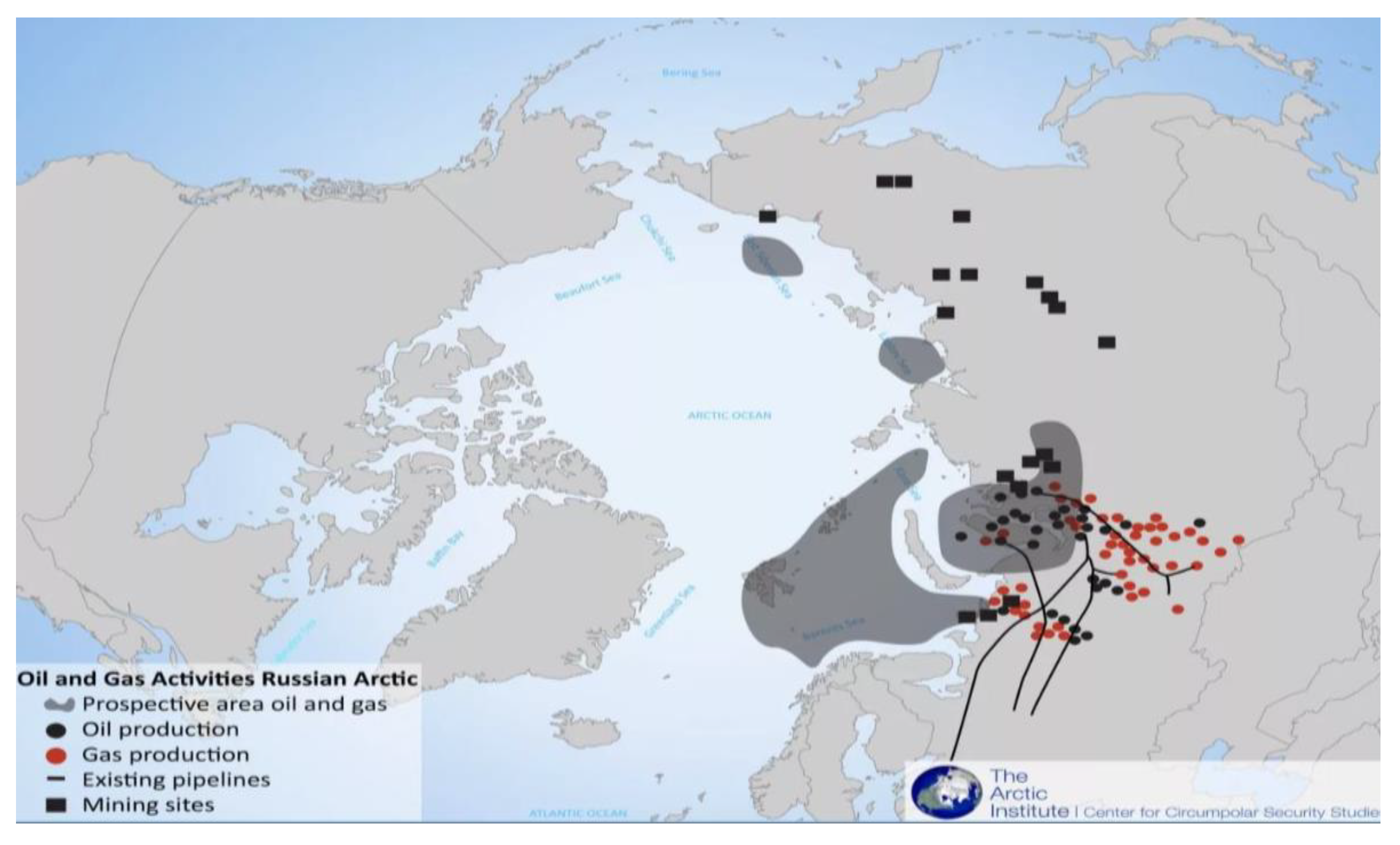
1. Introduction

Resource saving and the increasing requirements in environmental safety are a noticeable trend in the modern and world practice of transportation of hydrocarbons. Crude oil and oil product tankers emit Volatile Organic Compounds (VOCs) during the loading, transport, and discharging of their cargo. VOCs with a vapor pressure of more than 0.01 kPa at 239.15 K evaporate from the surface of crude oil in cargo tanks [1]. Approximately 2.4 million tons of VOCs, equivalent to about US$ 700 million, are lost each year during crude oil transport [2]. Volatile organic compounds emissions include propane (C₃H₈), butane (C₄H₁₀), pentane (C₅H₁₂), oxygen (O₂), carbon dioxide (CO₂), and small amounts of aromatic and sulfur-containing compounds. Under the influence of ultraviolet light and ozone, VOCs turn into dioxins [3]. Dioxins are environmental pollutants, and they are highly toxic to humans. VOCs also react with nitrogen oxides and form ozone when exposed to sunlight [4]. Ground-level ozone is one of the main components of urban smog [5]. The effects of ozone on a living organism are diverse. It causes morphological, biochemical, and functional changes in the body, significantly reducing its protective functions [6]. Besides, the opening of the mast riser on a tanker leads to significant losses of volatile hydrocarbons and an emergency shutdown of oil export due to an increase in the hydrocarbons concentration at the terminals above permissible values. For these reasons, it was decided to limit VOC emissions.

In 1997, the International Maritime organization created Annex VI of the MARPOL Convention, which entered into force in 2005. Annex VI describes measures to prevent air pollution, including VOCs, to provide terminals with facilities for receiving pollutants and state control. In addition, the Directive 2005/35/EC on pollution of ship sources and the imposition of fines for violations was adopted in the same year. Its goal was to tighten existing regulations to prevent the release of pollutants from ships. In particular, a protocol was adopted by a resolution of the Marine Environment Protection Committee, namely MEPC.176 (58), which entered into force on 1 July 2010 [7].

As global warming causes much of the area to melt, coastal countries have many opportunities [8]. The development of the Arctic coastline is especially important for the Russian Federation [9]. The Arctic route will shorten the route for ships by tendays compared to the Suez Canal. Cargo transportation statistics confirm this. In 2016, cargo traffic increased by more than 2.5 times compared to the previous year and amounted to 5.2 million tons. These facts indicate that the route is getting busier, and its usage is increasing exponentially [10]. The activities of the Russian Federation in the region can be traced in Figure 1.

The sale of energy resources through seaports is one of the main export priorities of most oil companies, Russia, Canada, the USA, and the Middle East. The volumes of oil exports through sea terminals are steadily increasing. For example, at the sea terminal, the final point of the Eastern Siberia-Pacific Ocean oil pipeline, oil exports in 2010 amounted to 15.3 million tons, and in 2016, 31.8 million tons. Owing to the increase in shipment volumes, the loss of hydrocarbons from evaporation also increases. Therefore, the trend towards increasing the transport of oil and oil products and the development of oil and gas fields in the Arctic zone pose a new challenge for humanity. It requires developing methods to prevent the negative impact on the Arctic environment, which is so sensitive to anthropogenic impacts.

There is a need to monitor the Arctic zone state and control activities that may harm it [11]. To do this, you need to predict and assess possible emissions and develop measures to prevent VOC emissions into the Arctic region atmosphere.

Countries possessing unequaled mineral potential have a unique chance to improve efficiency in this sector and extensive emerging opportunities to improve labor productivity in the industry [12]. Key preconditions for this are adopting and implementing organizational and legislative solutions in parallel with digital technology [13].

Estimated data on energy resource loss indicate that the Russian economy loses annually approximately 500 thousand tons of oil on the journey from extraction to the end-user in the absence of a vapor recovery unit on marine transport and during loading. The greatest losses occur in the fuel and energy industry itself [14]. The combination of various cost-effective technologies can increase project economic stability and financial attractiveness, which is one of the main conditions for further large-scale development [15,16,17,18].

This paper aims to offer possible estimation and forecasting of VOC emissions into the atmosphere when loading hydrocarbons into tankers.

This paper is organized as follows: Section 2 describes the proposed methods for estimating VOC emissions to the atmosphere; Section 3 presents investigations with corresponding calculations and graphs; Section 4 gives the results of the investigations, and Section 5 presents the conclusions of this article.

2. Methodology

2.1. Analytical Method for Estimating VOC Emissions into the Atmosphere

The amount of VOC emissions can be predicted analytically. A mathematical model is proposed that describes the dynamics of gas flows when loading tankers. The model determines the pressure growth curve in the gas space of tankers. This model can be used to estimate or prevent possible VOC emissions to the atmosphere. The nonlinear differential equation is based on the method of solving Runge–Kutta–Felberg differential equations. The model can be used in the design of new vapor recovery installations and the optimization of existing ones.

2.2. Experimental Method for Estimating VOC Emissions into the Atmosphere

An experimental method for estimating emissions is also proposed. Creating a laboratory stand for vapor recovery allows identifying VOC emissions’ actual values into the atmosphere when loading a tanker. This experimental apparatus has a purge air system. The use of a recuperator for the flow of working fluid after the expander and a pump at the expander’s outlet connected to a multiplier, which makes it possible to retain the amount of volatile organic compounds and convert them into gas.

We found that only a few studies have discussed the VRU by considering the type of crude oil. For instance, a few studies have confirmed crude oil processing as one of their major sources of VOCs, e.g., U.S. crude oil [19,20,21,22], Alaska crude oil, and Canadian crude oil [23,24,25]. However, it was impossible to provide any relationships between the type of crude oil from these data due to the different analytical methods and existing uncertainties. Therefore, it appears that there is a lack of comprehensive experimental research on VRU concerning various types of crude oils and operating conditions (temperature, humidity, etc.). Another factor is the lack of enough information related to the initial stages of crude oil production (before refineries), in which highly volatile compounds may escape into the atmosphere due to lack of appropriate measures.

3. Case Study

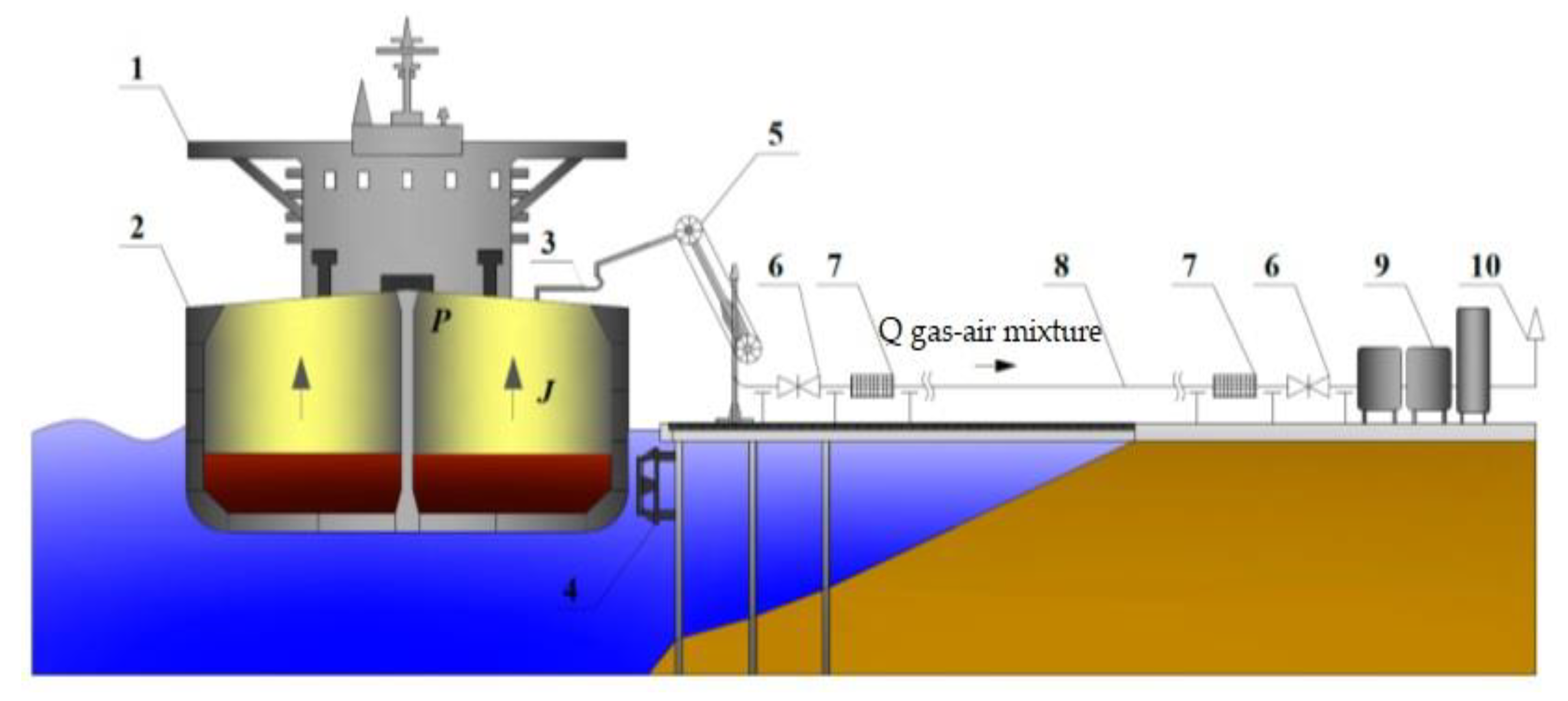
3.1. Conceptfor Constructing a Mathematical Model of the Gasspace Dynamics of a Tanker

In the process of filling the tanker, oil is supplied with a flow rate of Q_i. The volume of the tanker’s gas space changes, and the pressure inside the tanks P increases. The increase in pressure is caused not only by changes both in the volume of the gas space (GS) and by saturation of the GS with vapors of evaporating oil or petroleum product.

The movement of the gas-air mixture (GAM) with the flow of GAM occurs under the influence of the pressure drop between the tanker and the end point of the pipeline (pressure P_k), which removes the gas phase. In case the pressure exceeds the emergency value, the mast riser will open. GAM excess is diverted through the tanker’s ventilation system to the mast riser with a Q_mr flow rate. Figure 2 shows a diagram of the displacement of hydrocarbon vapors when loading a tanker.

To optimize the operation of VRU and correctly assess the loss of hydrocarbons through the mast riser, there is a need to describe the dynamics of gas flows when loading tankers.

The GS of a tanker equation in differential form is:

$$\frac{dP}{dt}·V+\frac{dV}{dt}·P=\frac{dG}{dt}·R·T,$$

(1)

P—the pressure in the gas space of the tanker, Pa; t—the time from the beginning of loading, s; V—the volume of the tanker’s gas space, m³; G—the mass of steam-and-gas in the gas space of the tanker, kg; R—the gas constant, J/kmol$·$K; T—the steam-and-gas temperature, K.

The current value of the volume of the GS of the tanker can be noted from Equation (1), where the change in volume over time is equal to the flow rate of the injection with the opposite sign ($\frac{\mathrm{dV}}{\mathrm{dt}}=-Q_i)$

$$\frac{dP}{dt}·\left(\frac{V_0-Q_i·t}{R·T}\right)+\left(-\frac{Q_i·t}{R·T}\right)·P=\frac{dG}{dt},$$

(2)

V₀—the initial volume of the tankers as space, m³; Q_i—volumetric flow rate of oil injection in the tanker, m³/h.

The change in the mass of the steam-and gas in the gas volume of the marine tanker in Equation (2) is defined as the difference between the mass entering the gas volume as a result of evaporation per unit time and the mass flow rate of the gas phase that is discharged through the pipeline to the vapor recovery units [16].

$$\frac{dG}{dt}=J·F-\frac{S\sqrt{P^2-P_k^2}}{\sqrt{R·T}\sqrt{2·ln\left(\frac{P}{P_k}\right)+\lambda \frac{L_{eff}}{D}}},$$

(3)

P_k—the pressure output in the pipeline of the gas phase, Pa; J—the intensity of mass transfer from the evaporation surface, kg/m²$·$s; F—the surface area of evaporation, m²; S—the line flow area of the gas phase, m²; L_eff—the effective length of the gas phase pipeline taking into all local resistances, m; D—the diameter of the gas phase pipeline, m; λ—the coefficient of hydraulic resistance, dimensionless.

The mathematical model is made with the following assumptions:

(1)

The inertance of the flow can be neglected due to the gas phase pipeline has a long length;

$$\lambda \frac{L_{eff}}{D}\gg 2·ln\left(\frac{P}{P_k}\right)$$

(4)

(2)

the gas constant is regarded as constant, R = const;

(3)

the law of mass transfer during evaporation is accepted exponentially.

The law of mass transfer during evaporation from the surface of the filling oil is adopted as.

$$J=J_b·e^{-\epsilon \tau },$$

(5)

$J_b$; $J_e$—flow density of evaporating oil respectively at the beginning and end of loading, kg/m²$·$s; $\epsilon$—the calculated coefficient equal to $ln\frac{J_e}{J_b}$, dimensionless; $\tau$—the loading time equal to the ratio of the current time elapsed from the beginning of loading time to the total tanker (0 ≤ $\tau$ ≤ 1), dimensionless.

Taking into account Equation (4), we obtain:

$$\frac{dP}{dt}·\left(\frac{V_0-Q_i·t}{R·T}\right)+\left(-\frac{Q_i}{R·T}\right)=J_b·F·e^{-\epsilon \tau }-\frac{P_k\sqrt{{\left(\frac{P}{P_k}\right)}^2-1}}{\frac{\sqrt{R·T}}{S}·\sqrt{\lambda ·\frac{L_{eff}}{D}}},$$

(6)

Divide both sides of Equation (6) by $\frac{Q_i·P_k}{R·T}$:

$$\frac{dP}{dt}·\left(\frac{V_{eff}-Q_i·t}{Q_i·P_k}\right)-\frac{P}{P_k}=\frac{J_b·F·R·T}{Q_i·P_k}·e^{-\epsilon \tau }-\frac{S\sqrt{R·T}}{Q_i·\sqrt{\lambda ·\frac{L_{eff}}{D}}}\sqrt{{\left(\frac{P}{P_k}\right)}^2-1}.$$

(7)

The following dimensionless groups are introduced:

$$\frac{P}{P_k}=y,$$

(8)

$$\frac{J_b·F·R·T}{Q_i·P_k}=\psi$$

(9)

$$\frac{Q_i·\sqrt{\lambda ·\frac{L_{Eff}}{D}}}{S\sqrt{R·T}}=\theta ,$$

(10)

$$\frac{t}{t_{end}}=\tau$$

(11)

Dimensionless groups have the following physical meaning:

y—the dimensionless pressure ratio, ψ—characterizes the contribution of evaporation to the overall dynamics of pressure growth in the gas space of the tanker, θ—characterizes the contribution of hydraulic resistances to the dynamics of pressure growth in the gas of the tanker, τ is the injection time.

Thus, we get the generalized differential equation in dimensionless parameters for studying the dynamics of pressure growth in the tanker’s gas space.

$$\frac{dy}{d\tau }·\left(1-\tau \right)=y+\psi ·e^{-\epsilon \tau }-\frac{\sqrt{y^2-1}}{\theta }.$$

(12)

This Equation (12) is a first-order nonlinear differential equation. The nonlinear differential equation and the algorithm are based on solving Runge–Kutta–Felberg differential equations of orders 4 and 5 (depending on the conditions of adaptation of the solution to its rate of change).

A calculation of the evaporation was carried out to study the influence of various factors on the dynamics of pressure changes in tankers’ gas space. The evaporation calculation was solved by Equation (3) for various values of the dimensionless parameters ψ and θ. Figure 3 shows a graph of changes in the dimensionless pressure drop for different values of the parameter ψ, for θ = 0.3 and ε = 0.8. Figure 4 shows a comparison of the results of modeling the dynamics of pressure changes in a tanker’s gas space with experimental data. This calculation shows a quantitative and qualitative determination of the dynamics of pressure growth in a tanke’s gas space.

The dimensionless parameter θ, which characterizes the system’s hydraulic resistance, has a significant impact on the dynamics of pressure growth in the gas space of a tanker.

The results obtained were compared with experimental data for more than 200 tankers. The suitability of the developed model was evaluated on the example of the SOPHIE SCHULTE tanker. The general view of the tanker is shown in Figure 5. The technical specifications are shown in

Table 1. Technical characteristics of the SOPHIE SCHULTE tanker.

Parameter	Value	Unit
Deadweight	115,583	tons
Dimensions	241 × 44	m
Method for inerting GS	exhaust gases	–
Pressure of saturated oil vapors on the raid	52.1	kPa

.

A comparison of simulation results with experimental data was performed.

Table 2. Comparing the results of modeling the dynamics of pressure changes in the tanker’s GP with experimental data.

№	The Current Time from Beginning of Loading, h	Experimental Data on Pressure in the Tanker’s GS, Pa	Pressure in the Tanker’s GS Calculated by Equation (12), Pa
1	0	101,815	101,815
2	0.41	102,595	105,124
3	1.08	104,365	105,612
4	1.41	109,215	107,570
5	2.08	110,645	109,866
6	2.41	112,355	110,511
7	2.58	112,455	110,761
8	3.41	111,035	111,443
9	3.91	111,225	111,580
10	4.41	110,835	111,602
11	5.41	110,445	111,468
12	6.41	110,395	111,236
13	7.41	110,345	110,982
14	8.41	110,495	110,730
15	9.41	110,235	110,487
16	10.41	110,495	110,253
17	10.91	110,385	110,139
18	11.41	107,005	106,389
19	11.91	108,325	106,309
20	12.91	106,075	104,007
21	13.33	101,325	101,325

shows a comparison of modeling the dynamics of pressure changes in the tanker’s GS with experimental data.

In addition, the results of modeling according to Equation (12) and experimental data on changes in the dynamics of pressure changes in the tanker’s GS are shown graphically in Figure 6.

From Figure 6, the developed model allows us to correctly determine the dynamics of pressure growth in the tanker’s gas space, both quantitatively and qualitatively. Some inconsistency of the model in changing injection modes with experimental data is explained by complex transitional processes, which can be accounted for using smoothing functions and there is some scientific interest for further work in this direction.

3.2. Laboratory Stand Concept for Vapor Recovery Unit

The sale of energy resources through seaports is one of the main export priorities of many oil companies [17]. This approach allows not only to diversify sales markets but also to avoid export quotas for transportation through the pipeline system. One of the vital problems is the loss of transported hydrocarbons. Because of this, enterprises incur ongoing costs for taxes for emissions of pollutants, lose valuable products, and cause huge damage to the environment [18]. In world practice, these problems are solved by the introduction of vapor recovery units (VRU). Several technologies are available to treat volatile organic compounds such as direct combustion, absorption, adsorption, membrane separation, compression, and condensation. Since VRUs cannot capture all VOCs, it is necessary to determine the effectiveness of installations experimentally before implementing them on terminals.

It is proposed to use a laboratory stand for VRUs to measure the actual values of VOCs emissions. The stand should contain vapor recovery technologies that are most suitable for the conditions of marine terminals that is, for large volumetric flow rate of loading oil or oil products in a tanker. The following technologies are suitable for this purpose:

−

adsorption;

−

absorption;

−

condensation.

The development of a laboratory stand will solve the existing problems by evaluating the effectiveness of vapor recovery technologies and VOC emissions. The experimental stand will allow us to determine a set of parameters of the VRUs and optimize their operation.

The stand will allow monitoring changes in the terminals’ state and the ability to control this process in the laboratory. This method allows predicting VOC emissions in the Arctic zone with the specified parameters.

Within the framework of this theory, a technological scheme for installing a laboratory stand was developed that is shown in Figure 7. Oil vapors are blown from tanks T1 and T2 through a detonation fire barrier, a drop breaker. Then they fall into the column of one of the technologies considered. The stand demonstrates the above-described vapor recovery technologies. After that, the undetected vapors are refined in a flow chromatography and bleed through a gas vent stack. The shut-off and control valves are controlled independently using a programmable logic controller (PLC). External modules connected to the PLC perform the role of collecting and converting information from all sensors. Then the data are processed and stored for further analysis.

4. Results

• The graphs of changes in dimensionless pressure for various parameters in Figure 5 and Figure 6 indicate that the most significant influence on the dynamics of pressure growth in the tanker’s gas space is exerted by the hydraulic resistance of the gas drainage system.
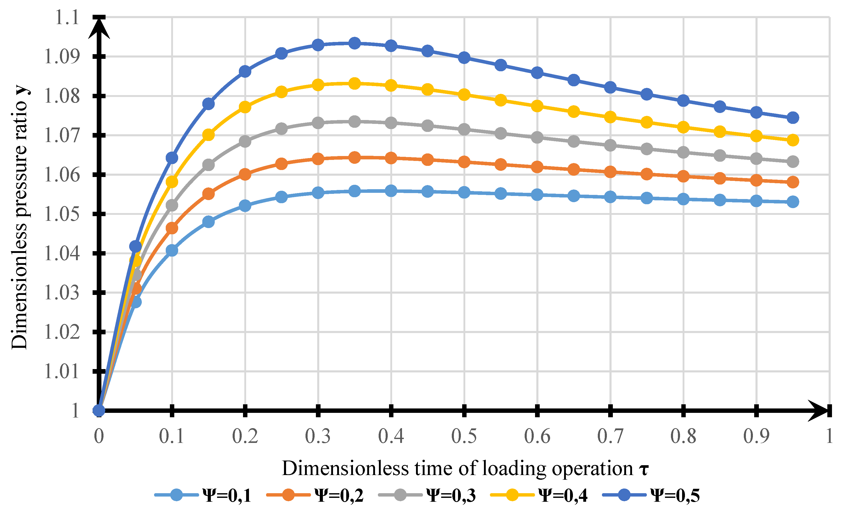
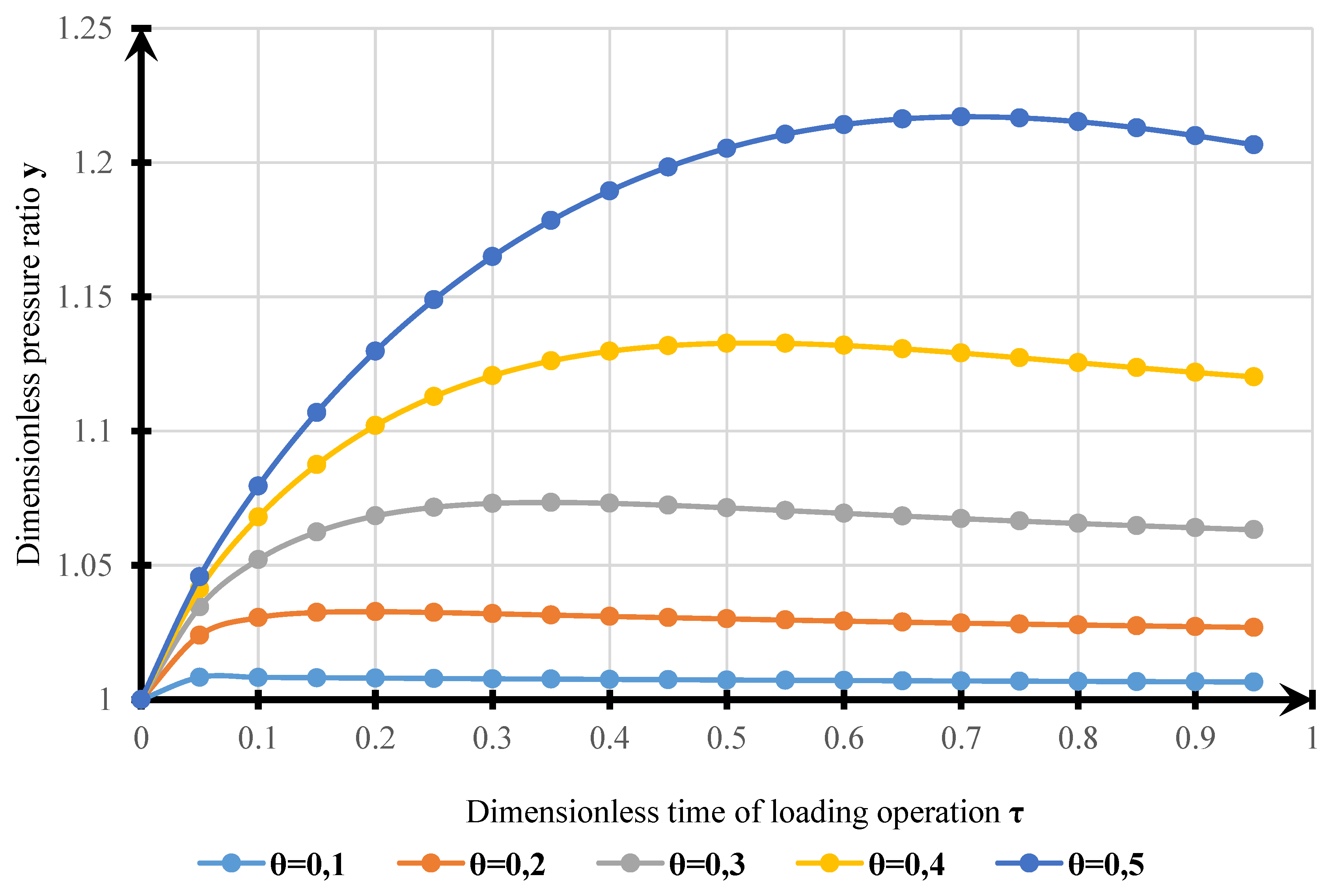
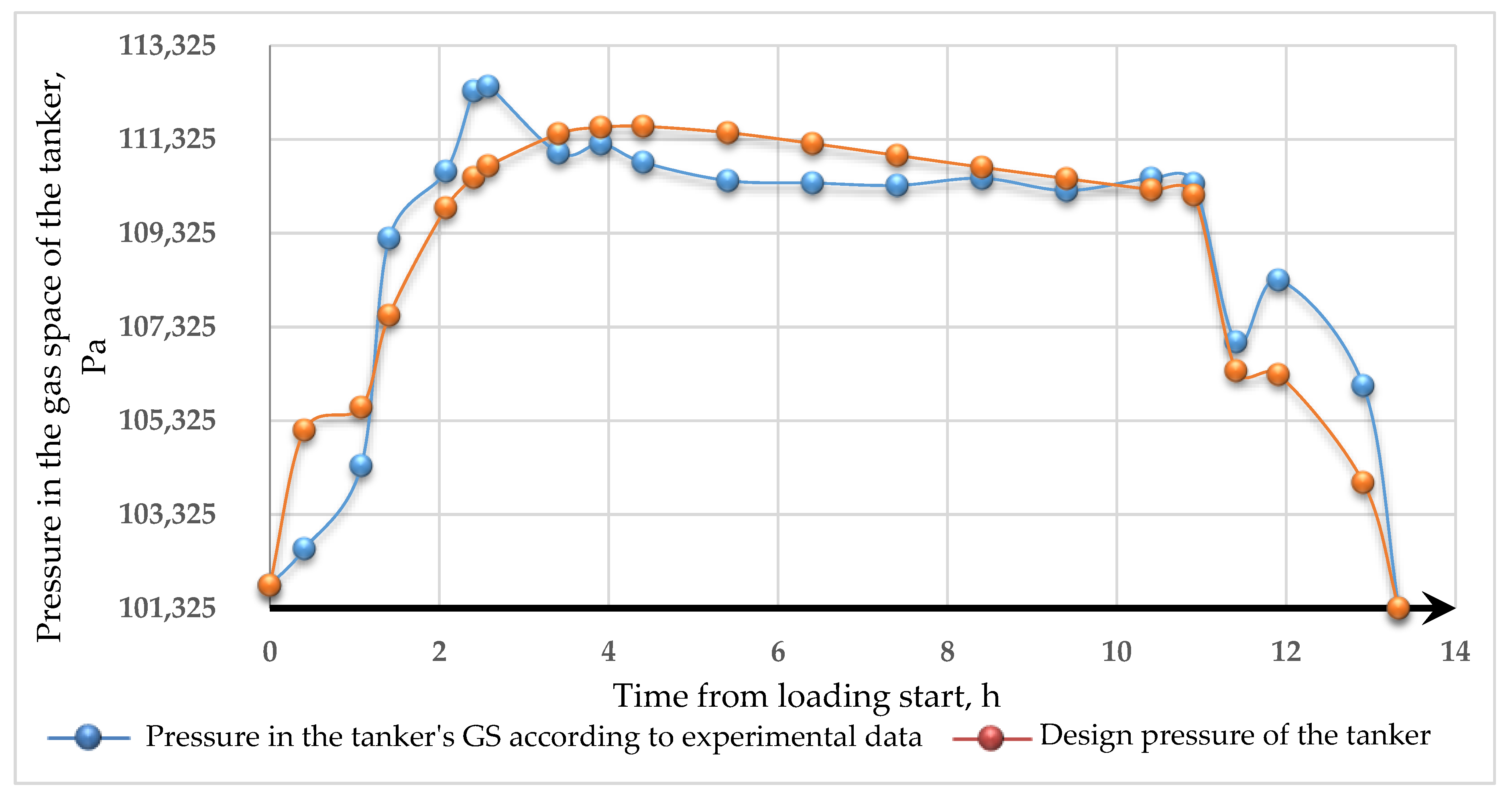
• The model obtained can be used for estimating VOC emissions when hydrocarbons are loaded into a tanker. The results of modeling the dynamics of pressure changes in the tanker’s GS with experimental data allowed us to determine the calculation error. The standard error of the model is 1215 Pa. Complex transitional processes explain the discrepancy of the model in changing the injection modes, and the account of re-existing processes can be made using smoothing functions.
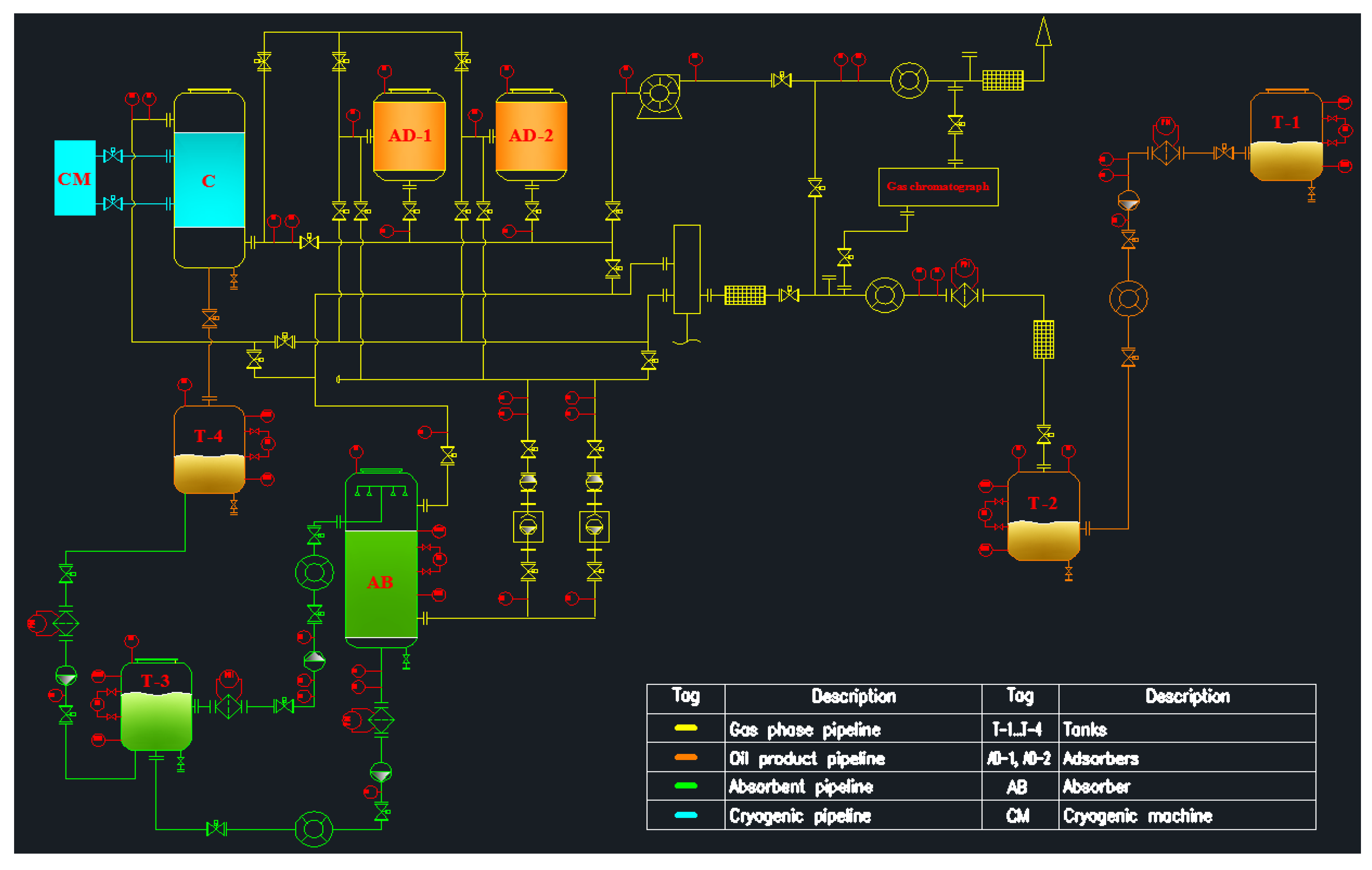
• An experimental method for estimating vapor emissions can be achieved by creating a stand in the laboratory, using the technological scheme developed in this work.

5. Conclusions

Regulation of VOCs emissions becomes mandatory, and the VOCs recovery system can provide solutions to the requirements for loading crude oil. Taking into account the world’s concern for sustainable development and the desire for environmental safety in oil transportation, especially in the Northern seas of the Arctic region, methods for estimating and preventing VOCs emissions were proposed, that are:

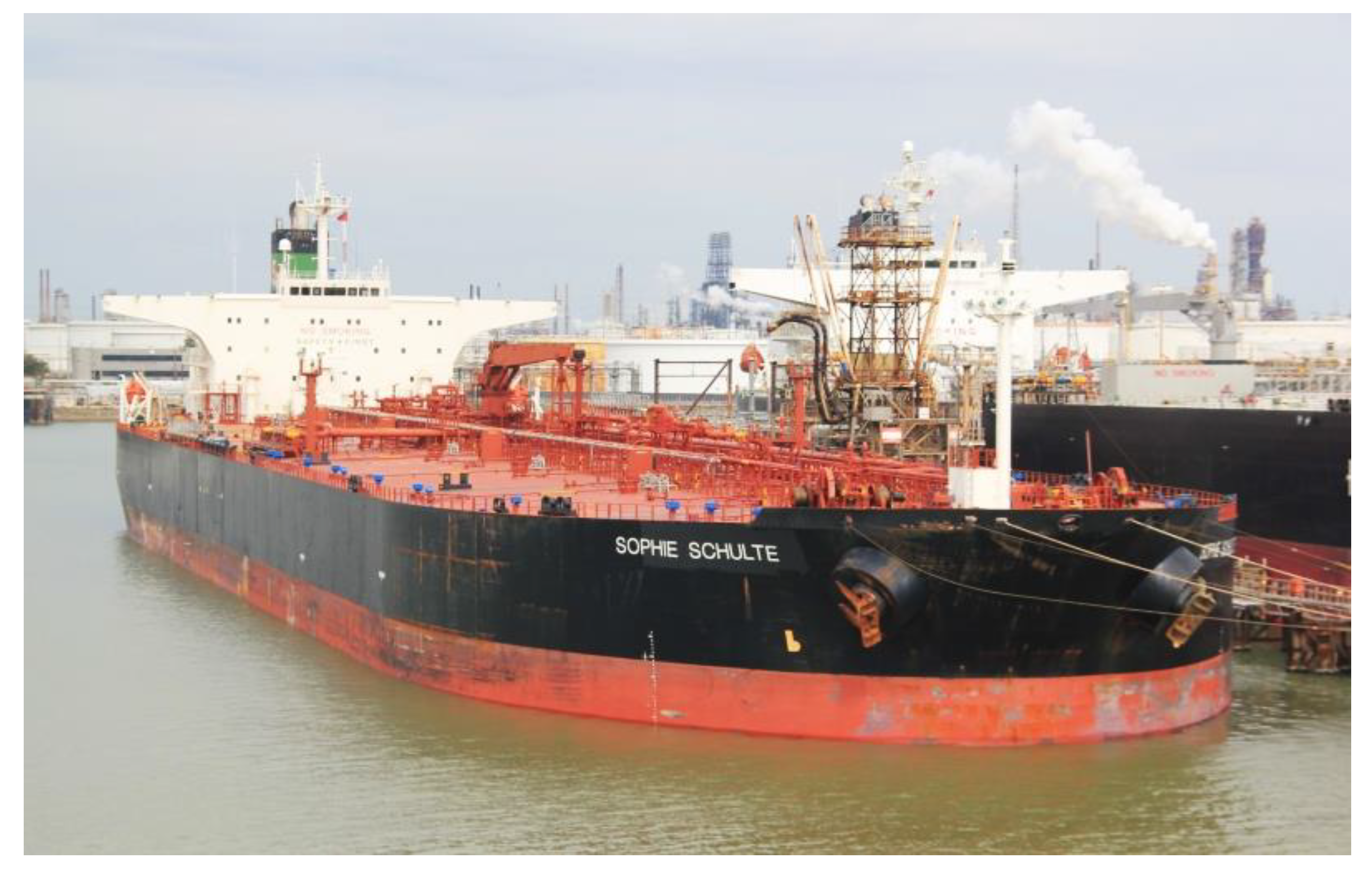
• A mathematical model was constructed that adequately describes the dynamics of gas flows during tanker loading. The results obtained were compared with the experimental data on the example of loading the SOPHIE SCHULTE tanker. Most of the error scans explain transitional processes when loading the tanker. Transitional processes are of some scientific interest for further work in this direction.
• The developed model can be used for estimating VOCs emissions. It also allows the evaluation of the capacity of existing pipeline systems for the removal of the gas phase and the design of new installations for the recovery of oil vapor. This would reduce emissions of VOCs and increase the security of the Arctic region’s ecosystem.
  It is also important to create a laboratory stand for an experimental method for estimating VOCs emissions and the effectiveness of the VRU.
• The technological scheme of a possible laboratory stand for vapor recovery was developed, which can evaluate the efficiency of the VRU of adsorption, absorption, and condensation technologies.

The obtained calculations of the experimental setup describe the dynamics of gas flows when loading a marine tanker. The results were compared with the experimental time using the example of an operating marine terminal.

The unique features of the conditions of the polar regions and, in particular, the Arctic region, such as an isolated location, impassable roads, extremely harsh climate, put forward very specific requirements for equipment, organization of operations, and training of personnel. Despite the high level of attention of oil companies to environmental safety, the problem of capturing oil vapor when loading tankers remain open to many existing and planned oil terminals. Therefore, humanity must continue to seek solutions to the problem of VOC pollution in the environment.

References

- The Council of the European Union. Council directive 1999/13/EC on the limitation of emissions of volatile organic compounds due to the use of organic solvents in certain activities and installations. Off. J. Eur. Commun. 1999, 4, 118–139. [Google Scholar]
- Buhaug, Ø.; Corbett, J.; Endresen, Ø.; Eyring, V.; Faber, J.; Hanayama, S. Second IMO GHG Study 2009; International Maritime Organization: London, UK, 2009. [Google Scholar]
- Spirig, C.; Neftel, A.; Ammann, C.; Dommen, J.; Grabmer, W.; Thielmann, A.; Schaub, A.; Beauchamp, J.D.; Wisthaler, A.; Hansel, A. Eddy covariance flux measurements of biogenic VOCs during ECHO 2003 using proton transfer reaction mass spectrometry. Atmos. Chem. Phys. 2005, 5, 465–481. [Google Scholar] [CrossRef]
- Bergin, M.S.; Russell, A.G.; Milford, J.B. Quantification of individual VOC reactivity using a chemically detailed, three-dimensional photochemical model. Environ. Sci. Technol. 1995, 29, 3029–3037. [Google Scholar] [CrossRef] [PubMed]
- Luecken, D.J.; Mebust, M.R. Technical challenges involved in implementation of VOC reactivity-based control of ozone. Environ. Sci. Technol. 2008, 42, 1615–1622. [Google Scholar] [CrossRef]
- Avery, R.J. Reactivity-based VOC control for solvent products: More efficient ozone reduction strategies. Environ. Sci. Technol. 2006, 40, 4845–4850. [Google Scholar] [CrossRef]
- Guidelines for the Development of a VOC Management Plan; IMO: London, UK, 2009.
- Tcvetkov, P.; Cherepovitsyn, A.; Fedoseev, S. The Changing Role of CO2 in the Transition to a Circular Economy: Review of Carbon Sequestration Projects. Sustainability 2019, 11, 5834. [Google Scholar] [CrossRef]
- Litvinenko, V. Russian developments of equipment and technology of deep hole drilling in ice. In Innovation-Based Development of the Mineral Resources Sector: Challenges and Prospects, Proceedings of the 11th Russian-German Raw Materials Conference, Potsdam, Germany, 7–8 November 2018; Taylor & Francis Group: London, UK, 2018. [Google Scholar]
- Ilinova, A.; Cherepovitsyn, A.; Evseeva, O. Stakeholder Management: An Approach in CCS Projects. Resources 2018, 7, 83. [Google Scholar] [CrossRef]
- Mariya, A.P.; Alexey, V.A. Reutilization Prospects of Diamond Clay Tailings at the Lomonosov Mine. Northwest. Russ. Miner. 2020, 10, 517. [Google Scholar] [CrossRef]
- Litvinenko, V.S. Digital Economy as a Factor in the Technological Development of the Mineral Sector. Nat. Resour. Res. 2020, 29, 1521–1541. [Google Scholar] [CrossRef]
- Pashkevich, M.A.; Petrova, T.A. Recyclability of ore beneficiation wastes at the Lomonosov Deposit. J. Ecol. Eng. 2019, 20, 27–33. [Google Scholar] [CrossRef]
- Abramovich, B.; Sychev, Y. Problems of ensuring energy security for enterprises from the mineral resources sector. J. Min. Inst. 2016, 217, 132–139. [Google Scholar]
- Romasheva, N.V.; Kruk, M.N.; Cherepovitsyn, A.E. Propagation perspectives of CO2 sequestration in the world. Int. J. Mech. Eng. Technol. 2018, 9, 1877–1885. [Google Scholar]
- Yang, G.; Zhai, X.Q. Optimal design and performance analysis of solar hybrid CCHP system considering influence of building type and climate condition. Energy 2019, 174, 647–663. [Google Scholar] [CrossRef]
- Tcvetkov, P.; Cherepovitsyn, A.; Makhovikov, A. Economic assessment of heat and power generation from small-scale liquefied natural gas in Russia. Energy Rep. 2020, 6, 391–402. [Google Scholar] [CrossRef]
- Mulder, T. VOC recovery systems. Hydrocarb. Eng. 2007, 12, 37–40. [Google Scholar]
- Gilman, J.B.; Lerner, B.M.; Kuster, W.C.; De Gouw, J.A. Source signature of volatile organic compounds from oil and natural gas operations in northeastern Colorado. Environ. Sci. Technol. 2013, 47, 1297–1305. [Google Scholar] [CrossRef]
- Helmig, D.; Thompson, C.R.; Evans, J.; Boylan, P.; Hueber, J.; Park, J.H. Highly elevated atmospheric levels of volatile organic compounds in the Uintah Basin, Utah. Environ. Sci. Technol. 2014, 48, 4707–4715. [Google Scholar] [CrossRef]
- Koss, A.; Yuan, B.; Warneke, C.; Gilman, J.B.; Lerner, B.M.; Veres, P.R.; Thompson, C.R. Observations of VOC emissions and photochemical products over US oil-and gas-producing regions using high-resolution H3O+ CIMS (PTR-ToF-MS). Atmos. Meas. Tech. 2017, 10, 2941. [Google Scholar] [CrossRef]
- Warneke, C.; Geiger, F.; Edwards, P.M.; Dube, W.; Pétron, G.; Kofler, J.; Lerner, B. Volatile organic compound emissions from the oil and natural gas industry in the Uinta Basin, Utah: Point sources compared to ambient air composition. Atmos. Chem. Phys. Discuss. 2014, 14, 11895–11927. [Google Scholar] [CrossRef]
- Hanna, S.R.; Drivas, P.J. Modeling VOC emissions and air concentrations from the Exxon Valdez oil spill. Air Waste 1993, 43, 298–309. [Google Scholar] [CrossRef]
- Simpson, I.J.; Blake, N.J.; Barletta, B.; Diskin, G.S.; Fuelberg, H.E.; Gorham, K.; Weinheimer, A.J. Characterization of trace gases measured over Alberta oil sands mining operations: 76 speciated C2-C10 volatile organic compounds (VOCs), CO2, CH4, CO, NO, NO2, NOy, O3 and SO2. Atmos. Chem. Phys. 2010, 10, 11931–11954. [Google Scholar] [CrossRef]
- Yang, C.; Wang, Z.; Li, K.; Hollebone, B.P.; Brown, C.E.; Landriault, M. Determination of Volatile Organic Compounds over Crude Oils Using Novel Automatic Liquid Sampler-Headspace (ALS-HS) Gas Chromatography/Mass Spectrometry. In Proceedings of the Thirtieth AMOP Technical Seminar, Environment Canada, Ottawa, ON, Canada, 5–7 June 2007; pp. 49–59. [Google Scholar]