Improvement of Marine Steam Turbine Conventional Exergy Analysis by Neural Network Application


Abstract
1. Introduction
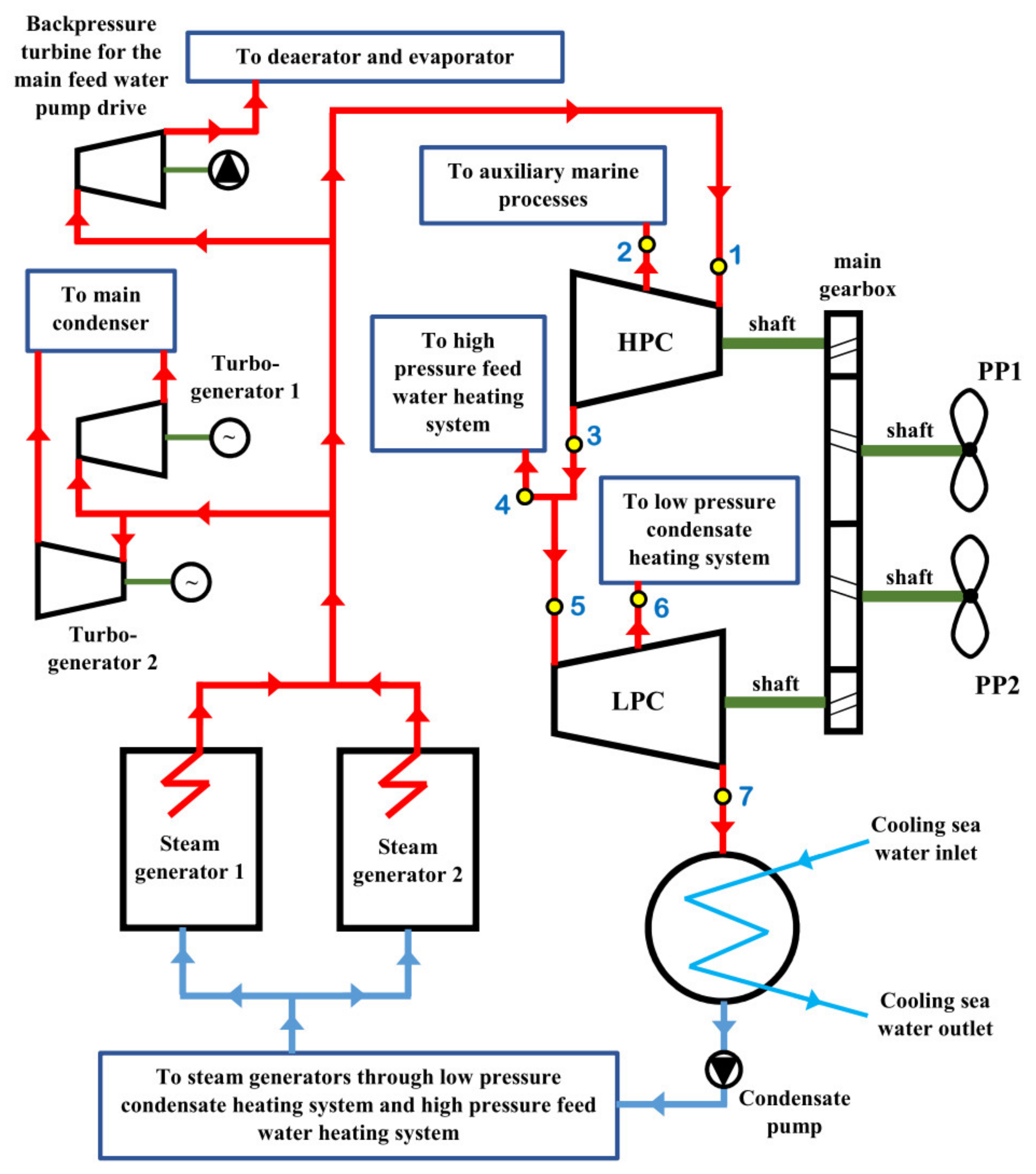
2. Description and Operation Principle of the Analyzed Main Marine Steam Turbine
3. Conventional Exergy Analysis of Main Marine Steam Turbine and Each of its Cylinders
3.1. Overall Exergy Analysis Balances and Equations
3.2. Equations for the Exergy Aanalysis of Main Marine Steam Turbine and Its Cylinders
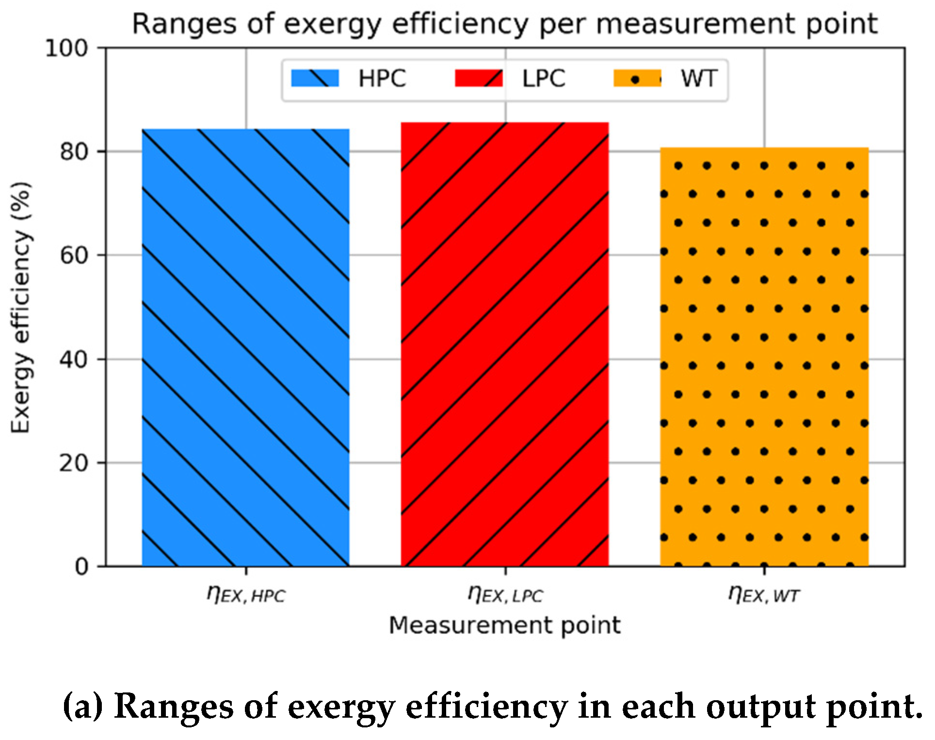
3.2.1. High Pressure Cylinder (HPC)
3.2.2. Low Pressure Cylinder (LPC)
3.2.3. Whole Turbine (WT)
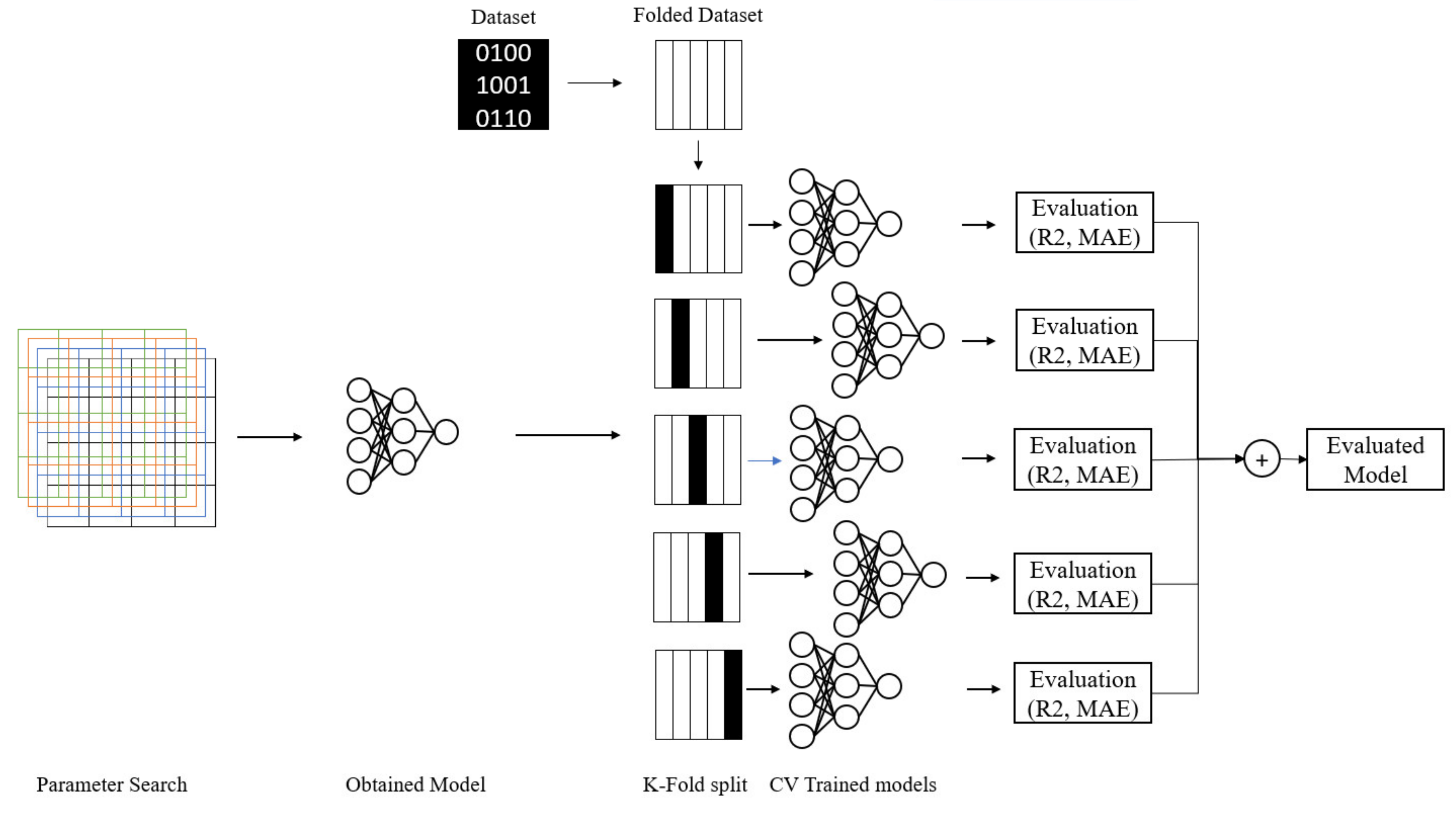
4. Exergy Analysis of Main Marine Steam Turbine and Each of its Cylinders by MLP Neural Network Application
- Eliminate the unwanted values such as Rectified linear unit—ReLU ()—used to eliminate negative values [95],
- Map the input files to a certain range such as sigmoid (logistic) function which maps the values to a range of ] () or hyperbolic tangent function which maps them to the range of [−1, 1] (),
5. Steam Operating Parameters Required for the Exergy Analysis
5.1. Conventional Exergy Analysis
5.2. Exergy Analysis by MLP Neural Network Application
- (1)
- By using all collected data, developed mechanical power, exergy destruction and exergy efficiency of each cylinder are calculated as well as the whole turbine at each of the 24 loads with the conventional exergy analysis.
- (2)
- Results obtained by conventional exergy analysis are then used for MLP training and testing.
- (3)
- MLP is trained for every hyperparameter combination given in Table 5, which results in a total of 442,368 models when the aforementioned cross-validation process is applied.
- (4)
- The results of 442,368 models are compared across 72 input/output parameter combinations, given in Table 5, in order to determine the best possible model architecture for each of the aforementioned combinations.
5.3. Measuring Equipment
6. Results and Discussion
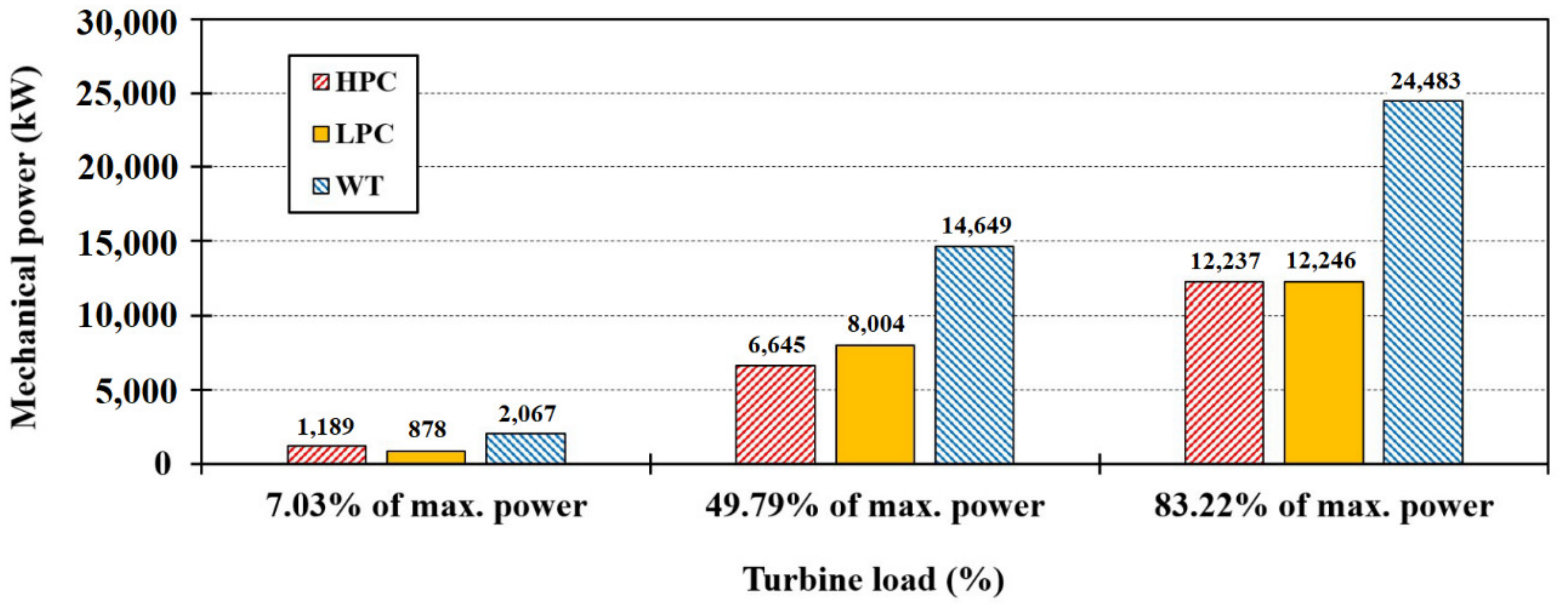
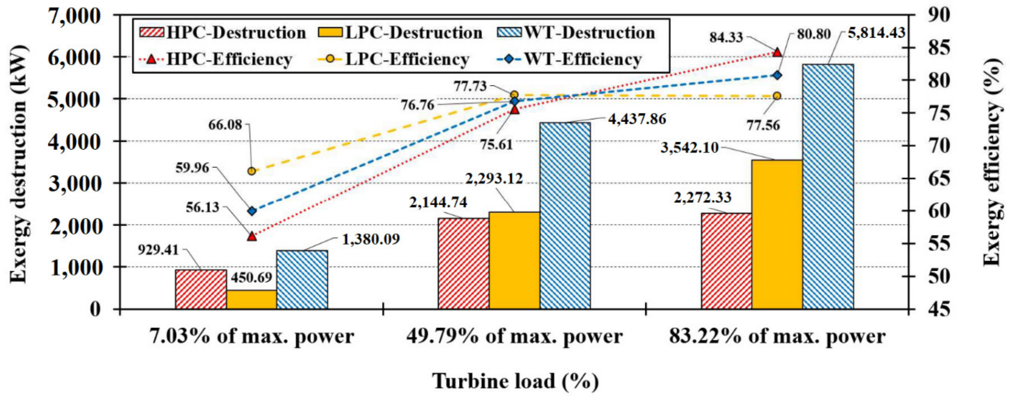
6.1. The Results of the Conventional Exergy Analysis
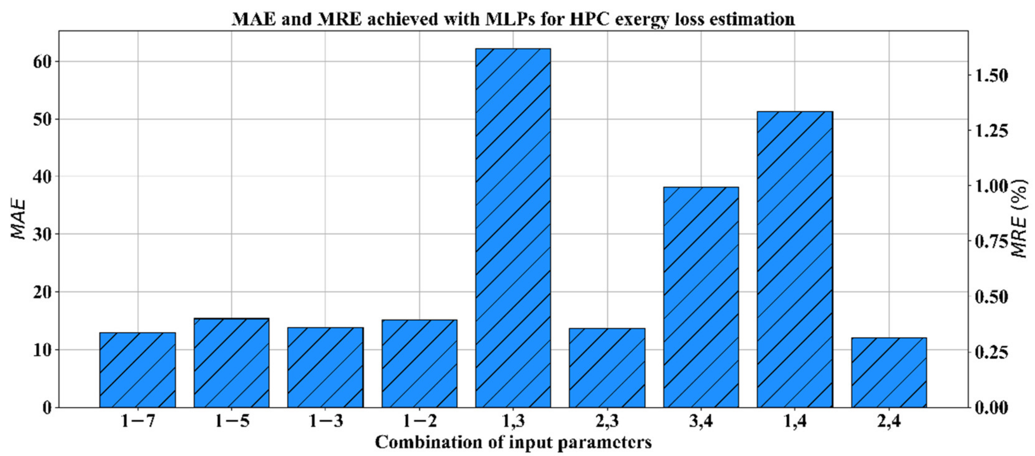
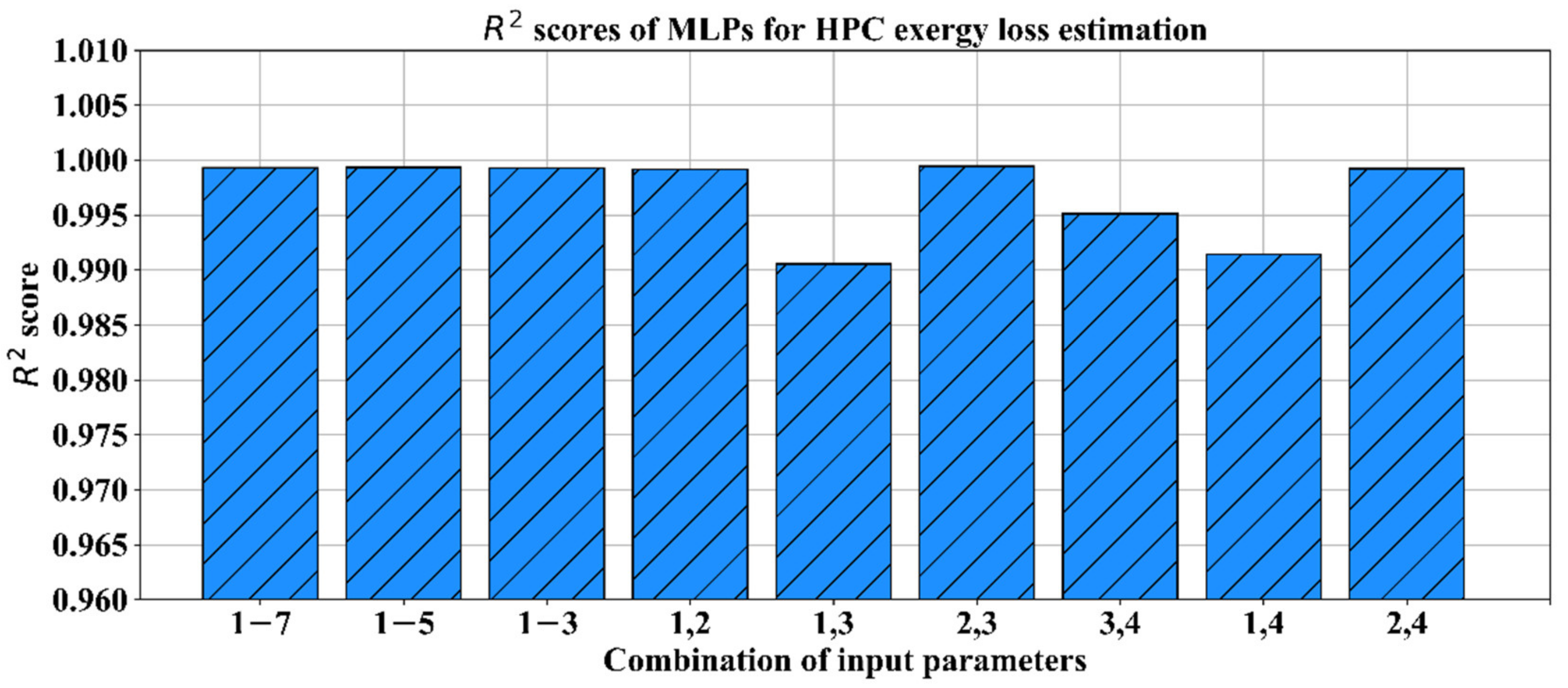
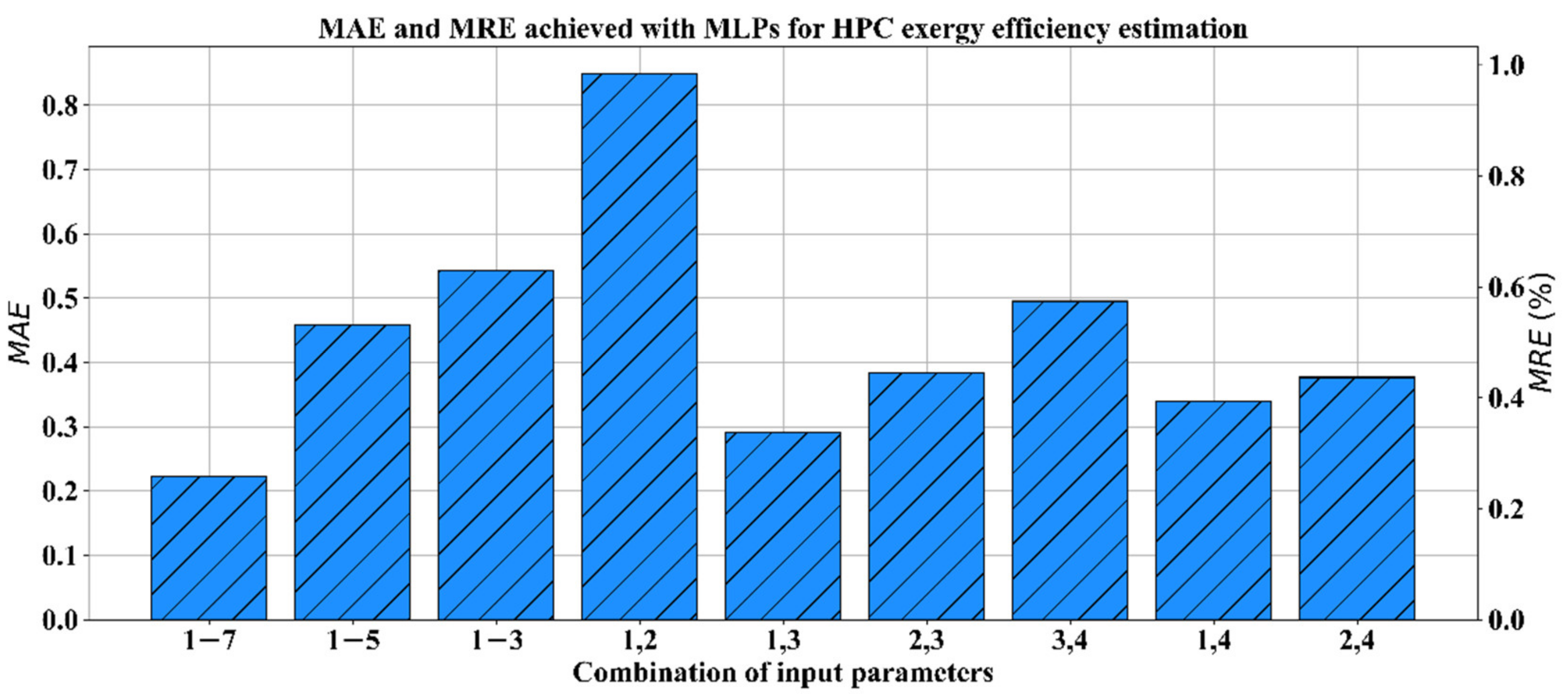
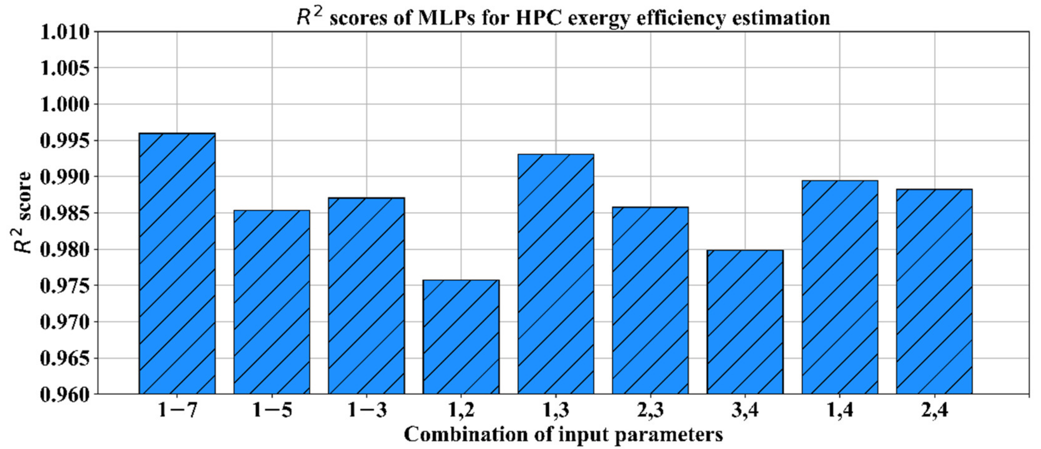
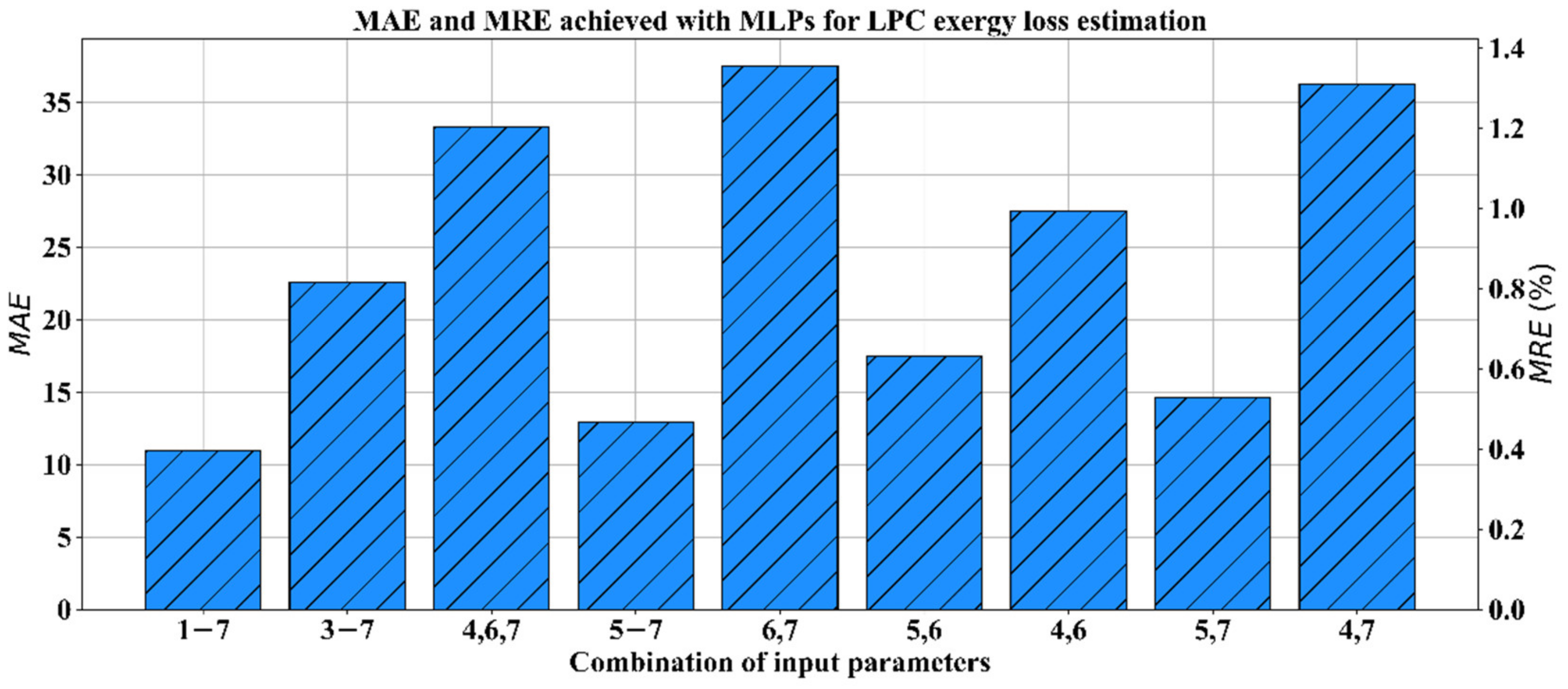
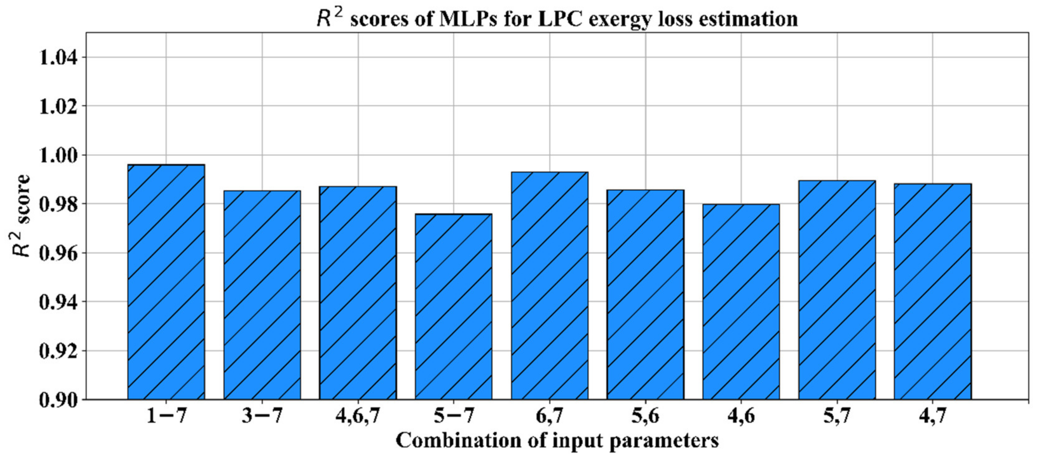
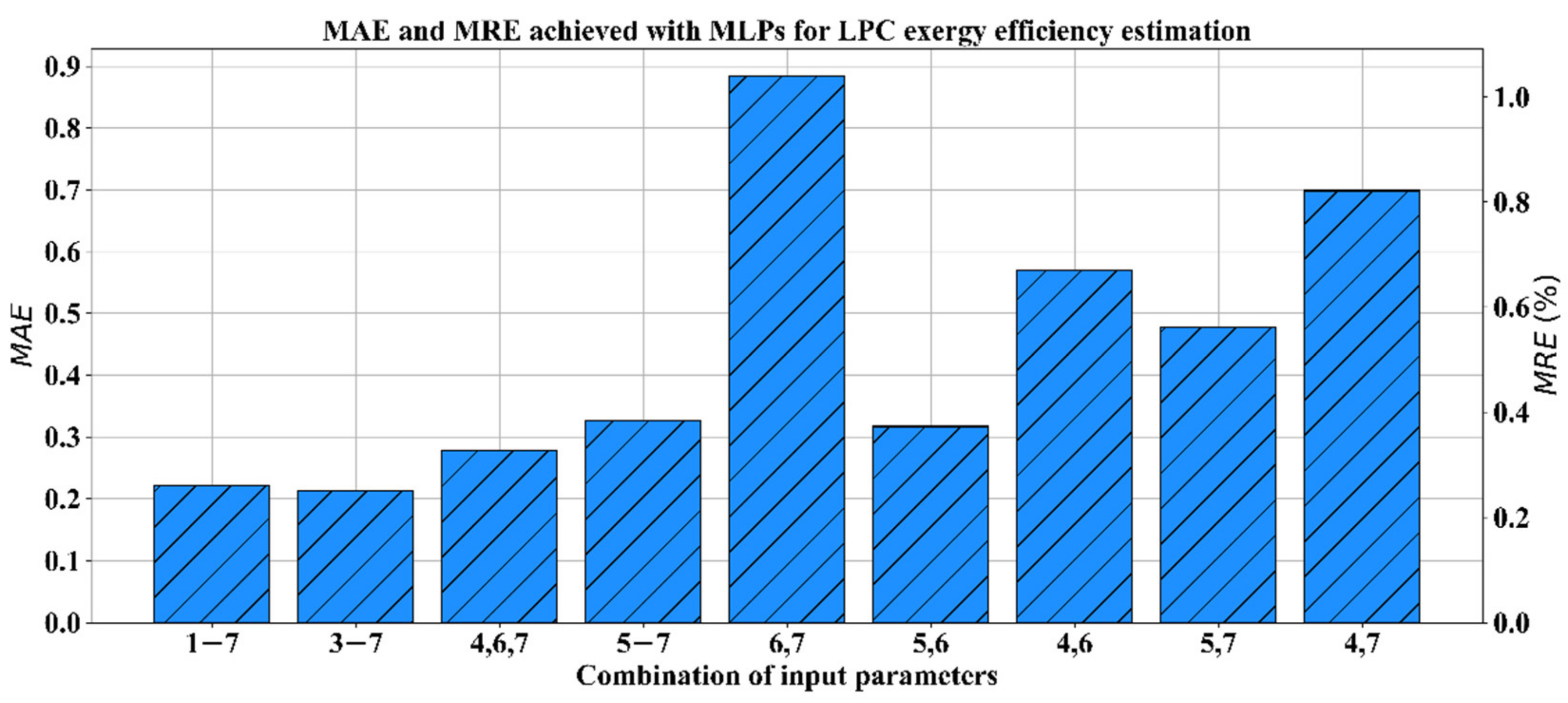
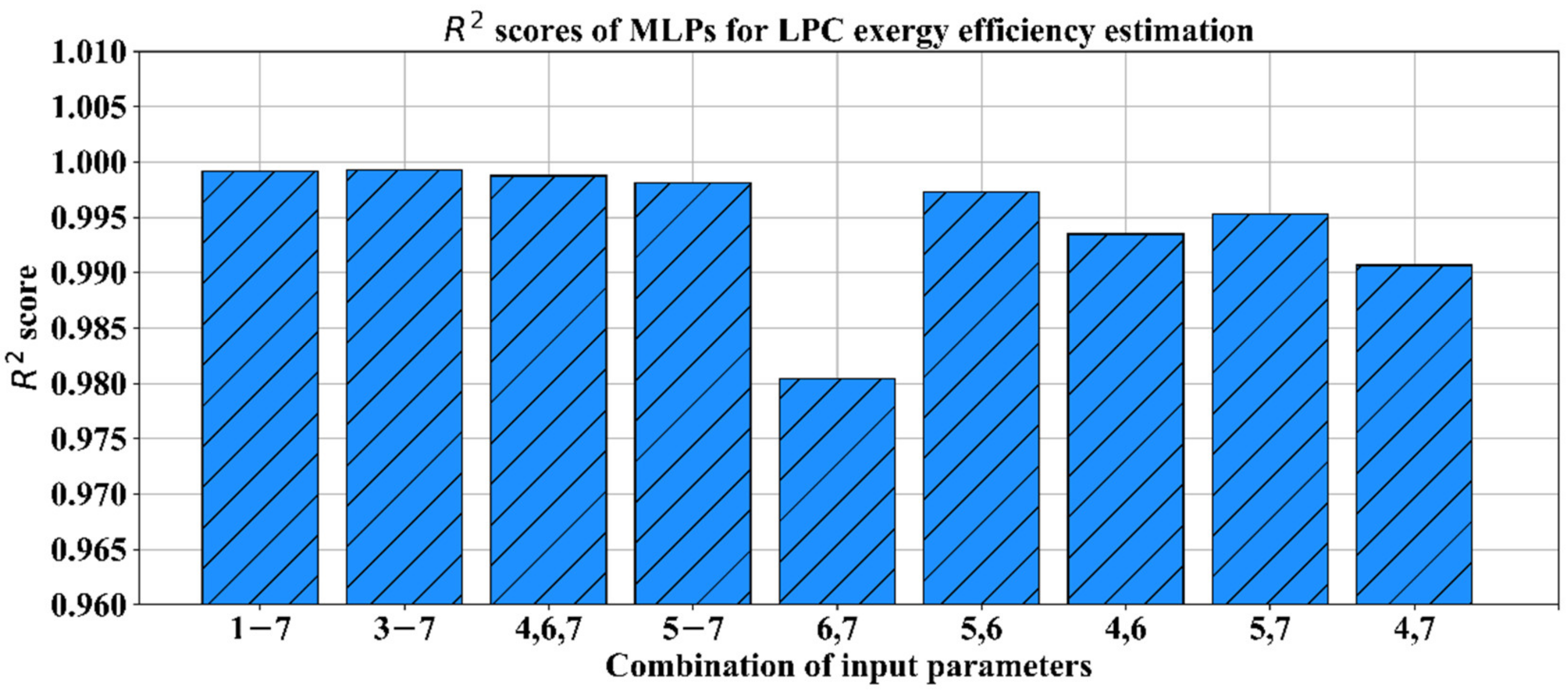
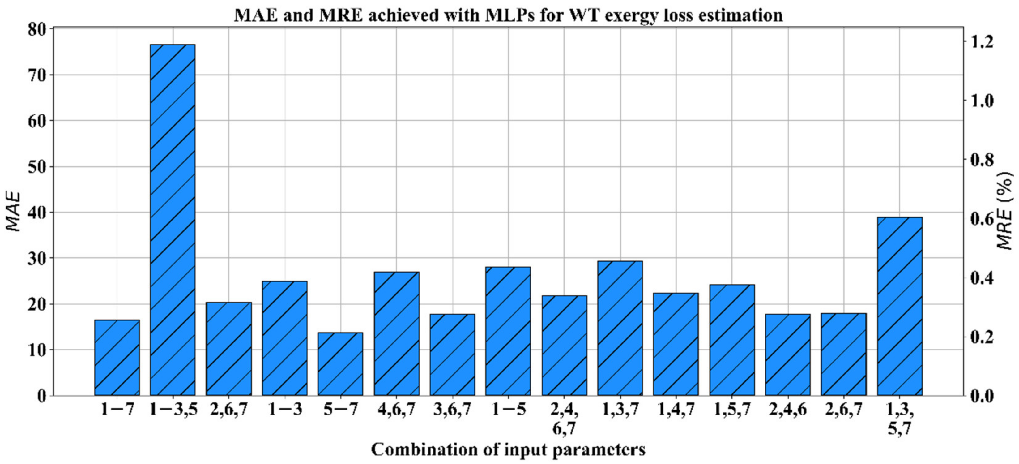
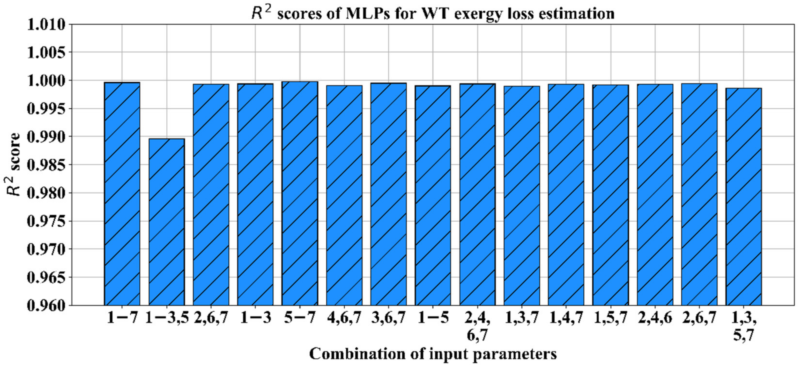
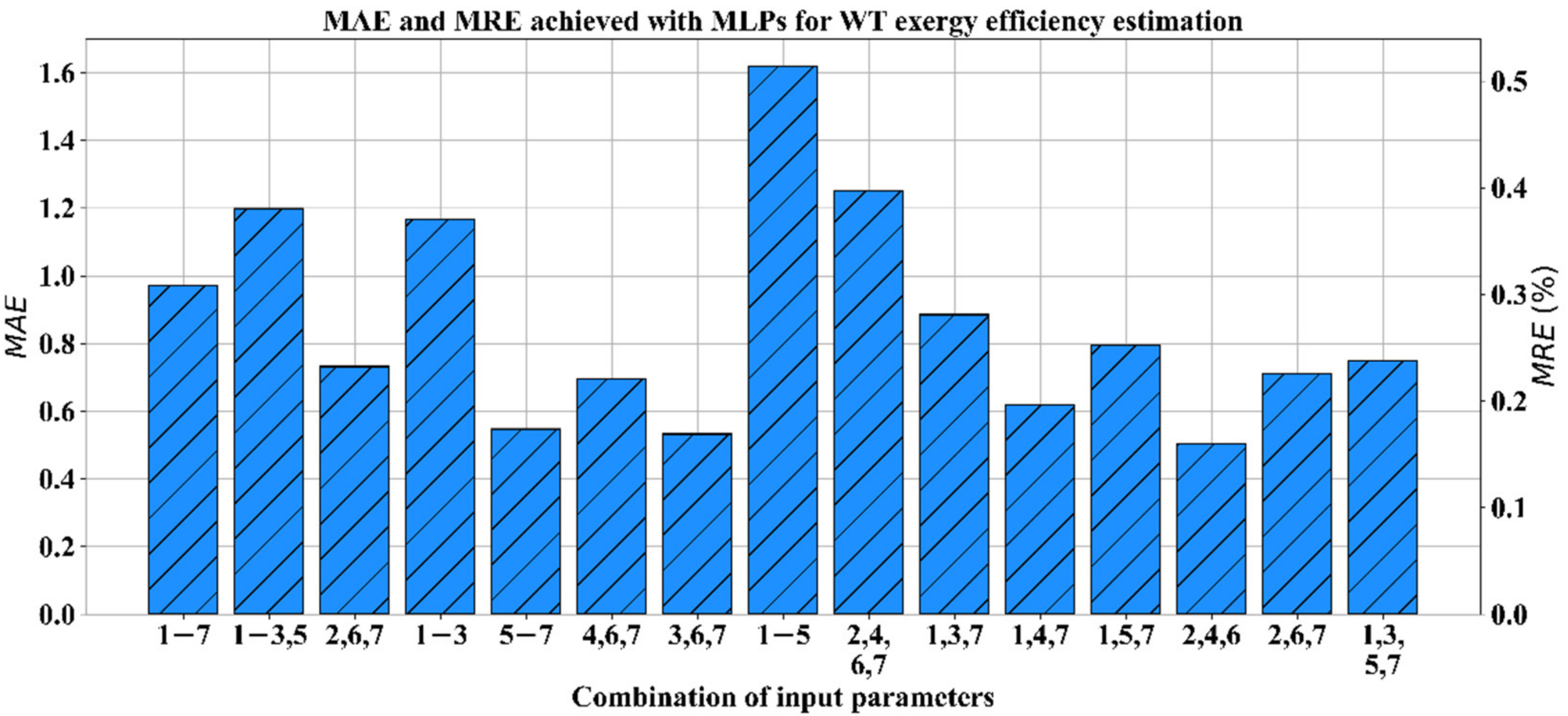
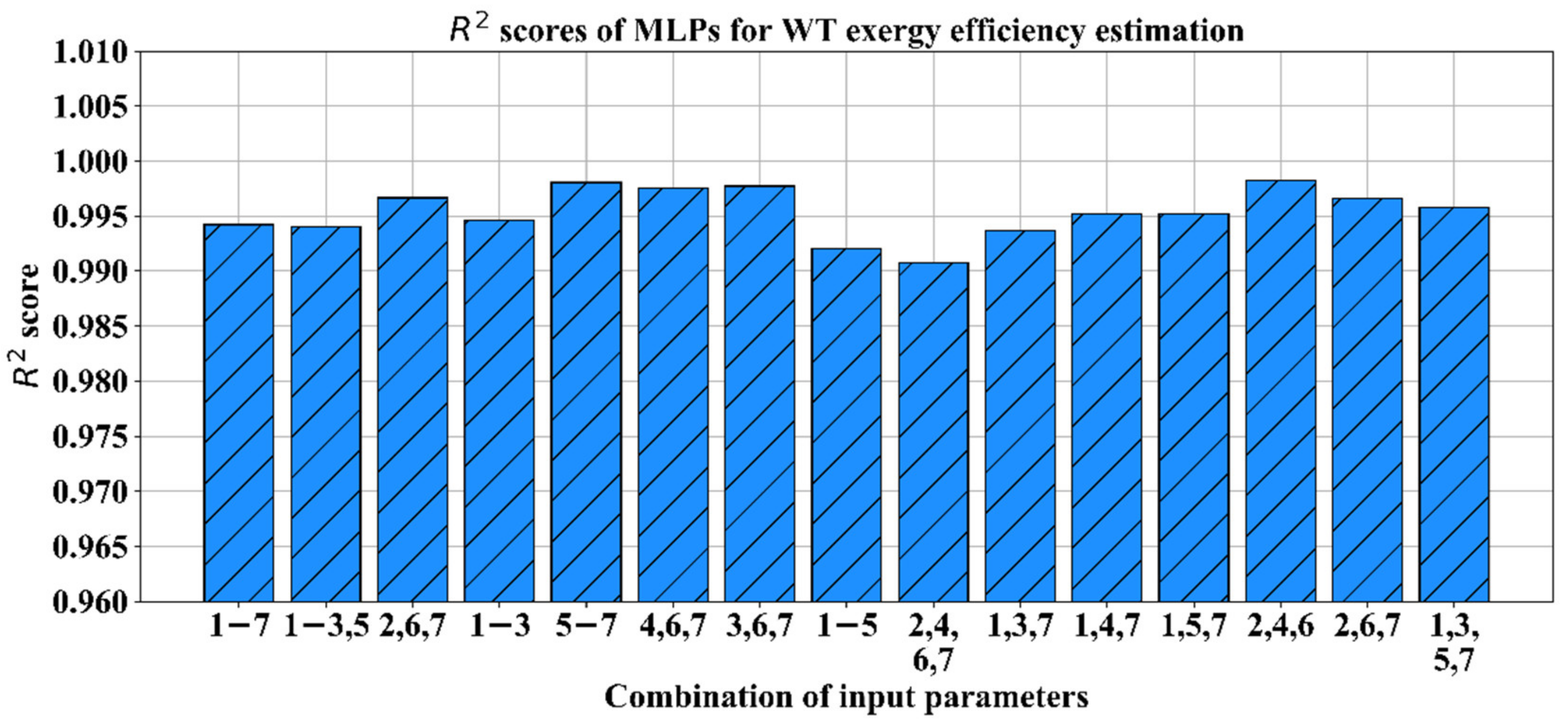
6.2. Exergy Analysis Results by MLP Neural Network Application
7. Conclusions
- (1)
- To determine optimal turbine operating points for the measurement of steam temperature, pressure and mass flow rate. The goal will be to find three or four operating points of which the measurement results, along with MLP application, can be used for exergy analysis parameters prediction of the whole turbine and each cylinder at any load, with the lowest possible errors.
- (2)
- Extensive measurements during a long time period will allow determining performance degradation coefficients for the whole analyzed turbine and each of its cylinders. Implementation of such coefficients inside MPL structure will allow accurate and precise predicting of turbine exergy analysis parameters for the entire period of its operation.
- (3)
- Investigate if the same technique can be applied for other main marine steam turbines (especially for newer variants, which consist of three cylinders and steam reheating).
Author Contributions
Funding
Conflicts of Interest
Appendix A. Specification of Used Measuring Equipment

| → Greisinger GTF 601-Pt100 | |
|---|---|
| Measuring range: | −200 to +600 °C |
| Response time: | approximate 10 s |
| Standard: | 1/3 DIN class B |
| Error ranges: | |
| → Greisinger GTF 401-Pt100 | |
| Measuring range: | −50 to +400 °C |
| Response time: | approximate 10 s |
| Standard: | DIN class B |
| Error ranges: | |
| → Yamatake JTG960A | |
|---|---|
| Measuring span: | 0.7 to 14 MPa |
| Setting range: | −0.1 to 14 MPa |
| Working pressure range: | 2.0 kPa to 14 MPa |
| Accuracy: | |
| → Yamatake JTG940A | |
| Measuring span: | 35 to 3500 kPa |
| Setting range: | −100 to 3500 kPa |
| Working pressure range: | 2.0 kPa to 3500 kPa |
| Accuracy: | |
| → Yamatake JTD960A | |
|---|---|
| Measuring span: | 0.25 to 14 MPa |
| Setting span: | −100 to 14 MPa |
| Working pressure range: | 2.0 kPa to 14 MPa |
| Accuracy: | |
| → Yamatake JTD930A | |
| Measuring span: | 35 to 700 kPa |
| Setting span: | −100 to 700 kPa |
| Working pressure range: | 2.0 kPa to 14 MPa |
| Accuracy: | |
| → Yamatake JTD920A | |
| Measuring span: | 0.75 to 100 kPa |
| Setting span: | −100 to 100 kPa |
| Working pressure range: | 2.0 kPa to 14 MPa |
| Accuracy: | |
| → Yamatake JTD910A | |
| Measuring span: | 0.1 to 2 kPa |
| Setting span: | −1 to 1 kPa |
| Working pressure range: | up to 210 kPa |
| Accuracy: | |
References
- Tontu, M.; Sahin, B.; Bilgili, M. An exergoeconomic–environmental analysis of an organic Rankine cycle system integrated with a 660 MW steam power plant in terms of waste heat power generation. Energy Sources Part A Recovery Util. Environ. Eff. 2020, 2020, 1–22. [Google Scholar] [CrossRef]
- Elhelw, M.; Al Dahma, K.S. Utilizing exergy analysis in studying the performance of steam power plant at two different operation mode. Appl. Therm. Eng. 2019, 150, 285–293. [Google Scholar] [CrossRef]
- Uysal, C.; Kurt, H.; Kwak, H.Y. Exergetic and thermoeconomic analyses of a coal-fired power plant. Int. J. Ther. Sci. 2017, 117, 106–120. [Google Scholar] [CrossRef]
- Naserbegi, A.; Aghaie, M.; Minuchehr, A.; Alahyarizadeh, G. A novel exergy optimization of Bushehr nuclear power plant by gravitational search algorithm (GSA). Energy 2018, 148, 373–385. [Google Scholar] [CrossRef]
- Wilding, P.R.; Murray, N.R.; Memmott, M.J. The use of multi-objective optimization to improve the design process of nuclear power plant systems. Ann. Nucl. Energy 2020, 137, 107079. [Google Scholar] [CrossRef]
- Adibhatla, S.; Kaushik, S.C. Exergy and thermoeconomic analyses of 500 MWe sub critical thermal power plant with solar aided feed water heating. Appl. Therm. Eng. 2017, 123, 340–352. [Google Scholar] [CrossRef]
- Mehrpooya, M.; Ghorbani, B.; Sadeghzadeh, M. Hybrid solar parabolic dish power plant and high-temperature phase change material energy storage system. Int. J. Energy Res. 2019, 43, 5405–5420. [Google Scholar] [CrossRef]
- Idris, M.N.M.; Hashim, H.; Razak, N.H. Spatial optimisation of oil palm biomass co-firing for emissions reduction in coal-fired power plant. J. Clean. Prod. 2018, 172, 3428–3447. [Google Scholar] [CrossRef]
- Kim, D.; Kim, K.T.; Park, Y.K. A Comparative Study on the Reduction Effect in Greenhouse Gas Emissions between the Combined Heat and Power Plant and Boiler. Sustainability 2020, 12, 5144. [Google Scholar] [CrossRef]
- Li, X.; Teng, Y.; Zhang, K.; Peng, H.; Cheng, F.; Yoshikawa, K. Mercury Migration Behavior from Flue Gas to Fly Ashes in a Commercial Coal-Fired CFB Power Plant. Energies 2020, 13, 1040. [Google Scholar] [CrossRef]
- Nazir, S.M.; Bolland, O.; Amini, S. Analysis of combined cycle power plants with chemical looping reforming of natural gas and pre-combustion CO2 capture. Energies 2018, 11, 147. [Google Scholar] [CrossRef]
- Javadi, M.A.; Hoseinzadeh, S.; Ghasemiasl, R.; Heyns, P.S.; Chamkha, A.J. Sensitivity analysis of combined cycle parameters on exergy, economic, and environmental of a power plant. J. Ther. Anal. Calor. 2020, 139, 519–525. [Google Scholar] [CrossRef]
- Rao, A.G.; Van den Oudenalder, F.S.C.; Klein, S.A. Natural gas displacement by wind curtailment utilization in combined-cycle power plants. Energy 2019, 168, 477–491. [Google Scholar] [CrossRef]
- Kotowicz, J.; Brzęczek, M. Analysis of increasing efficiency of modern combined cycle power plant: A case study. Energy 2018, 153, 90–99. [Google Scholar] [CrossRef]
- Pattanayak, L.; Sahu, J.N.; Mohanty, P. Combined cycle power plant performance evaluation using exergy and energy analysis. Env. Progr. Sust. Energy 2017, 36, 1180–1186. [Google Scholar] [CrossRef]
- Okubo, M.; Kuwahara, T. New Technologies for Emission Control in Marine Diesel Engines; Butterworth-Heinemann: Oxford, UK, 2020. [Google Scholar]
- Sartomo, A.; Santoso, B.; Muraza, O. Recent progress on mixing technology for water-emulsion fuel: A review. Energy Convers. Manag. 2020, 213, 112817. [Google Scholar] [CrossRef]
- Senčić, T.; Mrzljak, V.; Blecich, P.; Bonefačić, I. 2D CFD simulation of water injection strategies in a large marine engine. J. Mar. Sci. Eng. 2019, 7, 296. [Google Scholar] [CrossRef]
- Lamas Galdo, M.I.; Castro-Santos, L.; Rodriguez Vidal, C.G. Numerical analysis of NOx reduction using ammonia injection and comparison with water injection. J. Mar. Sci. Eng. 2020, 8, 109. [Google Scholar] [CrossRef]
- Fernández, I.A.; Gómez, M.R.; Gómez, J.R.; Insua, Á.B. Review of propulsion systems on LNG carriers. Renew. Sustain. Energy Rev. 2017, 67, 1395–1411. [Google Scholar] [CrossRef]
- Ammar, N.R. Environmental and cost-effectiveness comparison of dual fuel propulsion options for emissions reduction onboard LNG carriers. Shipbuilding 2019, 70, 61–77. [Google Scholar] [CrossRef]
- Altosole, M.; Benvenuto, G.; Zaccone, R.; Campora, U. Comparison of Saturated and Superheated Steam Plants for Waste-Heat Recovery of Dual-Fuel Marine Engines. Energies 2020, 13, 985. [Google Scholar] [CrossRef]
- Altosole, M.; Benvenuto, G.; Campora, U.; Laviola, M.; Trucco, A. Waste heat recovery from marine gas turbines and diesel engines. Energies 2017, 10, 718. [Google Scholar] [CrossRef]
- Grzesiak, S.; Adamkiewicz, A. Application of Steam Jet Injector for Latent Heat Recovery of Marine steam Turbine Propulsion Plant. New Trend. Prod. Eng. 2018, 1, 235–244. [Google Scholar] [CrossRef][Green Version]
- Marques, C.H.; Caprace, J.D.; Belchior, C.R.; Martini, A. An Approach for Predicting the Specific Fuel Consumption of Dual-Fuel Two-Stroke Marine Engines. J. Mar. Sci. Eng. 2019, 7, 20. [Google Scholar] [CrossRef]
- Mrzljak, V.; Poljak, I.; Mrakovčić, T. Energy and exergy analysis of the turbo-generators and steam turbine for the main feed water pump drive on LNG carrier. Energy Convers. Manag. 2017, 140, 307–323. [Google Scholar] [CrossRef]
- Behrendt, C.; Stoyanov, R. Operational characteristic of selected marine turbounits powered by steam from auxiliary oil-fired boilers. New Trend. Prod. Eng. 2018, 1, 495–501. [Google Scholar] [CrossRef][Green Version]
- Mrzljak, V. Low power steam turbine energy efficiency and losses during the developed power variation. Tech. J. 2018, 12, 174–180. [Google Scholar] [CrossRef]
- Tanuma, T. Advances in Steam Turbines for Modern Power Plants; Woodhead Publishing: Cambridge, MA, USA, 2017. [Google Scholar]
- Sun, L.; Hua, Q.; Shen, J.; Xue, Y.; Li, D.; Lee, K.Y. Multi-objective optimization for advanced superheater steam temperature control in a 300 MW power plant. Appl. Energy 2017, 208, 592–606. [Google Scholar] [CrossRef]
- Szargut, J. Exergy Method—Technical and Ecological Applications; WIT Press: Southampton, UK, 2005. [Google Scholar]
- Kanoglu, M.; Çengel, Y.A.; Dincer, I. Efficiency Evaluation of Energy Systems; Springer Briefs in Energy; Springer: Berlin/Heidelberg, Germany, 2012. [Google Scholar]
- Ahmadi, G.R.; Toghraie, D. Energy and exergy analysis of Montazeri Steam Power Plant in Iran. Renew Sustain. Energy Rev. 2016, 56, 454–463. [Google Scholar] [CrossRef]
- Si, N.; Zhao, Z.; Su, S.; Han, P.; Sun, Z.; Xu, J.; Cui, X.; Hu, S.; Wang, Y.; Jiang, L.; et al. Exergy analysis of a 1000 MW double reheat ultra-supercritical power plant. Energy Convers. Manag. 2017, 147, 155–165. [Google Scholar] [CrossRef]
- Ibrahim, T.K.; Basrawi, F.; Awad, O.I.; Abdullah, A.N.; Najafi, G.; Mamat, R.; Hagos, F.Y. Thermal performance of gas turbine power plant based on exergy analysis. Appl. Therm. Eng. 2017, 115, 977–985. [Google Scholar] [CrossRef]
- Aghbashlo, M.; Tabatabaei, M.; Hosseini, S.S.; Dashti, B.B.; Soufiyan, M.M. Performance assessment of a wind power plant using standard exergy and extended exergy accounting (EEA) approaches. J. Clean. Prod. 2018, 171, 127–136. [Google Scholar] [CrossRef]
- AlZahrani, A.A.; Dincer, I. Energy and exergy analyses of a parabolic trough solar power plant using carbon dioxide power cycle. Energy Convers. Manag. 2018, 158, 476–488. [Google Scholar] [CrossRef]
- Abuelnuor, A.A.A.; Saqr, K.M.; Mohieldein, S.A.A.; Dafallah, K.A.; Abdullah, M.M.; Nogoud, Y.A.M. Exergy analysis of Garri “2” 180 MW combined cycle power plant. Renew. Sustain. Energy Rev. 2017, 79, 960–969. [Google Scholar] [CrossRef]
- Zhao, Z.; Su, S.; Si, N.; Hu, S.; Wang, Y.; Xu, J.; Jiang, L.; Chen, G.; Xiang, J. Exergy analysis of the turbine system in a 1000 MW double reheat ultra-supercritical power plant. Energy 2017, 119, 540–548. [Google Scholar] [CrossRef]
- Medica-Viola, V.; Mrzljak, V.; Anđelić, N.; Jelić, M. Analysis of Low-Power Steam Turbine with One Extraction for Marine Applications. Our Sea 2020, 67, 87–95. [Google Scholar] [CrossRef]
- Presciutti, A.; Asdrubali, F.; Baldinelli, G.; Rotili, A.; Malavasi, M.; Di Salvia, G. Energy and exergy analysis of glycerol combustion in an innovative flameless power plant. J. Clean. Prod. 2018, 172, 3817–3824. [Google Scholar] [CrossRef]
- Szablowski, L.; Krawczyk, P.; Badyda, K.; Karellas, S.; Kakaras, E.; Bujalski, W. Energy and exergy analysis of adiabatic compressed air energy storage system. Energy 2017, 138, 12–18. [Google Scholar] [CrossRef]
- Arshad, A.; Ali, H.M.; Habib, A.; Bashir, M.A.; Jabbal, M.; Yan, Y. Energy and exergy analysis of fuel cells: A review. Therm. Sci. Eng. Progr. 2019, 9, 308–321. [Google Scholar] [CrossRef]
- Lorencin, I.; Anđelić, N.; Mrzljak, V.; Car, Z. Exergy analysis of marine steam turbine labyrinth (gland) seals. Sci. J. Mar. Res. 2019, 33, 76–83. [Google Scholar] [CrossRef]
- Kavian, S.; Aghanajafi, C.; Mosleh, H.J.; Nazari, A.; Nazari, A. Exergy, economic and environmental evaluation of an optimized hybrid photovoltaic-geothermal heat pump system. Appl. Energy 2020, 276, 115469. [Google Scholar] [CrossRef]
- Nami, H.; Anvari-Moghaddam, A. Geothermal driven micro-CCHP for domestic application–Exergy, economic and sustainability analysis. Energy 2020, 207, 118195. [Google Scholar] [CrossRef]
- Liu, X.; Yang, X.; Yu, M.; Zhang, W.; Wang, Y.; Cui, P.; Zhu, Z.; Ma, Y.; Gao, J. Energy, exergy, economic and environmental (4E) analysis of an integrated process combining CO2 capture and storage, an organic Rankine cycle and an absorption refrigeration cycle. Energy Convers. Manag. 2020, 210, 112738. [Google Scholar] [CrossRef]
- Sun, K.; Wu, X.; Xue, J.; Ma, F. Development of a new multi-layer perceptron based soft sensor for SO2 emissions in power plant. J. Proc. Control 2019, 84, 182–191. [Google Scholar] [CrossRef]
- Hamed, W.; Salim, N. Use Data Mining Techniques to Identify Parameters That Influence Generated Power in Thermal Power Plant. JECS 2017, 17, 52–64. Available online: http://journal.sustech.edu/index.php/JECS/article/view/165 (accessed on 7 October 2020).
- Lorencin, I.; Anđelić, N.; Mrzljak, V.; Car, Z. Genetic algorithm approach to design of multi-layer perceptron for combined cycle power plant electrical power output estimation. Energies 2019, 12, 4352. [Google Scholar] [CrossRef]
- Khademi, M.; Moadel, M.; Khosravi, A. Power prediction and technoeconomic analysis of a solar PV power plant by MLP-ABC and COMFAR III, considering cloudy weather conditions. Int. J. Chem. Eng. 2016, 2016, 1031943. [Google Scholar] [CrossRef]
- Demirdelen, T.; Aksu, I.O.; Esenboga, B.; Aygul, K.; Ekinci, F.; Bilgili, M. A New Method for Generating Short-Term Power Forecasting Based on Artificial Neural Networks and Optimization Methods for Solar Photovoltaic Power Plants; Springer Nature Singapore Pte Ltd.: Singapore, 2019. [Google Scholar] [CrossRef]
- Wahid, F.; Ghazali, R.; Shah, A.S.; Fayaz, M. Prediction of energy consumption in the buildings using multi-layer perceptron and random forest. IJAST 2017, 101, 13–22. [Google Scholar] [CrossRef]
- Tahan, M.; Tsoutsanis, E.; Muhammad, M.; Karim, Z.A. Performance-based health monitoring, diagnostics and prognostics for condition-based maintenance of gas turbines: A review. Appl. Energy 2017, 198, 122–144. [Google Scholar] [CrossRef]
- Lorencin, I.; Anđelić, N.; Mrzljak, V.; Car, Z. Multilayer perceptron approach to condition-based maintenance of marine CODLAG propulsion system components. Sci. J. Mar. Res. 2019, 33, 181–190. [Google Scholar] [CrossRef]
- Ferrero Bermejo, J.; Gómez Fernández, J.F.; Pino, R.; Crespo Márquez, A.; Guillén López, A.J. Review and Comparison of Intelligent Optimization Modelling Techniques for Energy Forecasting and Condition-Based Maintenance in PV Plants. Energies 2019, 12, 4163. [Google Scholar] [CrossRef]
- Dixit, S.; Verma, N.K. Intelligent Condition Based Monitoring of Rotary Machines with Few Samples. IEEE Sens. J. 2020, 2020. [Google Scholar] [CrossRef]
- Baressi Šegota, S.; Lorencin, I.; Musulin, J.; Štifanić, D.; Car, Z. Frigate Speed Estimation Using CODLAG Propulsion System Parameters and Multilayer Perceptron. Our Sea 2020, 67, 117–125. [Google Scholar] [CrossRef]
- Dhini, A.; Kusumoputro, B.; Surjandari, I. Neural network based system for detecting and diagnosing faults in steam turbine of thermal power plant. In Proceedings of the 2017 IEEE 8th International Conference on Awareness Science and Technology (iCAST), Taichung, Taiwan, China, 8–10 November 2017; pp. 149–154. [Google Scholar] [CrossRef]
- Tian, D.; Deng, J.; Vinod, G.; Santhosh, T.V.; Tawfik, H. A Neural Networks Design Methodology for Detecting Loss of Coolant Accidents in Nuclear Power Plants. In Applications of Big Data Analytics; Springer: Cham, Switzerland, 2018; pp. 43–61. [Google Scholar] [CrossRef]
- Ayo-Imoru, R.M.; Cilliers, A.C. Continuous machine learning for abnormality identification to aid condition-based maintenance in nuclear power plant. Ann. Nucl. Energy 2018, 118, 61–70. [Google Scholar] [CrossRef]
- Strušnik, D.; Avsec, J. Artificial neural networking and fuzzy logic exergy controlling model of combined heat and power system in thermal power plant. Energy 2015, 80, 318–330. [Google Scholar] [CrossRef]
- Strušnik, D.; Golob, M.; Avsec, J. Artificial neural networking model for the prediction of high efficiency boiler steam generation and distribution. Simul. Model. Pract. Theory 2015, 57, 58–70. [Google Scholar] [CrossRef]
- Agrež, M.; Avsec, J.; Strušnik, D. Entropy and exergy analysis of steam passing through an inlet steam turbine control valve assembly using artificial neural networks. Int. J. Heat Mass Transf. 2020, 156, 119897. [Google Scholar] [CrossRef]
- Marine Steam Turbine MS40-2—Instruction Book for Marine Turbine Unit; Hyundai-Mitsubishi, Hyundai Heavy Industries, Co., Ltd.: Ulsan, Korea, 2004.
- Mrzljak, V.; Poljak, I.; Medica-Viola, V. Dual fuel consumption and efficiency of marine steam generators for the propulsion of LNG carrier. Appl. Therm. Eng. 2017, 119, 331–346. [Google Scholar] [CrossRef]
- Koroglu, T.; Sogut, O.S. Conventional and advanced exergy analyses of a marine steam power plant. Energy 2018, 163, 392–403. [Google Scholar] [CrossRef]
- Çiçek, A.N. Exergy Analysis of a Crude Oil Carrier Steam Plant. Master’s Thesis, Istanbul Technical University, Istanbul, Turkey, 2009. (In Turkish). [Google Scholar]
- Mrzljak, V.; Poljak, I.; Medica-Viola, V. Thermodynamical analysis of high-pressure feed water heater in steam propulsion system during exploitation. Shipbuilding 2017, 68, 45–61. [Google Scholar] [CrossRef]
- Taylor, D.A. Introduction to Marine Engineering, 2nd ed.; Elsevier Butterworth-Heinemann: Oxford, UK, 1996. [Google Scholar]
- Škopac, L.; Medica-Viola, V.; Mrzljak, V. Selection Maps of Explicit Colebrook Approximations according to Calculation Time and Precision. Heat Transf. Eng. 2020, 2020, 1–15. [Google Scholar] [CrossRef]
- Carlton, J. Marine Propellers and Propulsion, 4th ed.; Butterworth-Heinemann: Oxford, UK, 2019. [Google Scholar]
- Kocijel, L.; Poljak, I.; Mrzljak, V.; Car, Z. Energy Loss Analysis at the Gland Seals of a Marine Turbo-Generator Steam Turbine. Tech. J. 2020, 14, 19–26. [Google Scholar] [CrossRef]
- Moran, M.; Shapiro, H.; Boettner, D.D.; Bailey, M.B. Fundamentals of Engineering Thermodynamics, 7th ed.; John Wiley and Sons, Inc.: Hoboken, NJ, USA, 2011. [Google Scholar]
- Fernández, I.A.; Gómez, M.R.; Gómez, J.R.; López-González, L.M. H2 production by the steam reforming of excess boil off gas on LNG vessels. Energy Convers Manag. 2017, 134, 301–313. [Google Scholar] [CrossRef]
- Medica-Viola, V.; Baressi Šegota, S.; Mrzljak, V.; Štifanić, D. Comparison of conventional and heat balance based energy analyses of steam turbine. Sci. J. Mar. Res. 2020, 34, 74–85. [Google Scholar] [CrossRef]
- Dincer, I.; Rosen, M.A. Exergy: Energy, Environment and Sustainable Development, 2nd ed.; Elsevier: Oxford, UK, 2013. [Google Scholar]
- Baldi, F.; Ahlgren, F.; Nguyen, T.V.; Thern, M.; Andersson, K. Energy and exergy analysis of a cruise ship. Energies 2018, 11, 2508. [Google Scholar] [CrossRef]
- Kumar, V.; Pandya, B.; Matawala, V. Thermodynamic studies and parametric effects on exergetic performance of a steam power plant. Int. J. Ambient. Energy 2019, 40, 1–11. [Google Scholar] [CrossRef]
- Mrzljak, V.; Blecich, P.; Anđelić, N.; Lorencin, I. Energy and exergy analyses of forced draft fan for marine steam propulsion system during load change. J. Mar. Sci. Eng. 2019, 7, 381. [Google Scholar] [CrossRef]
- Ray, T.K.; Datta, A.; Gupta, A.; Ganguly, R. Exergy-based performance analysis for proper O&M decisions in a steam power plant. Energy Convers. Manag. 2010, 51, 1333–1344. [Google Scholar] [CrossRef]
- Aljundi, I.H. Energy and exergy analysis of a steam power plant in Jordan. Appl. Therm. Eng. 2009, 29, 324–328. [Google Scholar] [CrossRef]
- Mrzljak, V.; Senčić, T.; Žarković, B. Turbogenerator Steam Turbine Variation in Developed Power: Analysis of Exergy Efficiency and Exergy Destruction Change. Model. Simul. Eng. 2018, 2018, 2945325. [Google Scholar] [CrossRef]
- Tan, H.; Shan, S.; Nie, Y.; Zhao, Q. A new boil-off gas re-liquefaction system for LNG carriers based on dual mixed refrigerant cycle. Cryogenics 2018, 92, 84–92. [Google Scholar] [CrossRef]
- Noroozian, A.; Mohammadi, A.; Bidi, M.; Ahmadi, M.H. Energy, exergy and economic analyses of a novel system to recover waste heat and water in steam power plants. Energy Convers. Manag. 2017, 144, 351–360. [Google Scholar] [CrossRef]
- Nanaki, E.A.; Xydis, G. Exergetic Aspects of Renewable Energy Systems: Insights to Transportation and Energy Sector for Intelligent Communities; CRC Press: Boca Raton, FL, USA, 2019. [Google Scholar]
- Erdem, H.H.; Akkaya, A.V.; Cetin, B.; Dagdas, A.; Sevilgen, S.H.; Sahin, B.; Teke, I.; Gungor, C.; Atas, S. Comparative energetic and exergetic performance analyses for coal-fired thermal power plants in Turkey. Int. J. Therm. Sci. 2009, 48, 2179–2186. [Google Scholar] [CrossRef]
- Adibhatla, S.; Kaushik, S.C. Energy and exergy analysis of a super critical thermal power plant at various load conditions under constant and pure sliding pressure operation. Appl. Therm. Eng. 2014, 73, 51–65. [Google Scholar] [CrossRef]
- Goodfellow, I.; Bengio, Y.; Courville, A. Deep Learning; The MIT Press: Cambridge, MA, USA, 2016. [Google Scholar]
- Moon, T.; Hong, S.; Choi, H.Y.; Jung, D.H.; Chang, S.H.; Son, J.E. Interpolation of greenhouse environment data using multilayer perceptron. Comput. Electron. Agric. 2019, 166, 105023. [Google Scholar] [CrossRef]
- Lorencin, I.; Anđelić, N.; Španjol, J.; Car, Z. Using multi-layer perceptron with Laplacian edge detector for bladder cancer diagnosis. Artif. Intell. Med. 2020, 102, 101746. [Google Scholar] [CrossRef]
- Car, Z.; Baressi Šegota, S.; Anđelić, N.; Lorencin, I.; Mrzljak, V. Modeling the Spread of COVID-19 Infection Using a Multilayer Perceptron. Comput. Math. Methods Med. 2020, 2020, 5714714. [Google Scholar] [CrossRef] [PubMed]
- Khalid, A.; Sundararajan, A.; Acharya, I.; Sarwat, A.I. Prediction of li-ion battery state of charge using multilayer perceptron and long short-term memory models. In Proceedings of the 2019 IEEE Transportation Electrification Conference and Expo (ITEC), Detroit, MI, USA, 19–21 June 2019; pp. 1–6. [Google Scholar] [CrossRef]
- Bisong, E. The Multilayer Perceptron (MLP). Building Machine Learning and Deep Learning Models on Google Cloud Platform; Apress: Berkeley, CA, USA, 2019; pp. 401–405. [Google Scholar] [CrossRef]
- Eger, S.; Youssef, P.; Gurevych, I. Is it time to swish? Comparing deep learning activation functions across NLP tasks. arXiv 2019, arXiv:1901.02671. [Google Scholar]
- Jagtap, A.D.; Kawaguchi, K.; Karniadakis, G.E. Locally adaptive activation functions with slope recovery term for deep and physics-informed neural networks. Proc. R. Soc. A 2020, 476, 20200334. [Google Scholar] [CrossRef]
- Dureja, A.; Pahwa, P. Analysis of non-linear activation functions for classification tasks using convolutional neural networks. Recent Pat. Comput. Sci. 2019, 12, 156–161. [Google Scholar] [CrossRef]
- Hastie, T.; Tibshirani, R.; Friedman, J. The Elements of Statistical Learning: Data Mining, Inference, and Prediction, 2nd ed.; Springer Science & Business Media: New York, NY, USA, 2009. [Google Scholar]
- Pedregosa, F.; Varoquaux, G.; Gramfort, A.; Michel, V.; Thirion, B.; Grisel, O.; Blondel, M.; Prettenhofer, P.; Weiss, R.; Dubourg, V.; et al. Scikit-learn: Machine learning in Python. J. Mach. Learn. Res. 2011, 12, 2825–2830. [Google Scholar]
- Abraham, A.; Pedregosa, F.; Eickenberg, M.; Gervais, P.; Mueller, A.; Kossaifi, J.; Gramfort, A.; Thirion, B.; Varoquaux, G. Machine learning for neuroimaging with scikit-learn. Front. Neuroinf 2014, 8, 14. [Google Scholar] [CrossRef]
- Géron, A. Hands-On Machine Learning with Scikit-Learn, Keras, and TensorFlow: Concepts, Tools, and Techniques to Build Intelligent Systems, 2nd ed.; O’Reilly Media: Sebastopol, CA, USA, 2019. [Google Scholar]
- Liashchynskyi, P.; Liashchynskyi, P. Grid Search, Random Search, Genetic Algorithm: A Big Comparison for NAS. arXiv 2019, arXiv:1912.06059. [Google Scholar]
- Bari, A.H.; Gavrilova, M.L. Multi-layer perceptron architecture for kinect-based gait recognition. In Proceedings of the Computer Graphics International Conference, Calgary, AB, Canada, 17–20 June 2019; Springer: Cham, Siwtzerland; pp. 356–363. [Google Scholar] [CrossRef]
- Sakar, C.O.; Polat, S.O.; Katircioglu, M.; Kastro, Y. Real-time prediction of online shoppers’ purchasing intention using multilayer perceptron and LSTM recurrent neural networks. Neural Comput. Appl. 2019, 31, 6893–6908. [Google Scholar] [CrossRef]
- Nagelkerke, N.J. A note on a general definition of the coefficient of determination. Biometrika 1991, 78, 691–692. [Google Scholar] [CrossRef]
- Nakagawa, S.; Johnson, P.C.; Schielzeth, H. The coefficient of determination R2 and intra-class correlation coefficient from generalized linear mixed-effects models revisited and expanded. J. R. Soc. Interface 2017, 14, 20170213. [Google Scholar] [CrossRef]
- Qi, J.; Du, J.; Siniscalchi, S.M.; Ma, X.; Lee, C.H. On mean absolute error for deep neural network based vector-to-vector regression. IEEE Signal Proc. Lett. 2020, 27, 1485–1489. [Google Scholar] [CrossRef]
- Štifanić, D.; Musulin, J.; Miočević, A.; Baressi Šegota, S.; Šubić, R.; Car, Z. Impact of COVID-19 on Forecasting Stock Prices: An Integration of Stationary Wavelet Transform and Bidirectional Long Short-Term Memory. Complexity 2020, 2020, 1846926. [Google Scholar] [CrossRef]
- Berrar, D. Cross-validation. Encycl. Bioinform. Comput. Biol. 2019, 1, 542–545. [Google Scholar]
- Bishop, C.M. Pattern Recognition and Machine Learning; Springer: New York, NY, USA, 2006. [Google Scholar]
- Moayedi, H.; Osouli, A.; Nguyen, H.; Rashid, A.S.A. A novel Harris hawks’ optimization and k-fold cross-validation predicting slope stability. Eng. Comput. 2019, 2019, 1–11. [Google Scholar] [CrossRef]
- BURA Supercomputer, Computing Resources. Available online: https://cnrm.uniri.hr/bura/ (accessed on 30 October 2020).
- Anaconda Software Distribution. Anaconda Documentation. Anaconda Inc., 2020. Available online: https://docs.anaconda.com/ (accessed on 30 October 2020).
- Lemmon, E.W.; Huber, M.L.; McLinden, M.O. Reference Fluid Thermodynamic and Transport Properties-REFPROP; Version 9.0, User’s Guide; NIST: Gaithersburg, MD, USA, 2010. [Google Scholar]
- Mrzljak, V.; Poljak, I.; Žarković, B. Exergy analysis of steam pressure reduction valve in marine propulsion plant on conventional LNG carrier. Our Sea 2018, 65, 24–31. [Google Scholar] [CrossRef]
- SUITABLE PT100 MEASURING PROBE (4-WIRE). Available online: https://www.greisinger.de/files/upload/en/produkte/kat/k16_011_EN_oP.pdf (accessed on 3 October 2020).
- JTG Series of Pressure Transmitters. Available online: http://smte.kr/product/data/pdf/pdf_100812100836_552363.pdf (accessed on 4 October 2020).
- JTD Series of Differential Pressure Transmitters. Available online: http://www.krtproduct.com/krt_Picture/sample/1_spare%20part/yamatake/Fi_ss01/SS2-DST100-0100.pdf (accessed on 3 October 2020).


| Operating Point * | Temperature (°C) | Pressure (MPa) | Mass Flow Rate (kg/h) |
|---|---|---|---|
| 1 | 487 | 6.2 | 9622 |
| 2 | - | - | 0 |
| 3 | 235 | 0.097 | 9622 |
| 4 | - | - | 0 |
| 5 | 235 | 0.097 | 9622 |
| 6 | - | - | 0 |
| 7 | 62.13 | 0.00511 | 9622 |
| Operating Point * | Temperature (°C) | Pressure (MPa) | Mass Flow Rate (kg/h) |
|---|---|---|---|
| 1 | 511 | 6.065 | 51,419 |
| 2 | - | - | 0 |
| 3 | 259 | 0.401 | 51,419 |
| 4 | - | - | 0 |
| 5 | 259 | 0.401 | 51,419 |
| 6 | 158 | 0.085 | 2985 |
| 7 | 28.85 | 0.00397 | 48,434 |
| Operating Point * | Temperature (°C) | Pressure (MPa) | Mass Flow Rate (kg/h) |
|---|---|---|---|
| 1 | 500 | 5.795 | 95,570 |
| 2 | 354 | 1.558 | 3398 |
| 3 | 250 | 0.590 | 92,172 |
| 4 | 250 | 0.590 | 13,172 |
| 5 | 250 | 0.590 | 79,000 |
| 6 | 154 | 0.120 | 4636 |
| 7 | 34.80 | 0.00557 | 74,364 |
| Operating Points Combination | HPC * (Outputs: ) | LPC * (Outputs: ) | WT * (Outputs: ) |
|---|---|---|---|
| 1 | - | - | - |
| 2 | 1,2,3,4,5,6,7 | 1,2,3,4,5,6,7 | 1,2,3,4,5,6,7 |
| 3 | 1,2,3,4,5 | 3,4,5,6,7 | 1,2,3,5 |
| 4 | 1,2,3 | 4,6,7 | 2,6,7 |
| 5 | 1,2 | 5,6,7 | 1,2,3 |
| 6 | 1,3 | 6,7 | 5,6,7 |
| 7 | 2,3 | 5,6 | 4,6,7 |
| 8 | 3,4 | 4,6 | 3,6,7 |
| 9 | 1,4 | 5,7 | 1,2,3,4,5 |
| 10 | 2,4 | 4,7 | 2,4,6,7 |
| 11 | - | - | 1,3,7 |
| 12 | - | - | 1,4,7 |
| 13 | - | - | 1,5,7 |
| 14 | - | - | 2,4,6 |
| 15 | - | - | 2,6,7 |
| 16 | - | - | 1,3,5,7 |
| Count | 10 | 10 | 16 |
| Hyperparameter | Possible Hyperparameter Values | Total Count |
|---|---|---|
| Hidden Layer Sizes | (84,84,84,84) (84,84,84) (84,84) (84) (42,42,42,42) (42,42,42) (42,42) (42) (21,21,21,21) (21,21,21) (21,21) (21) (84,42,42,21) (42,21,21) (84,42,21) (42,21) | 16 |
| Activation Function | ‘relu’ ‘identity’ ‘logistic’ ‘tanh’ | 4 |
| Solver | ‘adam’ ‘lbfgs’ | 2 |
| Learning Rate Type | ‘constant’ ‘adaptive’ ‘inverse scaling’ | 3 |
| Initial Learning Rate Value | 0.5 0.1 0.01 0.00001 | 4 |
| L2 Regularization parameter | 0.1 0.01 0.001 0.0001 | 4 |
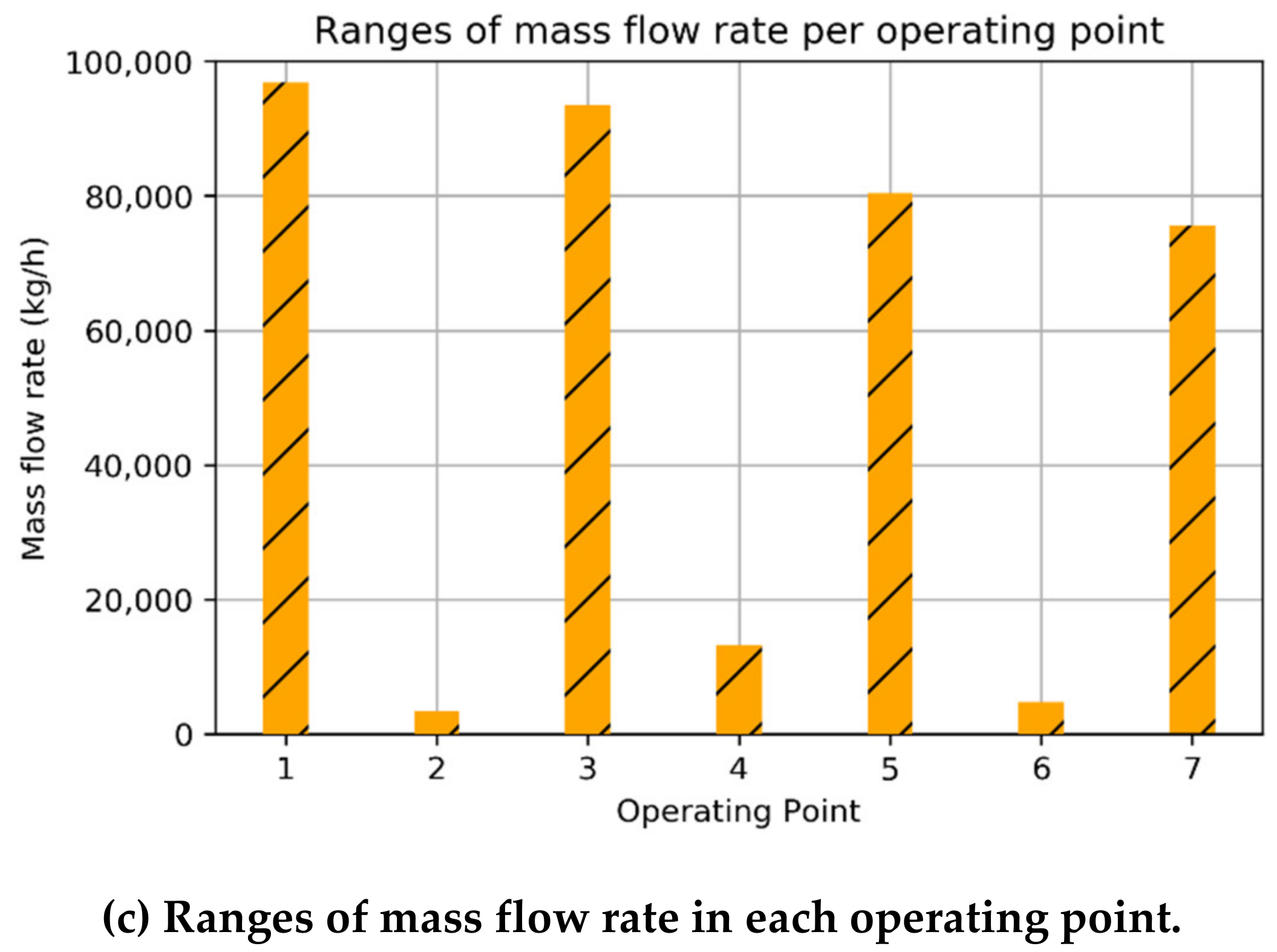
| Operating Point * | Temperature (°C) | Pressure (MPa) | Mass Flow Rate (kg/h) |
|---|---|---|---|
| 1 | 485–513 | 5.795–6.2 | 3835–96,789 |
| 2 | 283–365 | 0.08–1.565 | 0–3398 |
| 3 | 229–279 | 0.048–0.593 | 3835–93,521 |
| 4 | 229–279 | 0.048–0.593 | 0–13,202 |
| 5 | 229–279 | 0.048–0.593 | 3835–80,319 |
| 6 | 121–169 | 0.009–0.121 | 0–4772 |
| 7 | 28.616–100.02 | 0.00392–0.00561 | 3835–75,547 |
| Operating Point * | Temperature (Immersion Probes) [116] | Pressure (Pressure Transmitters) [117] | Mass Flow Rate (Differential Pressure Transmitters) [118] |
|---|---|---|---|
| 1 | Greisinger GTF 601-Pt100 | Yamatake JTG960A | Yamatake JTD960A |
| 2 | Yamatake JTG940A | ||
| 3 | Greisinger GTF 401-Pt100 | Yamatake JTD930A | |
| 4 | |||
| 5 | |||
| 6 | Yamatake JTD920A | ||
| 7 | Yamatake JTD910A |
| Operating Point | +/- | +/- | ||
|---|---|---|---|---|
| 1,4 (HPC) | 0.9914541639 | 0.02378781401 | 51.27713297 | 36.21271356 |
| 4,7 (LPC) | 0.9712139368 | 0.09161658705 | 36.22307872 | 50.75836187 |
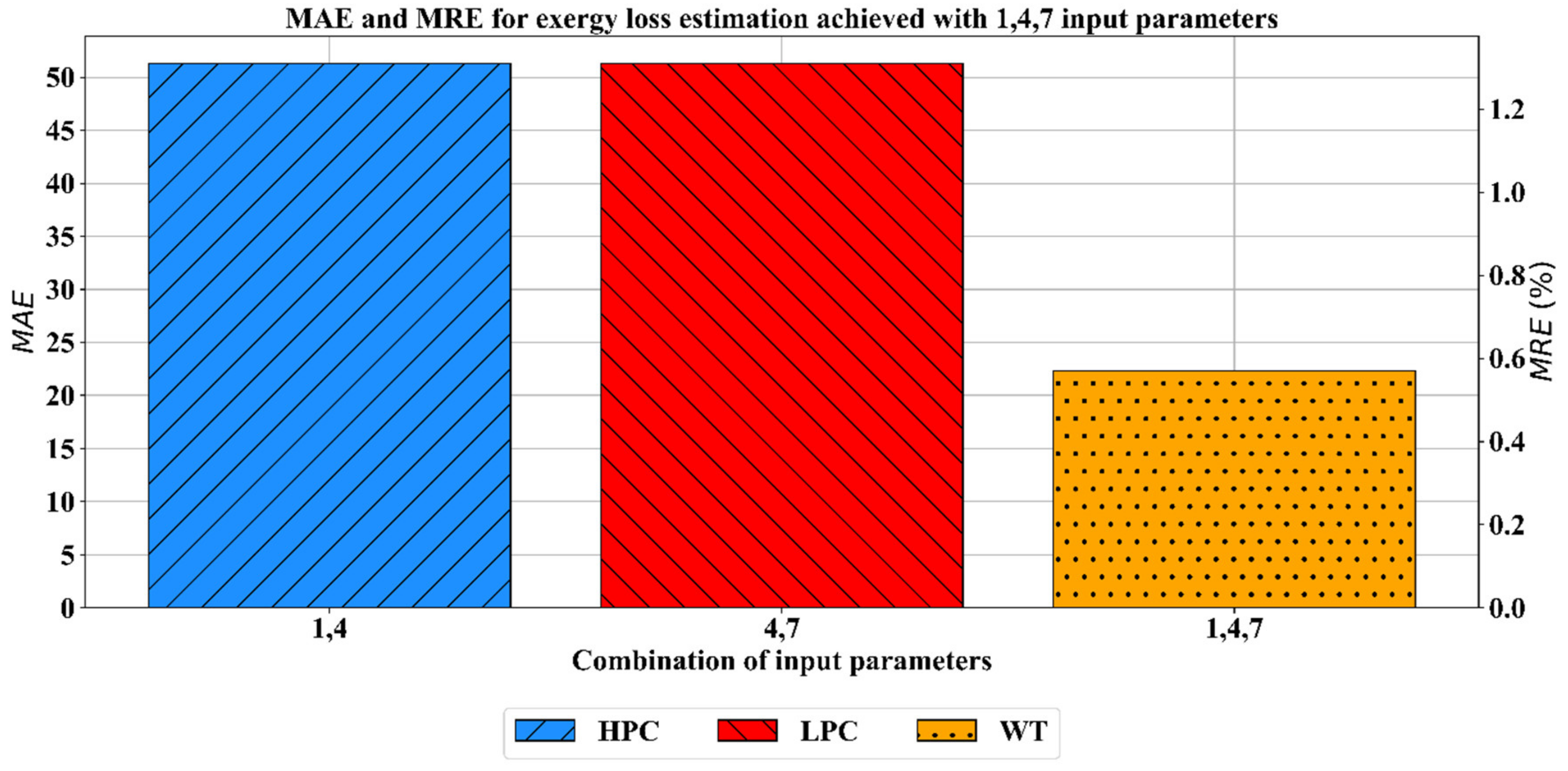
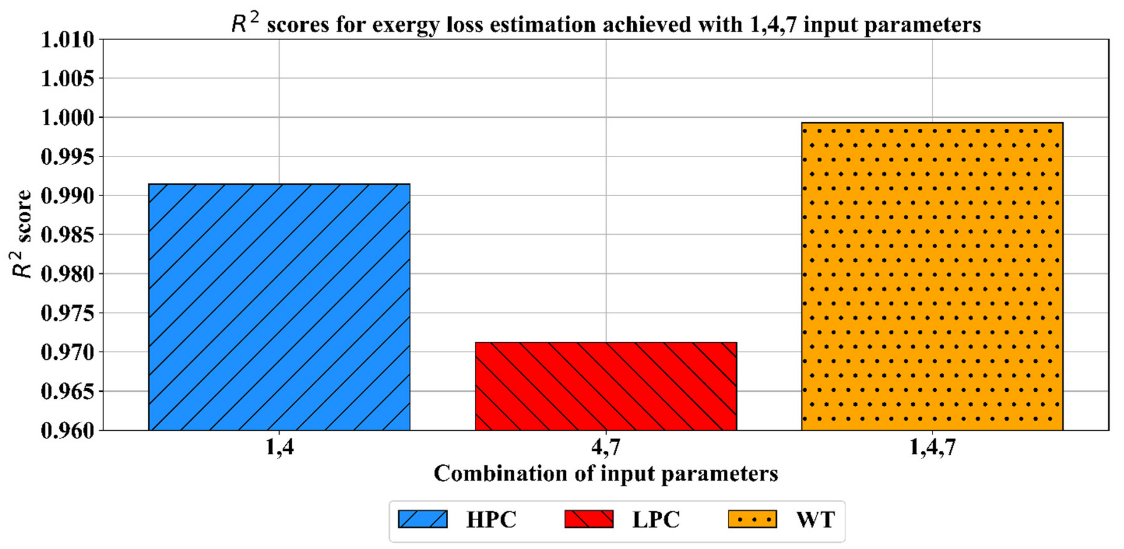
| 1,4,7 (WT) | 0.9992643028 | 0.00172978046 | 20.44955009 | 12.32598431 |
| Operating Point | 1,4 (HPC) | 4,7 (LPC) | 1,4,7 (WT) |
|---|---|---|---|
| Activation Function | ReLU | ReLU | ReLU |
| L2 Regularization | 0.001 | 0.01 | 0.1 |
| Hidden Layer Sizes | (84) | (84, 84, 84, 84) | (84, 84, 84, 84) |
| Learning Rate Type | Adaptive | Constant | Adaptive |
| Initial learning rate | 0.1 | 0.01 | 1e-05 |
| Solver | LBFGS | LBFGS | LBFGS |
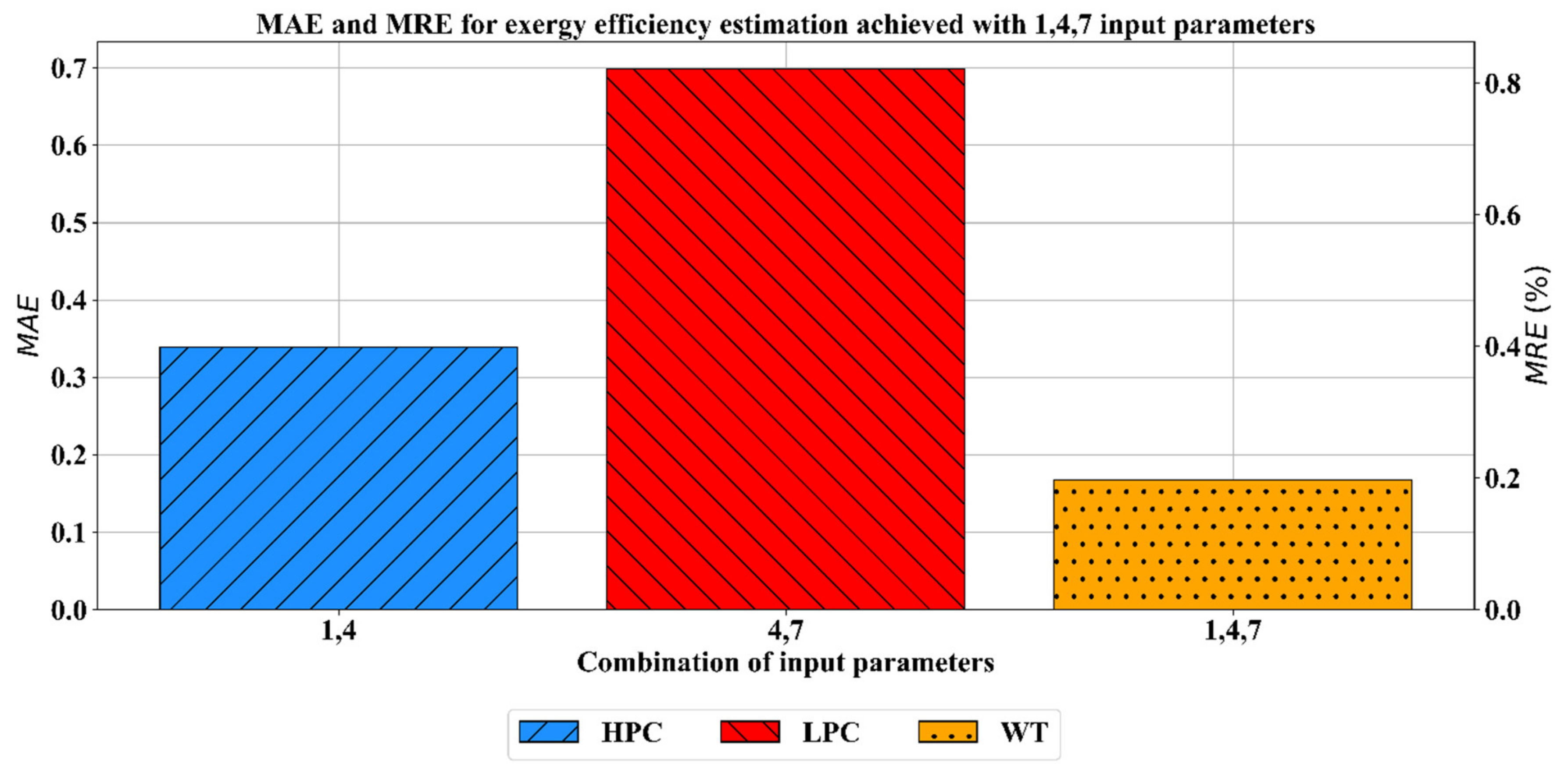
| Operating Point | +/- | +/- | ||
|---|---|---|---|---|
| 1,4 (HPC) | 0.9894154031 | 0.03141286439 | 0.3393632265 | 0.3058120431 |
| 4,7 (LPC) | 0.9906770758 | 0.02055184947 | 0.6985228666 | 1.1429986910 |
| 1,4,7 (WT) | 0.9951798924 | 0.01330619104 | 1.6066829045 | 0.0133061910 |
| Operating Point | 1,4 (HPC) | 4,7 (LPC) | 1,4,7 (WT) |
|---|---|---|---|
| Activation Function | ReLU | ReLU | ReLU |
| L2 Regularization | 0.1 | 0.1 | 0.1 |
| Hidden Layer Sizes | (84,42,21) | (84,84,84) | (84,84,84,84) |
| Learning Rate Type | Constant | Constant | Adaptive |
| Initial learning rate | 0.1 | 0.01 | 1e-5 |
| solver | LBFGS | LBFGS | LBFGS |
Publisher’s Note: MDPI stays neutral with regard to jurisdictional claims in published maps and institutional affiliations. |
© 2020 by the authors. Licensee MDPI, Basel, Switzerland. This article is an open access article distributed under the terms and conditions of the Creative Commons Attribution (CC BY) license (http://creativecommons.org/licenses/by/4.0/).
Share and Cite
Baressi Šegota, S.; Lorencin, I.; Anđelić, N.; Mrzljak, V.; Car, Z. Improvement of Marine Steam Turbine Conventional Exergy Analysis by Neural Network Application. J. Mar. Sci. Eng. 2020, 8, 884. https://doi.org/10.3390/jmse8110884
Baressi Šegota S, Lorencin I, Anđelić N, Mrzljak V, Car Z. Improvement of Marine Steam Turbine Conventional Exergy Analysis by Neural Network Application. Journal of Marine Science and Engineering. 2020; 8(11):884. https://doi.org/10.3390/jmse8110884
Chicago/Turabian StyleBaressi Šegota, Sandi, Ivan Lorencin, Nikola Anđelić, Vedran Mrzljak, and Zlatan Car. 2020. "Improvement of Marine Steam Turbine Conventional Exergy Analysis by Neural Network Application" Journal of Marine Science and Engineering 8, no. 11: 884. https://doi.org/10.3390/jmse8110884
APA StyleBaressi Šegota, S., Lorencin, I., Anđelić, N., Mrzljak, V., & Car, Z. (2020). Improvement of Marine Steam Turbine Conventional Exergy Analysis by Neural Network Application. Journal of Marine Science and Engineering, 8(11), 884. https://doi.org/10.3390/jmse8110884