Article

Cross-Shore Intertidal Bar Behavior along the Dutch Coast: Laser Measurements and Conceptual Model

1
Department of Hydraulic Engineering, Delft University of Technology, 2628 CN Delft, The Netherlands
2
Svasek Hydraulics, 3024 ES Rotterdam, The Netherlands
3
College of Earth, Ocean, and Atmospheric Sciences, Oregon State University, Corvalis, OR 97331, USA
4
Deltares, 2629 HV Delft, The Netherlands
*
Author to whom correspondence should be addressed.
J. Mar. Sci. Eng. 2020, 8(11), 864; https://doi.org/10.3390/jmse8110864
Submission received: 15 October 2020 / Revised: 28 October 2020 / Accepted: 29 October 2020 / Published: 31 October 2020
(This article belongs to the Special Issue Observation, Analysis, and Modeling of Nearshore Dynamics)

Abstract

:
Intertidal bars are naturally occurring morphological features along the waterline of sandy beaches. Present quantitative knowledge on intertidal bar behavior is limited, due to the scarcity of data resources and the limitations of traditional survey techniques. To investigate and quantify the cross-shore morphologic behavior of intertidal bars, hourly terrestrial laser scans of Kijkduin beach (The Netherlands) are used and a conceptual evolution intertidal bar model is constructed. In a six-week period in January and February 2017, a pronounced intertidal bar formed at Kijkduin beach and migrated onshore during mild wave conditions and eroded again during storm conditions. The observed maximum shoreward migration was 30 m horizontally with a maximum growth of about 1 m in the vertical direction. Onshore sediment transport fluxes peaked around 2 m3 per m width per day. In the conceptual model proposed here, run-up and overwash processes are dominant for shoreward growth and migration of the bar and submersion processes are responsible for bar destruction.

Graphical Abstract

1. Introduction

Seasonal intertidal sandbars are frequently occurring features on sandy beaches with a significant micro- and meso-tidal range [1] that often develop during mild wave conditions. They often occur when the coast is recovering [2,3] after the winter season transporting sand towards the coast (Figure 1) and ultimately creating a summer profile with a wider beach and steeper slope. During the storm season, storms often erode the beach-dune system [4] and a so-called winter profile is created with a relatively gentle slope and narrow beach. Seasonal bars differ from the (more permanent) multi-bar systems which occur on some coasts [1,5] with gentler slopes and larger tides.
Sediment underwater can be moved shoreward by the migration of subtidal and intertidal bars towards the beach [6]. The growth and migration of intertidal sandbars are driven by tide, surf zone, and swash-zone processes [7,8,9]. Ultimately, the bars weld to the beach above the water line [10] where the sand can dry. The dry sand can subsequently be transported by wind up to the dunes. The intertidal zone plays an important role in this shoreward sand transport because of high hydrodynamically driven onshore sediment transport rates [1,11] and the transition from hydrodynamic to aeolian sediment transports [12].
The growth, migration, and destruction of intertidal bars is controlled by many hydrodynamic and morphological mechanisms over multiple spatial and temporal scales [13]. This results in a complex coastal behavior that is hard to quantify and predict accurately. Wijnberg and Kroon [14] and Masselink et al. [1] concluded that the morphological behavior of an intertidal sandbar was largely dependent on the tidal water level and the nearshore wave conditions. Luijendijk et al. [15] concluded that tidal currents contributed little to the cross-shore sand distribution in the Netherlands based on numerical results around the Sand Motor.
Previous studies have used multiple observation techniques (such as airborne LiDAR [16,17], two-dimensional (2D) LiDAR [18], GNSS techniques [19,20], ultrasonic techniques [21,22], video techniques [23,24], and pressure sensors [25]) to obtain information in the intertidal zone. These measurements consist of point or areal measurements with varying temporal and spatial resolution and accuracy often obtained in time-intensive field campaigns.
Quartel et al. [23] identified (based on Argus video images [26]) cross-shore intertidal bar movements with a recurring period of one to four months. The following three phases were distinguishable in intertidal bar behavior: (I) generation around the low tide water, (II) landward migration, and (III) merging of the bar at the high waterline. Phases I and II were coupled to waves, but tide was not included, and no link was proposed for phase III.
Recent developments with continuous laser scanning [2,27,28] have provided the opportunity to study the intertidal area topography [8,29,30,31] with accurate high temporal-spatial measurements.
A long-range laser scanner using the LiDAR (Light Detection and Ranging) technique is, here, positioned at a fixed location overlooking the beach. A command computer equipped with a scheduler is used to obtain regular scans of the beach with (time) varying resolution settings.
In this article, we present a six-week laser scan (cross-section) analysis of the complete development and destruction cycle of an intertidal bar on a meso-tidal beach at Kijkduin beach, in the Netherlands. Subsequently, a conceptual evolution model is presented that describes the different stages of the observed development and destruction of an intertidal bar and the relative contributions of waves and tide to the development. Previous studies [31,32,33,34] have indicated that waves and tides were important drivers for the intertidal bar behavior, but up to now no clear model has been identified.

2. Field Site Kijkduin

2.1. Field Site

In 2016, the CoastScan project started aiming to provide detailed LiDAR measurements of the beach and dunes on multiple spatiotemporal scales [28]. A measuring station was setup at Kijkduin in the Netherlands to monitor a km of beach for up to six months from November 2016 to June 2017. Hourly topography was obtained using a Riegl VZ 2000 laser with an accuracy in the order of cm. Figure 2 gives an overview of the beach and dunes in relation to the position of the laser scanner.
The area contains a sandy beach and a dune area with quartz sand with a median grain size (D50) of 300 μm [35]. Depending on the season, patches of shells are found on the surface. The study area is exposed to an episodic seasonal wave climate.
Average wave heights are around 1.7 m with small waves (Hs < 1 m) predominately from the NW, average waves (1.5 m < Hs < 4.5 m) from the SW-NW and high waves (Hs > 4.5 m) originating from the W-NW direction [15]. Tides around Kijkduin are semidiurnal and asymmetric (rising period of 4 h 20 m and a falling period of 8 h) with a spring/neap tidal range of about 2.4/1.5 m.

2.2. Laser Scans of Intertidal Topography

A total of 82 low water scans (15 January to 28 February with a gap around 22 February, due to an acquisition error) with a resolution of 0.05° × 0.05° degree are used in the current analysis. The selected cross-section (see Figure 2) is located at the center of an intertidal sandbar, where longshore changes are expected to be minimal. Moreover, the selected cross-section is located relatively far away from a subtidal runnel which might influence the cross-shore intertidal behavior.
Data were processed in a five-step procedure, visually represented in Figure 3. As a first step, data were georeferenced and aligned based on three ground control points (GCP, see Figure 2 and Figure 4) [36,37]. These GCPs consisted of a building wall to the south of the scanner and two information signs in the dunes. The alignment correction angles were determined by minimizing the distance between the GCP’s of the first and subsequent nth scan with nonlinear regression [38]. After cropping of the scan around the cross-section, the data were cleaned from noise and objects with the LasTools software [39]. A box (step) size of 2 m and isolated point count threshold of eight was used for the noise. As a final step, the data were interpolated to fill in any gaps and to obtain the cross-sections.
Initial results still showed variations in the beach height of about 5 cm at stable objects [28]. The limited number of useful georeferenced objects along the Kijkduin coast caused the used method to be less accurate. For analysis of the intertidal zone, all the profiles were further corrected by aligning the height of the berm, along a 12 m stretch, to the average height, as observed variations at that point were assumed to be minimal.

2.3. Wind and Water Data

Environmental data were acquired from various sources. Wind data were obtained from the Dutch Meteorological office [40] at Hoek van Holland (HVH, 15 km south of Kijkduin, Figure 5) and tidal elevations were obtained from the Ministry of Public Works [41] at Scheveningen (2 km north of Kijkduin). Wave data [41] were available from two wave buoys at IJmuiden ammunition storage (IJM MSP) and Europlatform (EUR) located about 45 km NNW and WSW from Kijkduin.
In order to obtain local wave information at Kijkduin, the wave model Delft3D-Wave [42] was used. According to the Sand Engine model [15], a double nested wave model was constructed to estimate the wave properties at 3 m (mean sea level) water depth in front of Kijkduin. Wave boundaries were obtained from the IJM MSP (north side), EUR (south side), and interpolated IJM MSP-EUR results along the west side. Wind data, from Hoek van Holland, were uniformly applied over the grid area and tidal data, from Scheveningen, were used for water levels (i.e., tidal currents were not calculated). The model was run time dependent with a time step of 15 min.
To obtain an estimation of the maximum local wave setup and run-up due to incident and infragravity waves, the 2% exceedance value of run-up peak at Kijkduin beach [43] is calculated with:
R 2 = 1.1 ( 0.35 β HL + 0.5 HL ( 0.563 β 2 + 0.004 )
where H is the wave height (in m) in deep water, L = gT2/2π the wavelength (in m), and T the peak wave period (in seconds) in deep water. For the deep-water values, a separate output location in front of Kijkduin, at 15 m water depth, was included in the Swan model. The average beach steepness β of 0.0129 in front of the cross-section was calculated based on depths from the swan grid.
Figure 6 shows the calculated wave data at Kijkduin in the period from 15 January to 28 February 2017. It shows the wave height and wave peak period next to the local wind conditions (wind speed and wind direction), the local tidal elevation, and the tidal range and run-up. Results will further be discussed in the next section.

3. Results

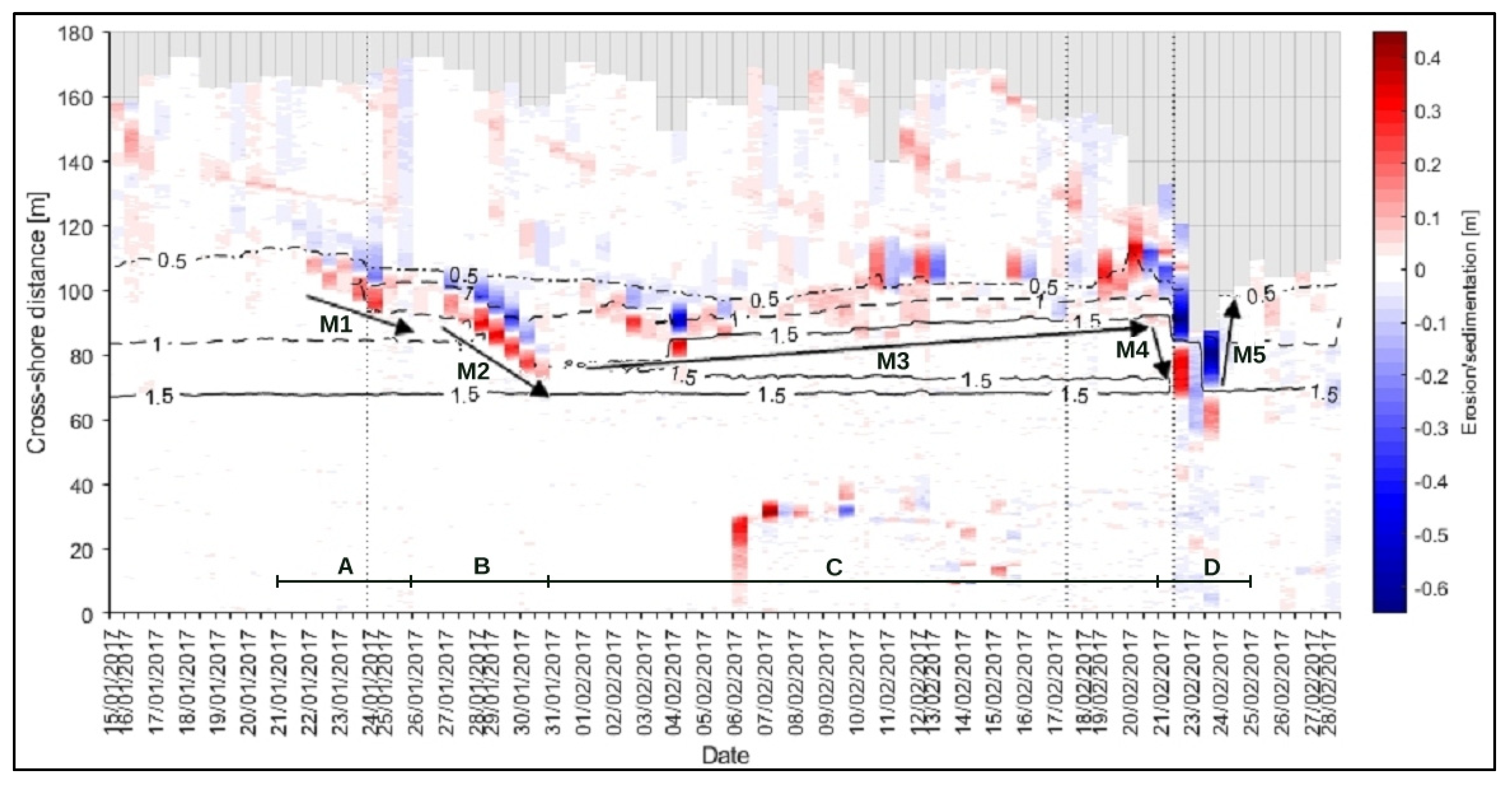
3.1. Intertidal Bar Cycle

A pronounced intertidal sandbar develops, grows, migrates, and was destroyed in the period from 15 January to the end of February 2017. Figure 7 shows a subset of 7 out of the 82 available low water scans, indicating the most pronounced changes. Initially, the bed level shows a relatively smooth parabolic shape from the low water line up to the berm. Starting with a small perturbation, the sandbar quickly develops in about five days (Movement 1, here after referred as M1) raising the height 0.7 m (+0.5 m to +1.2 m NAP), while moving onshore over a distance of 10 m (x = 110 m to x = 100 m). In the next five days (M2), the crest moves about 25 m (x = 100 m to x = 75 m) raising the height 0.3 m (+1.2 m to +1.5 m NAP), while the movement dampens in the following 20 days (M3). Just before the storm on 24 February hits the coast, a short and rapid onshore movement and elevation of the crest is visible (M4). Finally, the intertidal sandbar is leveled by the storm recreating the smooth parabolic beach shape (M5). At the end of this period, no significant sedimentation of the upper intertidal zone took place due to bar welding.
Figure 8 shows a sedimentation and erosion stack plot based on all available low water scans, where the height differences per tidal cycle in the cross-shore direction are derived. Despite some missing low water periods (indicated with a vertical dotted line), sedimentation and erosion patterns are clearly visible in time. The distinctive intertidal-bar changes (Figure 7) can be observed in the stack plot (Figure 8), indicated by the arrows identifies as M1–M5. Especially, the strong onshore movement from 26 January to 31 January (M2) and the destruction of the bar (M5) around the 24 February is clearly visible. The widening of the bar is, except from two or three clear occurrences, less visible.
The intertidal bar behavior, around M1–M5, is studied in more detail in the next sections. For convenience, the detailed study is performed during three periods of about five days (21–26 and 26–31 January (M1 and M2) and 21–26 February (M4 + M5)) and one period of 21 days (1–20 February (M3)), as indicated in Figure 7.

3.2. Detailed Intertidal Bar Behavior

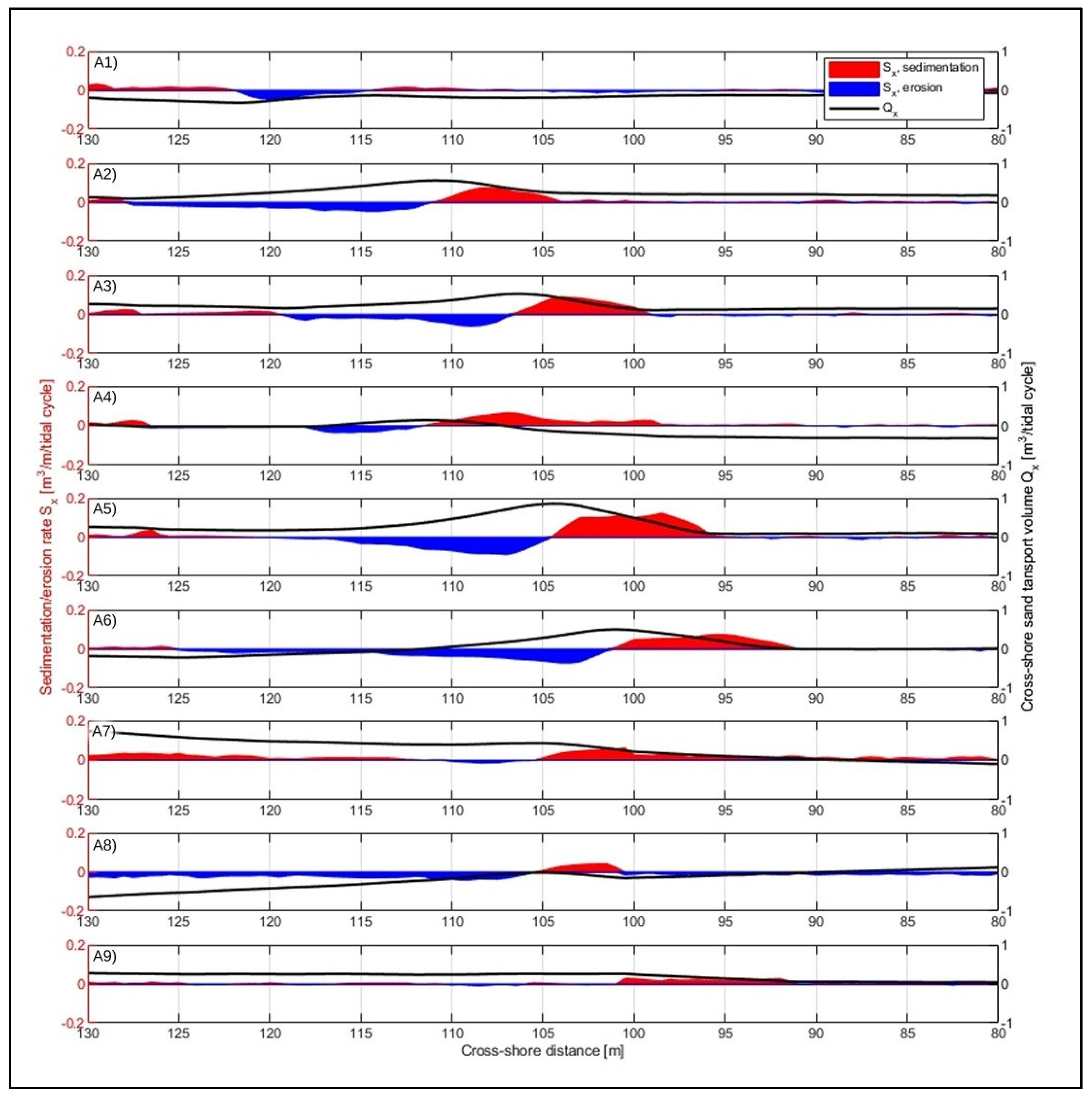
3.2.1. Period A: Initial Bar Development (M1)

The initial bar development from 21–26 January is shown in Figure 9. The bar develops from a small ripple to a height of about half a meter and moves about 10 m onshore. The total water line (here defined as the high tide elevation plus setup and the run-up) analysis, visualized with the dashed dotted lines in Figure 9, indicates that the highest water level occurs after each low water, and shows that the tidal water level does not rise above the bar crest. During this period, light onshore (3–5 m/s) and stronger offshore (up to 9 m/s) winds result in small (calculated) offshore wave heights (see Figure 6) ranging from 0.6 to 0.1 m, with run-up up to 0.2 m. The tidal elevations in Figure 6 show a slowly increasing tidal range.
In a two-dimensional situation without alongshore sediment transport, the change in bed height and the cross-shore sand transport can be calculated using the mass continuity equation as expressed in the formula:
dh dt = S x 1 ϕ = 1 1 ϕ Q x x
where h represents the height of the bed, Sx the sedimentation/erosion rate, and Qx the cross-shore sand transport at a specific location along the cross-section. The porosity ϕ is assumed constant and equal to 0.4.
Integrating the sedimentation/erosion volumes starting at the onshore boundary results in an estimation of the sediment transport volume (Qx) in cross-shore direction. Figure 10 shows the sedimentation/erosion volumes (Sx) for nine tidal cycles between 21 and 26 January. Sedimentation/erosion volumes (Sx) reach up to 0.15 m3/m per tidal cycle, depending on the cross-shore location and time. During about half of the nine tidal cycles, a clear net incoming sediment transport is visible at the seaward side of the domain (where Qx > 0). The fifth and sixth tidal cycles contain the largest incoming sediment flux (Qx) at the seaward boundary of the domain, i.e., up to nearly 0.9 m3 per m width in a tidal cycle.

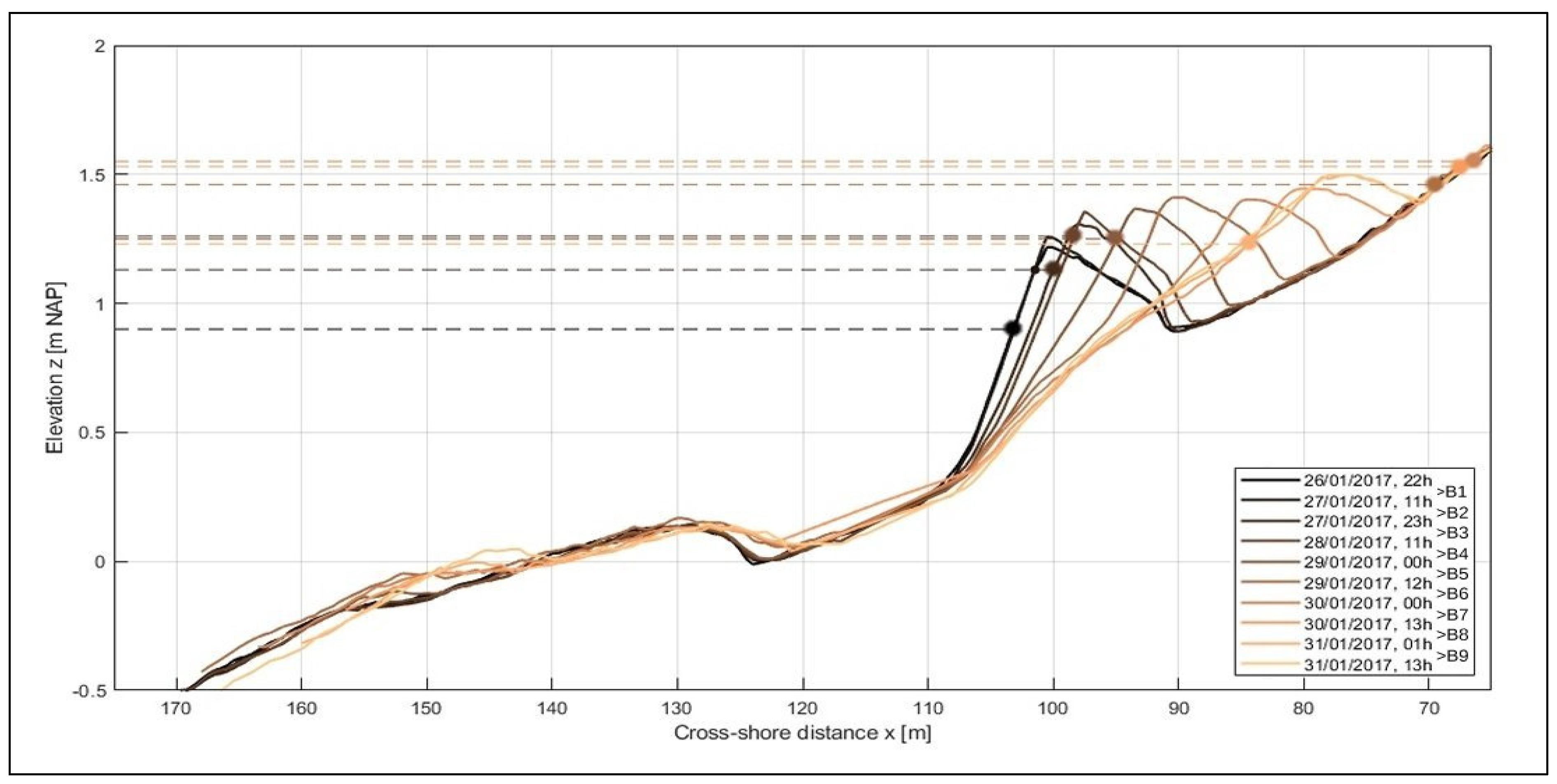
3.2.2. Period B: Onshore Bar Migration (M2)

The fast-onshore intertidal bar movement from 26 to 31 January is shown in Figure 11. The bar moves around 25 m onshore and flattens during this process. Initially, the derived total water level just reaches below the top coinciding with a peaky crest and once it is over the crest, the bar becomes smoother. Winds up to 8 m/s are mostly offshore, and calculated wave heights grow from about 0.1 to 0.7 m in this period, with run-up reaching about 0.2 m. The tidal elevations show an increase in the tidal range.
Figure 12 shows the sedimentation/erosion volumes (Sx) for nine tidal cycles between 26 and 31 January. Volumes (Sx) reach up to 0.2 m3/m per tidal cycle, depending on cross-shore location and time for both sedimentation and erosion. During most of the nine tidal cycles, a clear net incoming sediment flux is visible at the seaward side of the domain (Qx > 0). The fourth and fifth tidal cycles contain the largest onshore flux (Qx) around the tidal bar of up to nearly 1.1 m3 per m width in a tidal cycle.

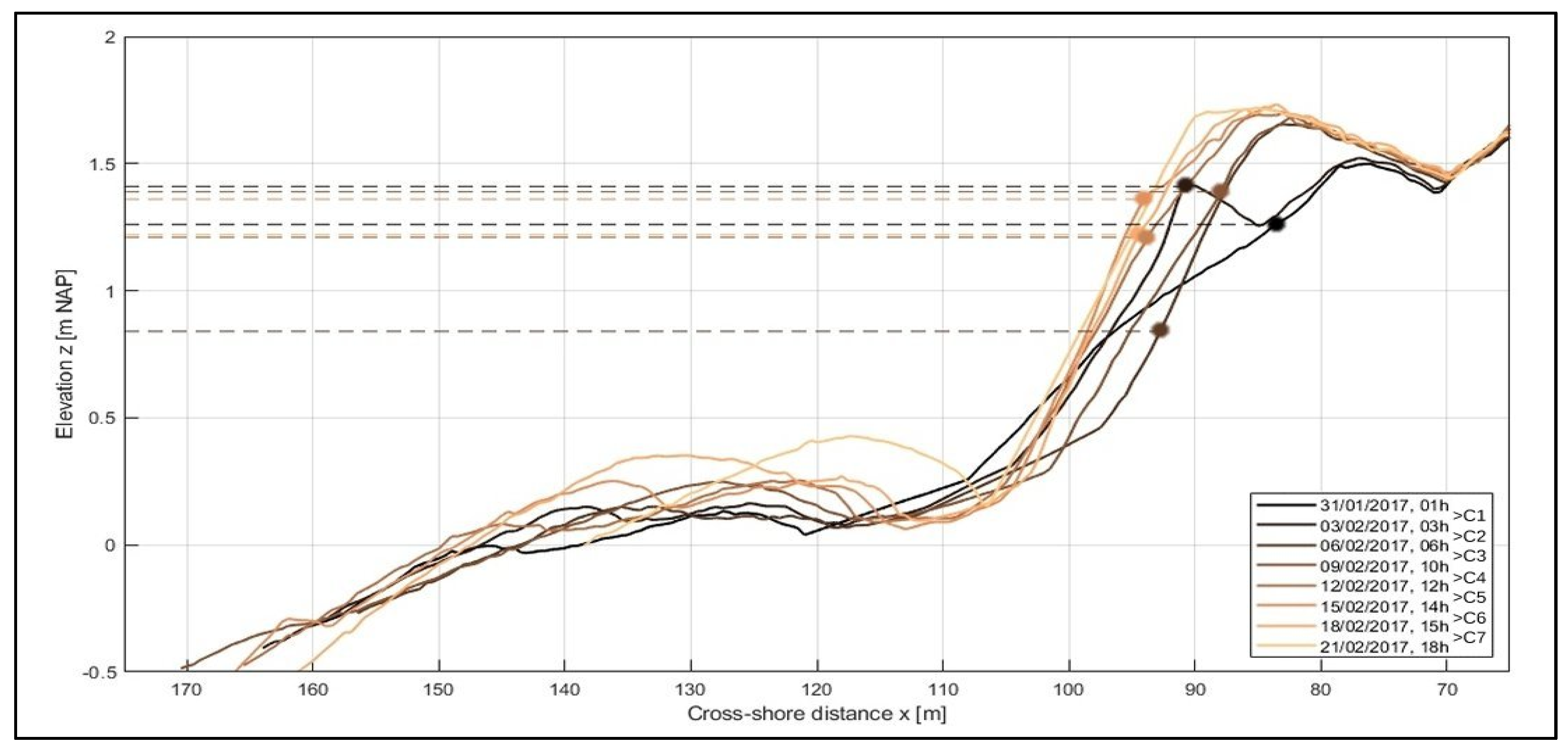
3.2.3. Period C: Horizontal and Vertical Growth (M3)

Figure 13 shows the gradual growth of the bar over 21 days (31 January to 21 February) more than doubling the volume of the bar. Except for some peaks, the growth of the bar is really slow. Wind and wave conditions are variable during the 21 days, with wave heights not exceeding 0.7 m and wind speeds under 10 m/s. Tidal variations in this period are more erratic with a less clear spring and neap tide cycle.
Tide-to-tide analysis has proven to be difficult during this period due to the small daily height changes which are within the estimated errors of the laser scanner. Figure 13 shows the evolution of the bar every three days (six tidal cycles), with the calculated sediment transport volumes based on these three-day differences.
Figure 14 shows the sedimentation/erosion volumes (Sx) for seven three-day cycles between 31 January and 21 February 2017. Transported volumes (Sx) reach up to 0.01 m3/m per tidal cycle depending on cross-shore location and time for both sedimentation and erosion. During more than half of the seven cycles, a clear net incoming sediment is visible at the seaward side of the domain (where Qx > 0).

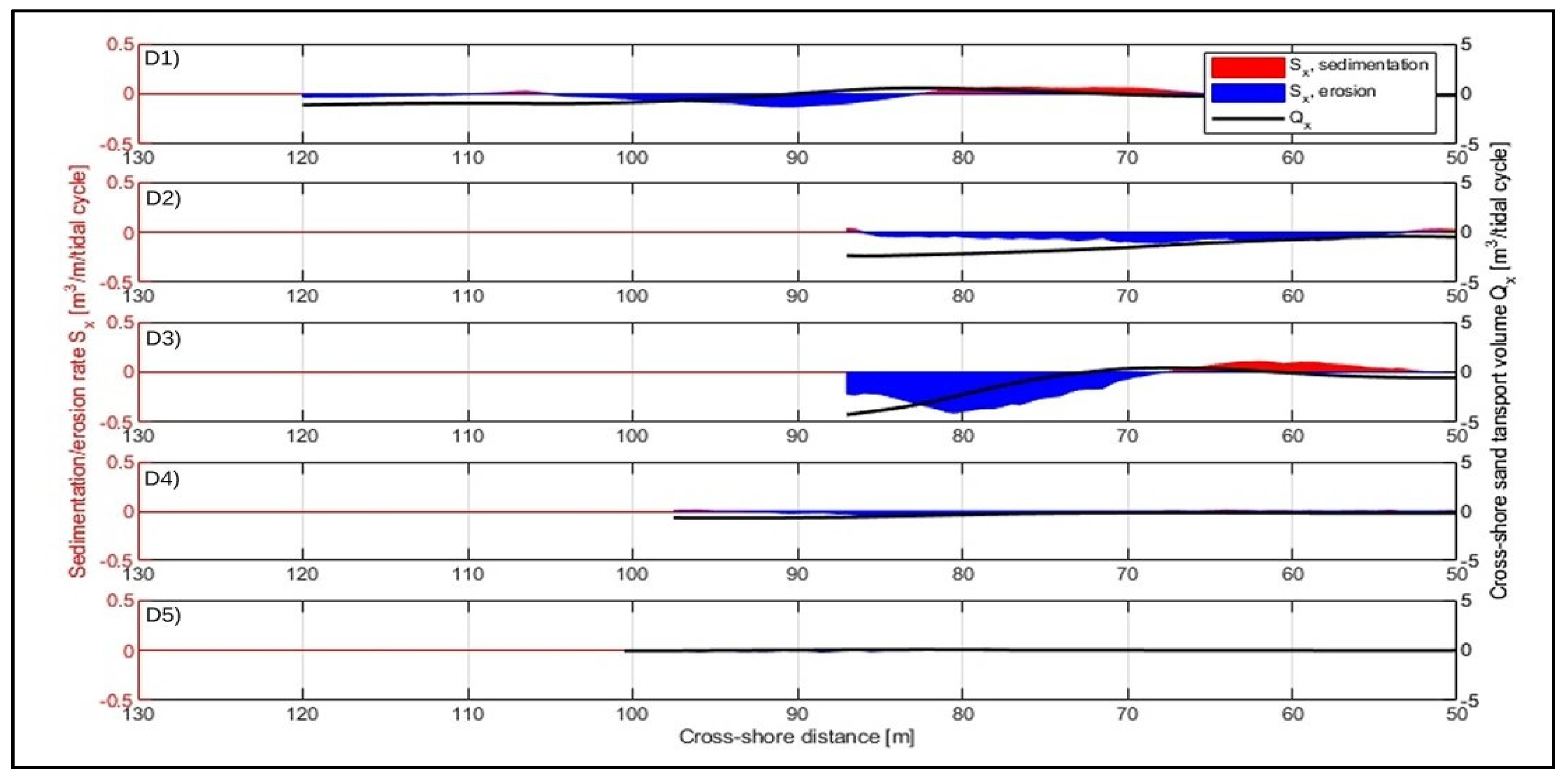
3.2.4. Period D: Shoreward Movement and Bar Destruction (M4 and M5)

Figure 15 shows the final stages, up to the leveling of the beach around 24 February. After a 10 m shoreward movement of the bar, the bar was destroyed during the night on 24 February, with winds up to 20 m/s and wave heights of nearly 2 m, and run-up values of more than half a m. Unfortunately, scans on 22 February were not available (due to a laser scan malfunction) resulting in a gap in the available data of the final shoreward movement of the intertidal bar. The relatively high water level at low tide on the evening of 23 February also resulted in limited information on the bar around that time.
The destruction of the bar shows sedimentation/erosion volumes of up to 0.4 m3/m per m width (see Figure 16), which is a doubling as compared with the observed volumes in the previous periods (A–C). The offshore flux (Qx) reaches 4 m3 per m width in a single tidal cycle.

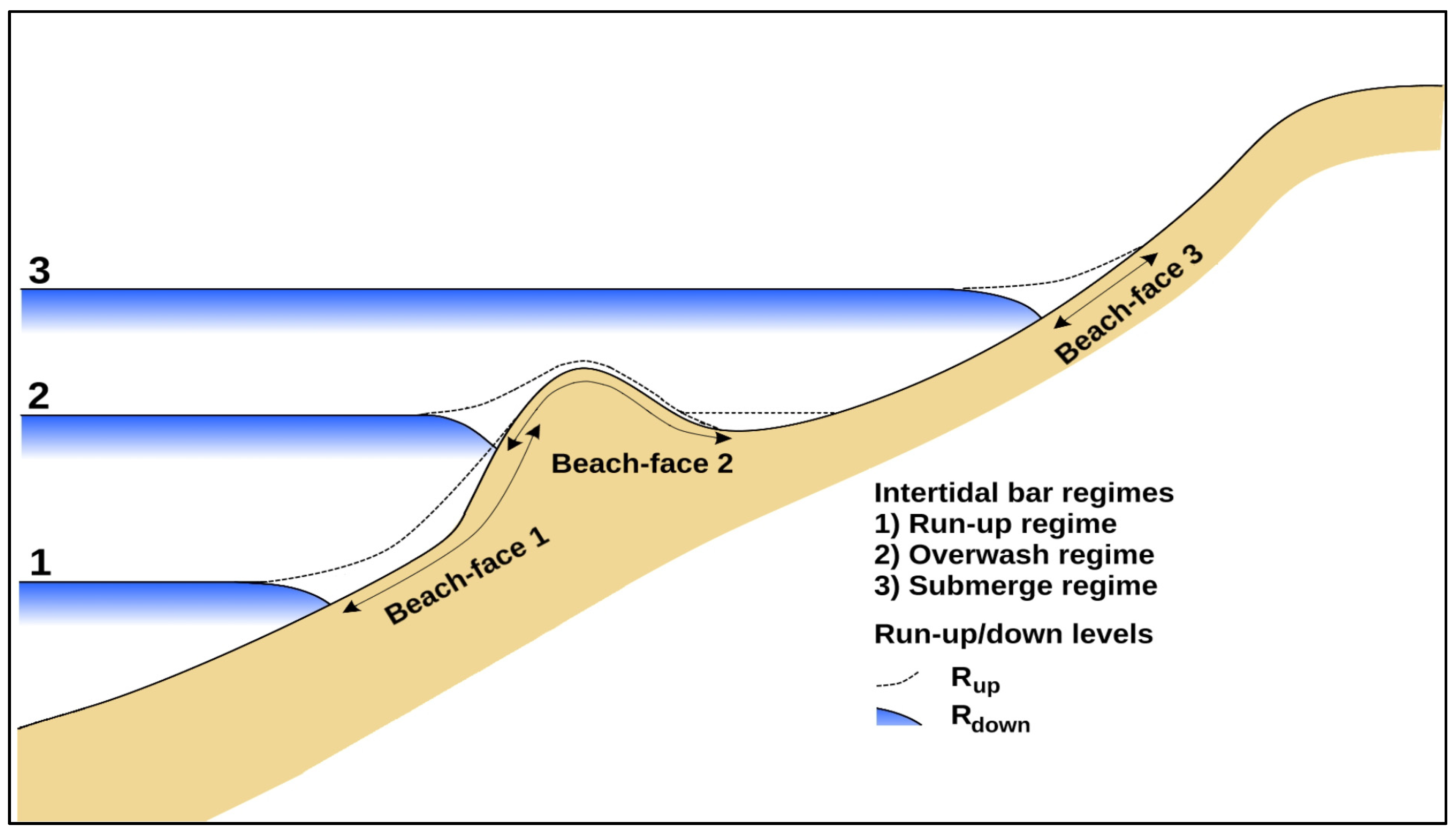
4. Conceptual Intertidal Bar Behavior Model

In order to interpret and to better understand the observed results, a conceptual model is developed and used in an effort to generalize the observed intertidal bar measurements. The model builds upon the work of Quartel et al. [23] who had already identified several phases of shoreward intertidal bar behavior. The CoastScan data provides a high-resolution description of the entire cycle from the development, growth, shoreward movement, and destruction of the intertidal bar. The model is based on two-dimensional (2D) cross-shore behavior and lacks three-dimensional (3D) variability.
Depending on the water level with respect to an intertidal bar crest elevation, both surf zone and swash-zone processes can be dominant for the morphological behavior. For the conceptual model developed here, this relative water level is categorized into the three intertidal bar regimes as presented in Figure 17 and inspired by the storm impact regimes proposed by Sallenger [44]. During relatively low water levels, the run-up regime prevails, where the run-up level (Rup) remains below the bar crest. When the relative water level increases and the run-up level gets above the bar crest, the overwash regime is reached. Swash-backwash processes [1,14,45] are identified in this regime as driving forces for the generation and shoreward movement of the bars. Finally, for a relatively high water level, the submersion regime prevails, when the rundown level is also above the bar crest. For energetic wave conditions, the beach face, then, tends to be flattened due to a strong undertow, resulting in a net offshore sediment transport [6,45].
The nearshore wave heights (here at 3 m water depth) are classified as mild (Hs < 1.5 m) and energetic (Hs > 1.5 m) conditions, respectively. This distinction at 1.5 m is based on Kroon et al. [46], and Luijendijk et al. [15] who indicated that higher waves had a significant morphological influence on the Dutch coast.
In the laser measurement results at Kijkduin beach, five distinctive intertidal bar movements (M1–M5 as seen in Figure 7) were observed. In these movements, four development stages are recognized, i.e., formation, migration, growth, and destruction. The formation, migration, and growth occurred during mild wave conditions, while the destruction of the intertidal bars occurred during energetic (storm) wave conditions. Within a regime, the wave conditions in the surf zone and the swash zone, together with the local bathymetry and the sediment characteristics, determine the magnitude and direction of sediment transport based on the dominant cross-shore sediment transport processes.
Combining the observed intertidal bar behavior with the wave conditions, the conceptual model of the intertidal bar behavior at Kijkduin beach is presented in Table 1. The five observed intertidal bar movements (see Figure 7) are classified in this model and indicated by the circled numbers. The conceptual model is explained and described below for each development stage.
A. Formation
Initially, when no intertidal bar is present, the three intertidal bar regimes are not distinguishable. For mild wave conditions, the beach face tends to steepen, where the net onshore sediment transport is dominant. Results by Vos et al. [30] (see Figure 4) indicated that the intertidal bars originated around the 0.5 m NAP line, in the upper reaches of the tidal range. When the daily tidal range was insignificant (i.e., <1 m, according to Masselink et al. [1]), for example, during neap tide, the bar did not move. The wave action merely resulted in an equilibrium profile where the beach face was relatively steep and a beach berm was created, as depicted in Figure 18a. Once the tidal range was or became larger (i.e., >1 m, according to Masselink et al. [1]), for example, towards spring tide, the bar could move shoreward.
The duration of the wave action at one location, in other words, the residence time for cross-shore sediment transport processes to occur [1,7], is important for the formation of the intertidal bar. As described above, an insignificant tidal range (i.e., <1 m) does not support the formation of a moving intertidal bar.
B. Migration
With increasing tidal range (i.e., > 1 m), an intertidal bar can move up the beach, as depicted in Figure 18b and Figure 11. With an increasing water level, the wave action moves up along the beach profile. An (fast) onshore migration may occur in the overwash regime due to swash-zone processes, as observed in the laser measurements (movements M2 and M4). Waves overtop the bar when the still water level is just below the bar crest elevation. Sediment is transported over the crest by wave-breaking induced turbulent uprush changing to gravity induced backwash on the landward site of the bar. Where generally these two processes (uprush and backwash) counteract each other, in the overwash regime, they are complementary. This can result in a fast-onshore migration (Figure 11). The water that overtops the bar crest infiltrates the soil or flows back offshore through trough/rip channels (3D effect). For energetic wave conditions, the bar crest might be eroded due to high flow velocities, changing from the overwash to the submersion regime.
C. Growth
In the run-up regime, the intertidal bar can grow horizontally, widening the bar (observed movement M3 in Figure 13). During mild wave conditions, sediment (in the form of small amplitude bars) can migrate onshore by surf- and swash-zone processes. In the run-up regime, this sediment transport may feed the existing intertidal bar, by welding to the seaward slope due to swash-zone processes, as observed in the laser measurements (movement M3).
In the overwash regime, the intertidal bar can grow horizontally and vertically (observed movement M3 and M4). Horizontal growth occurs due to surf- and swash-zone processes. Sediment transported onshore feeds the seaward slope of the bar or is transported further, resulting in vertical growth of the intertidal bar due to swash-zone processes. When flow velocities on the bar crest are small, sediment advected from the surf zone and stirred in the uprush settles and increased the bar height.
In the submersion regime, no significant growth is expected. When the intertidal bar is submerged, the surf zone processes are prevailing. Flow velocities are usually relatively large over the bar crest as the water depth is relatively small. Therefore, it is unlikely that sediment will settle on top of the bar crest.
D. Destruction
The destruction of the intertidal bar occurs during energetic wave conditions [47,48] (see Figure 15). In the run-up regime, the destruction of the intertidal bar might occur due to sediment eroding on the seaward slope of the bar. When a critical slope angle is exceeded, sediment slumps down, resulting in the destruction of the intertidal bar. In the overwash regime, flow velocities over the crest can be large for energetic wave conditions. Sediment gets stirred in the water column, thereby, decreasing the bar height. Finally, when reaching the submersion regime, the intertidal bar can be destructed rapidly under energetic wave conditions. Under these conditions the undertow becomes dominant, resulting in a strong offshore sediment flow, especially above the bar crest where the water depth is relatively small.

5. Discussion

The accuracy of the laser measurements has proven to be satisfactory to study the marine driven intertidal behavior. Compared with other studies, the laser scanner allows for measurements with higher accuracy (compared with, for example, automated Argus video methods [24,49]) and higher spatiotemporal resolutions (compared with, for example, GNSS surveys [10]).
The cross-shore interpolation of the selected cross-section induced some interpolation errors due to missing data and the use of linear interpolation techniques. The missing data can be attributed to the existence of water draining runnels, areas that are too wet to detect or areas that are in the shadow zone of the laser scanner (from, for example, vehicles or persons). Small gaps and runnels could easily be covered with linear interpolation.
On average, the measured tidal bar behavior is similar to other locations. Kroon [45], Jensen et al. [50], and Cohn et al. [51] found similar formation-migration-destruction intertidal bar behavior along the Dutch, Danish, and USA coast with bar heights between 0.4 and 1.2 m and migration speeds up to 12 m a day. Other researchers, for example Dawson et al. [52] and Cohn et al. [53] found migrating bars with relative slower speeds of 1–2 m a day. Tidal and wave conditions varied from location to location and were not directly connected to tidal bar properties.
Most known sediment transport rates (see reviews of Blenkinsopp et al. [54] and Masselink et al. [22]) are based on a swash-to-swash basis and reach up to 175 kg/m in the surf zone. These are not easy to compare with the tidal CoastScan data, due to the different timescales (min as compared with tidal periods of 12 h) and a lack of integrated results. Blenkinsopp et al. [54] also provided sediment transport rates per tidal cycle at one location in the order of O(100)–O(1000) kg/m per tide. These values were smaller than the calculated sediment transport rates based on the CoastScan data. The maximum observed shoreward sand transport rate of 1.1 m3/m and seaward sand transport rate of 4 m3/m per tidal cycle gives around 2200 (shoreward)–6800 (seaward) kg/m with an average sand density of 1650 kg /m3 (local sample).
Brand et al. [31] found a relation between daily intertidal beach volume change and suspended transport rate in the surf zone. However, without detailed wave or bathymetry measurements (in the form of swash-to-swash bathymetry, similar to Blenkinsopp et al. [54]) it is not possible to compare the CoastScan sediment transport rates with transport rates on different time scales.
The conceptual model was mainly developed on the observed seasonal intertidal behavior at Kijkduin with additions from the literature. We think that the model is also applicable for similar sand beaches in other locations. Aagaard et al. [55,56], Cohn et al. [10], Quartel et al. [23], Uunk et al. [24], and van Maanen [57] saw similar results in micro- and meso-tidal beaches with similar hydrodynamic conditions in the Netherlands, Denmark, New Zealand, and the USA. However, different intertidal bar behaviors have been observed on macro-tidal beaches (Belgium [31]) and France [58]) where the relation between intertidal bar behavior and wave/tide forcing was less clear. A large tidal range results in shorter wave action duration at one location. Therefore, the formation process, possibly, cannot catch up with the rising tide. Consequently, the area is submerged, and different sediment transport processes become dominant [1,5].
Future challenges lie in obtaining long-term swash-zone hydrodynamic boundary conditions for intertidal morphological modeling with Xbeach [59] and expanding the conceptual model with 3D variability.

6. Conclusions

An intertidal bar, at Kijkduin Beach, was monitored during its six-week development and destruction during January and February 2017. Five different stages were identified from initial conception, growth, migration, widening, and the ultimate destruction.
A total of 82 low tide terrestrial laser scans were used to monitor the development of the intertidal bar. The maximum observed horizontal movement of the intertidal bar was about 30 m. with a maximum growth of about a m in height during a single tide period. Observed bed level changes enabled the determination of intertidal cross-shore sediment fluxes and the total sediment transport. The maximum observed erosion/sedimentation fluxes, S, reached about 0.2 m3 per m in a tidal period and a total sediment transport, Qx, of 1.3 m3 during the constructive phase of the bar. During the destructive phase, sediment fluxes reached up to 0.4 m3 per m and the total transport exceeded 4 m3 per m per tidal period.
A conceptual model of intertidal bar behavior, at Kijkduin, was developed which coupled the different stages in the development and destruction of the bar to the two main driving forces, i.e., waves and tides. Five different stages were defined which could be linked to specific circumstances. The conceptual model shows that the initial growth can largely be explained by sediment transport due to run-up processes. With increasing tidal range and moderate wave heights, run-up and overwash processes push the intertidal bar up the beach. Further vertical growth is the result of a combination of run-up and overwash processes, while the widening of the bar is attributed to run-up processes. The destruction of the intertidal bar is attributed to the submersion regime, where the intertidal bar is completely flooded and destroyed by the strong undertow return flows.

Author Contributions

Conceptualization, S.V.; methodology, S.V., L.S., and S.d.V.; software, S.V., L.S., and R.H.; validation, S.V. and L.S..; formal analysis, L.S. and S.V.; investigation, L.S. and S.V.; resources, S.V.; data curation, S.V.; writing—original draft preparation, S.V. and L.S.; writing—review and editing, S.V., R.H., A.R., R.M., and S.d.V.; visualization, L.S. and S.V.; supervision, S.d.V. and A.R.; project administration, S.d.V.; funding acquisition, S.V. and S.d.V. All authors have read and agreed to the published version of the manuscript.

Funding

The work in this article was financed by the ERC-advanced grant 291206 Nearshore Monitoring and Modeling and the CoastScan project 2018/STW/00505023.

Acknowledgments

The authors wish to thank the owner and manager of the Hotel NH Atlantic Den Haag (www.nh-hotels.nl) for supporting the research through the use of the hotel for the measurements. Additional thanks go to Baars-CIPRO (www.baars-cipro.nl) for advice and the construction of the measuring frame and operational support.

Conflicts of Interest

The authors declare no conflict of interest.

References

  1. Masselink, G.; Kroon, A.; Davidson-Arnott, R. Morphodynamics of intertidal bars in wave-dominated coastal settings—A review. Geomorphology 2006, 73, 33–49. [Google Scholar] [CrossRef]
  2. Phillips, M.S.; Blenkinsopp, C.E.; Splinter, K.; Harley, M.D.; Turner, I.L. Modes of Berm and Beachface Recovery Following Storm Reset: Observations Using a Continuously Scanning Lidar. J. Geophys. Res. Earth Surf. 2019, 124, 720–736. [Google Scholar] [CrossRef]
  3. Brooks, S.M.; Spencer, T.; Christie, E. Storm Impacts and Shoreline Recovery: Mechanisms and Controls in the Southern North Sea. Geomorphology 2017, 283, 48–60. [Google Scholar] [CrossRef] [Green Version]
  4. Splinter, K.; Strauss, D.; Tomlinson, R.B. Assessment of post-storm recovery of beaches using video imaging techniques; A case study at Gold coast, Australia. IEEE Trans. Geosci. Remote. Sens. 2011, 49, 4704–4716. [Google Scholar] [CrossRef]
  5. Biausque, M.; Grottoli, E.; Jackson, D.; Cooper, J. Multiple intertidal bars on beaches: A review. Earth Sci. Rev. 2020, 210, 18. [Google Scholar] [CrossRef]
  6. Houser, C.; Greenwood, B. Response of a swash bar to a sequence of storms. In Proceedings of the International Conference on Coastal Sediments 2003, Sheraton Sand Key Resort, Clearwater Beach, FL, USA, 18–23 May 2003. [Google Scholar]
  7. Kroon, A.; Masselink, G. Morphodynamics of intertidal bar morphology on a macrotidal beach under low-energy wave conditions, North Lincolnshire, England. Mar. Geol. 2002, 190, 591–608. [Google Scholar] [CrossRef]
  8. Robin, N.; Levoy, F.; Monfort, O. Short term morphodynamics of an intertidal bar on megatidal ebb delta. Mar. Geol. 2009, 260, 102–120. [Google Scholar] [CrossRef]
  9. Phillips, M.S.; Harley, M.D.; Turner, I.L.; Splinter, K.D.; Cox, R.J. Shoreline Recovery on Wave-Dominated Sandy Coastlines: The Role of Sandbar Morphodynamics and Nearshore Wave Paramm. Mar. Geol. 2017, 385, 146–159. [Google Scholar] [CrossRef]
  10. Cohn, N.; Anderson, D.L.; Susa, T.; Ruggiero, P.; Honegger, D.; Haller, M.C. Observations of Intertidal Bars Welding to the Shoreline: Examining the Mechanisms of Onshore Sediment Transport and Beach Recovery. In Proceedings of the American Geophysical Union, Fall Meeting 2014, San Francisco, CA, USA, 15–19 December 2014. Abstracts 31, EP31B-3552. [Google Scholar]
  11. Reniers, A.J.H.M.; Gallagher, E.L.; MacMahan, J.H.; Brown, J.A.; Van Rooijen, A.A.; Vries, J.S.M.V.T.D.; Van Prooijen, B.C. Observations and modeling of steep-beach grain-size variablity. J. Geophys. Res. Oceans 2013, 118, 577–591. [Google Scholar] [CrossRef] [Green Version]
  12. Hoonhout, B.M.; De Vries, S. Field measurements on spatial variations in aeolian sediment availability at the Sand Motor mega nourishment. Aeolian Res. 2017, 24, 93–104. [Google Scholar] [CrossRef] [Green Version]
  13. Cowell, P.J.; Stive, M.J.; Niedoroda, A.W.; de Vriend, H.J.; Swift, D.J.; Kaminsky, G.M.; Capobianco, M. The coastal-tract (part 1): A conceptual approach to aggregated modeling of low-order coastal change. J. Coast. Res. 2003, 19, 812–827. [Google Scholar]
  14. Wijnberg, K.M.; Kroon, A. Barred beaches. Geomorphology 2002, 48, 103–120. [Google Scholar] [CrossRef]
  15. Luijendijk, A.P.; Ranasinghe, R.; De Schipper, M.A.; Huisman, B.A.; Swinkels, C.M.; Walstra, D.J.; Stive, M.J. The initial morphological response of the Sand Engine: A process-based modelling study. Coast. Eng. 2017, 119, 1–14. [Google Scholar] [CrossRef] [Green Version]
  16. Van Houwelingen, S. Spatial and Temporal Variability in Ridge and Runnel Morphology along North Lincolnshire Coast, England. Ph.D. Thesis, Loughborough University, Loughborough, UK, 2005. [Google Scholar]
  17. Sallenger, A.H., Jr.; Krabill, W.B.; Swift, R.N.; Brock, J.; List, J.; Hansen, M.; Holman, R.A.; Manizade, S.; Sontag, J.; Meredith, A.; et al. Evaluation of airborne topographic lidar for quantifying beach changes. J. Coast. Res. 2003, 19, 125–133. [Google Scholar]
  18. Blenkinsopp, C.; Mole, M.; Turner, I.L.; Peirson, W.L. Measurements of the time-varying free-surface profile across the swash zone obtained using an industrial LIDAR. Coast. Eng. 2010, 57, 1059–1065. [Google Scholar] [CrossRef]
  19. Harley, M.; Turner, I.; Short, A.D.; Ranasinghe, R. Monitoring Beach Processes Using Conventional, Rtk-GPS and Image-Derived Survey Methods: Narrabeen Beach, Australia. In GIS for the Coastal Zone: A Selection of Papers from CoastGIS 2006; Australian National Centre for Ocean Resources & Security: Wollongong, Australia, 2007; pp. 151–164. [Google Scholar]
  20. Masselink, G.; Austin, M.; Tinker, J.; O’Hare, T.; Russell, P. Cross-shore sediment transport and morphological response on a macrotidal beach with intertidal bar morphology, Truc Vert, France. Mar. Geol. 2008, 251, 141–155. [Google Scholar] [CrossRef]
  21. Turner, I.L.; Russell, P.E.; Butt, T. Measurement of wave-by-wave bed-levels in the swashzone. Coast. Eng. 2008, 55, 1237–1242. [Google Scholar] [CrossRef]
  22. Masselink, G.; Russell, P.; Turner, I.L.; Blenkinsopp, C. Net sediment transport and morphological change in the swash zone of a high-energy sandy beach from swash event to tidal cycle time scales. Mar. Geol. 2009, 267, 18–35. [Google Scholar] [CrossRef]
  23. Quartel, S.; Ruessink, B.G.; Kroon, A. Daily to seasonal cross-shore behavior of quasi-persistent intertidal beach morphology. Earth Surf. Process. Landforms 2007, 32, 1293–1307. [Google Scholar] [CrossRef]
  24. Uunk, L.; Wijnberg, K.; Morelissen, R. Automated Mapping of the Intertidal Beach Bathymetry from Video Images. Coast. Eng. 2010, 57, 461–469. [Google Scholar] [CrossRef]
  25. Hughes, M.G.; Masselink, G.; Brander, R.W. Flow velocity and sediment transport in the swash zone of a steep beach. Mar. Geol. 1997, 138, 91–103. [Google Scholar] [CrossRef]
  26. Aarninkhof, S.G.; Turner, I.L.; Dronkers, T.D.; Caljouw, M.; Nipius, L. A video-based technique for mapping intertidal beach bathymetry. Coast. Eng. 2003, 49, 275–289. [Google Scholar] [CrossRef]
  27. O’Dea, A.; Brodie, K.L. Spectral analysis of beach cusp evolution using 3D lidar scans. In Proceedings of the 9th International Conference on Coastal Sediments 2019 (CS19), Tampa/St. Petersburg, FL, USA, 27–31 May 2019; pp. 657–673. [Google Scholar]
  28. Vos, S.E.; Lindenbergh, R.; de Vries, S. Coastscan: Continuous monitoring of coastal change using terrestrial laser scanning. In Proceedings of the 8th International Conference on Coastal Dynamics, Helsingør, Denmark, 12–16 June 2017. [Google Scholar]
  29. O’Dea, A.; Brodie, K.L.; Hartzell, P. Continuous Coastal Monitoring with an Automated Terrestrial Lidar Scanner. J. Mar. Sci. Eng. 2019, 7, 37. [Google Scholar] [CrossRef] [Green Version]
  30. Vos, S.E.; Hobbelen, R.N.P.; Spaans, L.; de Vries, S.; Lindenbergh, R.C. Cross-shore sand patterns in the intertidal zone: A case study with permanent laser scanning at Kijkduin beach. In Proceedings of the 9th International Conference on Coastal Sediments 2019 (CS19), Tampa/St. Petersburg, FL, USA, 27–31 May 2019; pp. 2657–2668. [Google Scholar]
  31. Brand, E.; De Sloover, L.; De Wulf, A.; Montreuil, A.-L.; Vos, S.E.; Chen, M. Cross-Shore Suspended Sediment Transport in Relation to Topographic Changes in the Intertidal Zone of a Macro-Tidal Beach (Mariakerke, Belgium). J. Mar. Sci. Eng. 2019, 7, 172. [Google Scholar] [CrossRef] [Green Version]
  32. Davis, R.A.; Hayes, M.O. What Is a Wave-Dominated Coast? Mar. Geol. 1984, 60, 313–329. [Google Scholar] [CrossRef]
  33. Masselink, G.; Short, A. The Effect of Tide Range on Beach Morphodynamics and Morphology: A Conceptual Beach Model. J. Coast. Res. 1993, 9, 785–800. [Google Scholar]
  34. Reichmüth, B.; Anthony, E.J. Tidal influence on the Intertidal Bar Morphology of Two Contrasting Macrotidal Beaches. Geomorphology 2007, 90, 101–114. [Google Scholar] [CrossRef]
  35. Wijsman, J.W.M.; Verduin, E. To Monitoring Zandmotor Delflandse Kust: Benthos Ondiepe Kustzone en Natte Strand; Report IMARES Wageningen; No. C039/11; IMARES: Wageningen, The Netherlands, 2011; Available online: https://edepot.wur.nl/167345 (accessed on 23 October 2020).
  36. Holman, R.A.; Stanley, J. The history and technical capabilities of Argus. Coast. Eng. 2007, 54, 477–491. [Google Scholar] [CrossRef]
  37. Vos, S.E.; Kuschnerus, M.; Lindenbergh, R.C. Assessing the error budget for permanent laser scanning in coastal Areas. In Proceedings of the FIG Working Week 2020, Smart Surveyors for Land and Water Management, Amsterdam, The Netherlands, 10–14 May 2020. [Google Scholar]
  38. Seber, G.A.F.; Wild, C.J. Nonlinear Regression; Wiley-Interscience: Hoboken, NJ, USA, 2003. [Google Scholar]
  39. LAStools; Version 141017, Academic; Efficient LiDAR Processing Software; Rapidlasso GmbH: Gilching, Germany, 2014; Available online: http://rapidlasso.com/LAStools (accessed on 20 May 2020).
  40. KNMI (Koninklijk Nederlands Meteorologisch Instituut). Available online: https://projects.knmi.nl/klimatologie/uurgegevens/selectie.cgi (accessed on 20 May 2020).
  41. RWS (Rijkswaterstaat). Available online: https://www.rijkswaterstaat.nl/water/waterdata-en-waterberichtgeving/waterdata/getij/index.aspx (accessed on 20 May 2020).
  42. Deltares, Delft3D-WAVE. Simulation of Shore-Crested Waves with SWAN—User Manual, Version 3.05.34160; Deltares: Delft, The Netherlands, 2014; Available online: https://oss.deltares.nl/web/delft3d/download (accessed on 14 October 2020).
  43. Stockdon, H.F.; Holman, R.A.; Howd, P.A.; Sallenger, A.H., Jr. Empirical paramization of setup, swash, and run-up. Coast. Eng. 2006, 56, 573–588. [Google Scholar] [CrossRef]
  44. Sallenger, A.H. Storm impact scale for barrier islands. J. Coast. Res. 2000, 16, 890–895. [Google Scholar]
  45. Kroon, A. Sediment Transport and Morphodynamics of the Beach and Neashore Zone near Egmond, The Netherlands. Ph.D. Thesis, Utrecht University, Utrecht, The Netherlands, 1994. [Google Scholar]
  46. Kroon, A.; de Kruif, A.C.; Quartel, S.; Reintjes, C.M. Influence of storms on the sequential behavior of bars and rips. In Proceedings of the 5th International Symposium on Coastal Engineering and Science of Coastal Sediment Processes, Sheraton Sand Key Resort, Clearwater Beach, FL, USA, 18–23 May 2003. [Google Scholar]
  47. Short, A.D. Beach systems of the central Netherlands coast: Processes, morphology and structural impacts in a storm driven multi-bar system. Mar. Geol. 1992, 107, 103–137. [Google Scholar] [CrossRef]
  48. Sedrati, M.; Anthony, E.J. Storm-generated morphological change and longshore sand transport in the intertidal zone of a multi-barred macrotidal beach. Mar. Geol. 2007, 244, 209–229. [Google Scholar] [CrossRef]
  49. Aarninkhof, S.G.J.; Roelvink, J.A. Argus-based monitoring of intertidal beach morphodynamics. In Proceedings of the 4th International Symposium on Coastal Engineering and Science of Coastal Sediment Processes (Confrence Theme: Scales of Coastal Sediment Motion and Geomorphic Change), Long Island, NY, USA, 21–23 June 1999; pp. 2429–2444. [Google Scholar]
  50. Jensen, S.G.; Aagaard, T.; Baldock, T.E.; Kroon, A.; Hughes, M. Berm formation and dynamics on a gently sloping beach; the effect of water level and swash overtopping. Earth Surf. Process. Landforms 2009, 34, 1533–1546. [Google Scholar] [CrossRef]
  51. Cohn, N.; Ruggiero, P.; de Vries, S.; García-Medina, G. Beach growth driven by intertidal sandbar welding. In Proceedings of the 8th International Conference on Coastal Dynamics, Helsingør, Denmark, 12–16 June 2017; pp. 1059–1069. [Google Scholar]
  52. Dawson, J.C.; Davidson-Arnott, R.G.; Ollerhead, J. Low-energy morphodynamics of a ridge and runnel system. J. Coast. Res. 2002, 36, 198–215. [Google Scholar] [CrossRef] [Green Version]
  53. Cohn, N.; Anderson, D.; Ruggiero, P. Observations of intertidal bar welding along a high energy, dissipative coastline. In Proceedings of the 8th International Symposium on Coastal Sediment Processes, San Diego, CA, USA, 11–15 May 2015. [Google Scholar]
  54. Blenkinsopp, C.E.; Turner, I.L.; Masselink, G.; Russel, P.E. Swash zone sediment fluxes: Field observations. Coast. Eng. 2011, 58, 28–44. [Google Scholar] [CrossRef]
  55. Aagaard, T.; Kroon, A.; Andersen, S.; Sørensen, R.M.; Quartel, S.; Vinther, N. Intertidal beach change during storm conditions; Egmond, The Netherlands. Mar. Geol. 2005, 218, 65–80. [Google Scholar] [CrossRef]
  56. Aagaard, T.; Hughes, M.G.; Møller-Sørensen, R.; Andersen, S. Hydrodynamics and sediment fluxes across an onshore migrating intertidal bar. J. Coast. Res. 2006, 222, 247–259. [Google Scholar] [CrossRef]
  57. Van Maanen, B.; de Ruiter, P.J.; Coco, G.; Bryan, K.R.; Ruessink, B.G. Onshore sandbar migration at Tairua Beach (New Zealand): Numerical simulations and field measurements. Mar. Geol. 2008, 253, 99–106. [Google Scholar] [CrossRef]
  58. Anthony, E.J.; Levoy, F.; Montfort, O. Morphodynamics of intertidal bars on a megatidal beach, Merlimont, Northern France. Mar. Geol. 2004, 208, 73–100. [Google Scholar] [CrossRef]
  59. Roelvink, D.; Reniers, A.; Van Dongeren, A.; Van Thiel de Vries, J.; McCall, R.; Lescinski, J. Modelling storm impacts on beaches, dunes and barrier islands. Coast. Eng. 2009, 56, 1133–1152. [Google Scholar] [CrossRef]
Figure 1. Cross-shore variability during the recovery phase (a) from a winter profile (c), to a summer profile (b) with the solid line indicating the profile at the described stage and the dotted line indicating the profile at the previous stage. MHW and MLW indicate the mean high and low water, respectively.
Jmse 08 00864 g001
Figure 2. Overview of the Kijkduin study area with the laser scanner and cross-section used in the analysis. Red points (numbered 1–3) indicate the reference object locations used for georeferencing (see Section 2.2).
Jmse 08 00864 g002
Figure 3. Data processing steps. The letters CS in the top of the image indicate the location of the cross-section (see also Figure 2).
Jmse 08 00864 g003
Figure 4. (Top image) Spherical view of a Kijkduin point cloud (colored according to reflectance) with a south-west-north orientation. The edge of the roof can be seen in the foreground, while the observed part of the coast up to the water line is in the background. Low surface reflectance is indicated by blue colors while high surface reflectance is indicated by green colors; (Bottom image) Detailed images of the reference objects (see Figure 2 for the locations) in the surrounding of the building, to the south of the laser scanner (1), part of a neighboring building and to the West (2), information sign and north-west of the laser scanner (3), sign on a post (modified from Vos et al., 2020).
Jmse 08 00864 g004
Figure 5. (a) Nested grids used for the calculated wave conditions (coordinates in degrees N and E). Wave boundary conditions were provided by the Europlatform (EUR) and IJmuiden Munitie Stortplaats (IJM MSP) wave buoys and wind data were provided at Hoek van Holland (HVH); (b) Local wave grid near Kijkduin with water depth indicated in color (red (0 m NAP) to blue (−10 m NAP.) and with the wave output point at −3 m NAP. relative to the analyzed cross-section and the laser scanner.
Jmse 08 00864 g005
Figure 6. (A) Significant wave heights; (B) peak wave periods; (C) wind speeds; (D) wind directions; (E) tidal water levels,(solid line) and range (dashed line); (F) run-up, in the period 15 January to 28 February 2017, at Kijkduin (see Figure 5 for the output location). Vertical dashed lines indicate the periods (AD) which are analyzed in more detail in Section 3. Horizontal lines in subplot (D) indicate the orientation of the coast at Kijkduin. Wind directions between 40° and 220° are offshore directed and other wind directions are onshore directed.
Jmse 08 00864 g006
Figure 7. Bed levels of 7 selected low water periods, from 15 January to 25 February 2017. The changes around 20–30 m (cross-shore distance) are caused by bulldozers flattening the beach for the tourist season. The detected movements of the intertidal bar (M1–M4) are indicated with arrows. M5 indicates the destruction of the bar.
Jmse 08 00864 g007
Figure 8. Sedimentation and erosion stack plot in the period from 15 January to 26 February 2017, based on day-to-day beach height differences. The black contour lines indicate isobaths at +0.5 m, +1 m, and +1.5 m NAP. The vertical dotted lines indicate the date of the missing low water periods from which the third line represents two missing low water periods. The arrows with numbers M1 to M5 indicate bar movements in the development and destruction of the intertidal bar, while the periods are indicated at the bottom.
Jmse 08 00864 g008
Figure 9. Low waterbed levels for period A (M1 in Figure 7) from 21 to 26 January 2017. The dashed lines indicate the total high water level after each subsequent low water period. A1–A9 indicates time periods shown in Figure 10.
Jmse 08 00864 g009
Figure 10. Sedimentation and erosion rate, Sx, and cross-shore sediment transport volumes, Qx, in the period A from 21 to 26 January 2017 (A1–A9, see Figure 9) based on tide-to-tide beach height differences (Subplot 6 shows the rates for two tidal periods due to a gap in the available data). Positive/negative Qx values indicate shoreward/seaward sand transport, respectively.
Jmse 08 00864 g010
Figure 11. Low waterbed levels for period B (M2 in Figure 7) from 26 to 31 January 2017. The dashed lines indicate the total high water level after each subsequent low water period. B1–B9 indicates time periods shown in Figure 12.
Jmse 08 00864 g011
Figure 12. Sedimentation and erosion rate, Sx, and cross-shore sediment transport volumes, Qx, in period B from 26 to 31 January (B1–B9, see Figure 11) based on tide-to-tide beach height differences. Positive/negative Qx values indicate shoreward/seaward sand transport, respectively.
Jmse 08 00864 g012
Figure 13. Low waterbed levels for period C (M3 in Figure 7) from 31 January to 21 February 2017. The dashed lines indicate the highest total high water level of the six tidal cycles between the presented low water periods. Positive/negative Qx values indicate shoreward/seaward sand transport, respectively. C1–C7 indicates time periods shown in Figure 14.
Jmse 08 00864 g013
Figure 14. Sedimentation and erosion rate, Sx, and cross-shore sediment transport volumes, Qx, in period C from 31 January to 21 February 2017 (C1–C7, see Figure 13) based on tide-to-tide beach height differences. Positive/negative Qx values indicate shoreward/seaward sand transport, respectively.
Jmse 08 00864 g014
Figure 15. Low waterbed levels for period D (M4 and M5 in Figure 7) from 21 to 25 February 2017 (excluding 22 February). The dashed lines indicate the total high water level after each subsequent low water period. D1–D5 indicates time periods shown in Figure 16.
Jmse 08 00864 g015
Figure 16. Sedimentation and erosion rate, Sx, and cross-shore sediment transport volumes, Qx, in period D from 21 to 25 February 2017 (excluding 22 February) (D1–D5, see Figure 15) based on tide to tide beach height differences.
Jmse 08 00864 g016
Figure 17. Overview of the intertidal bar regimes.
Jmse 08 00864 g017
Figure 18. Beach face steepening (a) and intertidal bar formation (b). WL = water level.
Jmse 08 00864 g018
Table 1. Conceptual model on the formation, migration, growth, and destruction of an intertidal bar, based on the prevailing regime, i.e., run-up, overwash, or submersion. The numbers 1–5 indicate the bar movements as seen in Figure 7.
Development StageA. FormationB. MigrationC. GrowthD. Destruction
Wave conditionsMildMildMildEnergetic
Jmse 08 00864 i0011 Jmse 08 00864 i002 Jmse 08 00864 i003
Run-up regime
Sand transport dominatedFormation, if:
  • Mild wave conditions
  • Significant tidal range
Horizontal growth
by swash zone processes
2 Jmse 08 00864 i004 Jmse 08 00864 i005 Jmse 08 00864 i006
Overwash regime
Intertidal bar(Fast)
onshore
migration
Horizontal+
vertical
growth
Destruction
dominated by swash zone processes
3 Jmse 08 00864 i007
Submersion regime
Intertidal bar(Fast) destruction
dominated by surf zone processes
Publisher’s Note: MDPI stays neutral with regard to jurisdictional claims in published maps and institutional affiliations.

