Article

A Real-Time Detection System for the Onset of Parametric Resonance in Wave Energy Converters

Department of Fluid Mechanics, Faculty of Mechanical Engineering, Budapest Univeristy of Technology and Economics, 1111 Budapest, Hungary
*
Author to whom correspondence should be addressed.
J. Mar. Sci. Eng. 2020, 8(10), 819; https://doi.org/10.3390/jmse8100819
Submission received: 10 September 2020 / Revised: 13 October 2020 / Accepted: 13 October 2020 / Published: 20 October 2020

Abstract

:
Parametric resonance is a dynamic instability due to the internal transfer of energy between degrees of freedom. Parametric resonance is known to cause large unstable pitch and/or roll motions in floating bodies, and has been observed in wave energy converters (WECs). The occurrence of parametric resonance can be highly detrimental to the performance of a WEC, since the energy in the primary mode of motion is parasitically transferred into other modes, reducing the available energy for conversion. In addition, the large unstable oscillations produce increased loading on the WEC structure and mooring system, accelerating fatigue and damage to the system. To remedy the negative effects of parametric resonance on WECs, control systems can be designed to mitigate the onset of parametric resonance. A key element of such a control system is a real-time detection system, which can provide an early warning of the likely occurrence of parametric resonance, enabling the control system sufficient time to respond and take action to avert the impending exponential increase in oscillation amplitude. This paper presents the first application of a real-time detection system for the onset of parametric resonance in WECs. The method is based on periodically assessing the stability of a mathematical model for the WEC dynamics, whose parameters are adapted online, via a recursive least squares algorithm, based on online measurements of the WEC motion. The performance of the detection system is demonstrated through a case study, considering a generic cylinder type spar-buoy, a representative of a heaving point absorber WEC, in both monochromatic and polychromatic sea states. The detection system achieved 95% accuracy across nearly 7000 sea states, producing 0.4% false negatives and 4.6% false positives. For the monochromatic waves more than 99% of the detections occurred while the pitch amplitude was less than 1/6 of its maximum amplitude, whereas for the polychromatic waves 63% of the detections occurred while the pitch amplitude was less than 1/6 of its maximum amplitude and 91% while it was less than 1/3 of its maximum amplitude.

1. Introduction

Parametric resonance is an instability phenomenon caused by the time-varying parameters of a system [1]. Whereas normal resonance causes oscillations in a system to grow linearly with time, parametric resonance causes an exponential increase in the oscillation amplitude. This phenomena was first identified by Faraday [2], who observed the generation of surface waves when a liquid-filled container was oscillated vertically, thereby varying the restoring force usually provided by the constant gravitational acceleration only. The time-varying wetted surface of a floating body subject to incident waves can produce temporal variations in the system’s parameters and thus trigger parametric resonance. The first noted observation of parametric resonance in floating bodies dates back to Froude in the 19th century [3], who described that large roll motions occur when the natural period of a ship’s roll is twice the natural period of the heave or pitch modes of motion. This parametric coupling between heave, pitch and roll degrees of freedom (DoFs) has been investigated in offshore engineering fields, such as shipping (see, for example, [4,5] and the references therein) and in offshore spar-type structures [6,7,8,9,10].
The large unstable motions which accompany the occurrence of parametric resonance can be extremely hazardous for the safe operation of marine structures and vessels. For example, container ships have lost cargo overboard due to large parametric roll motions. Research in the marine engineering field has therefore investigated control methods for the suppression and stabilisation of parametric pitch/roll [11,12]. Similarly to ships and other offshore floating structures, the large amplitude unstable motions—due to parametric resonance—have been observed in wave energy converters (WECs). As such, there is motivation to design control systems to mitigate the onset of parametric resonance in WECs.

1.1. Parametric Resonance in WECs

The concept of resonance is very well known in the study of wave energy conversion, since a WEC is usually designed to resonate with the incident waves for maximum power extraction. By comparison, parametric resonance has received far less attention. A major barrier in studying parametric resonance is the complexity of the mathematical models required to capture this nonlinear phenomenon, compared to the computationally efficient linear/frequency domain hydrodynamic models traditionally utilised in WEC research and analysis. Therefore, the first reported observations of parametric resonance in WECs stem from physical scale model wave tank testing, dating back to work on the frog in the late 1980s by Bracewell [13]. Numerous further observations of parametric resonance were subsequently reported from physical scale model wave tank testing of WECs [14,15,16,17,18,19,20,21,22,23,24,25,26], which in many cases was unanticipated when first observed, since the occurrence of parametric resonance was not predicted by the simple numerical modelling results that preceded the wave tank experiments.
Therefore, over the past decade, in line with the availability of computationally efficient, nonlinear hydrodynamic models [27], increased attention towards numerical modelling of parametric resonance in WECs can be noted. The first publication in this direction was at the end of the 2000s by Babarit et al. [28], which investigated the use of a nonlinear hydrodynamic model to capture the parametric roll resonance in the SeaREV, observed during the earlier experimental tests in Durand et al. [14]. The nonlinear hydrodynamic model calculates the Froude–Krylov force on the exact wetted surface of the WEC at each time step, rather than using the time-invariant mean wetted surface (as is the case for linear hydrodynamic models). This type of nonlinear Froude–Kylov force model has subsequently been used in [29,30,31,32,33,34] to investigate parametric resonance in WECs. Other nonlinear hydrodynamic modelling approaches include only modelling the restoring force nonlinearly, rather than the entire Froude–Krylov force [35,36,37,38,39,40]. Modelling parametric resonance has also been explored through high-fidelity CFD simulations [41].
In some circumstances, the parametric excitation can arise due to the effect of the mooring system on the overall WEC dynamics. Therefore, several modelling approaches have been employed to capture this mooring induced effect. For the case of a taut moored WEC, Nicoll et al. [42] utilised the pendulum equation to model the parametric excitation, whereas Orszagova et al. [21,25,43] utilised a 2nd order Taylor series for the mooring system dynamics to successfully capture the parametric resonance phenomenon.

1.2. Suppression Control Methods for Parametric Resonance in WECs

The various control methods designed to suppress the occurrence of parametric resonance in WECs can be broadly classified into two main categories: passive and active control. The passive control approaches typically utilise fins or strakes to increase the hydrodynamic damping in the pitch/roll DoFs, which has been shown to reduce the occurrence of parametric resonance in offshore spar platforms [44]. This type of passive control method was first investigated for a WaveBob-like, two-body heaving point absorber in Beatty et al. [20] using numerical simulations, which confirmed the ability of the strakes to reduce pitch and roll amplitudes, allowing increased WEC power output. Follow-up work by Ortiz [45] investigated an alternative passive control approach, which utilises the mooring dynamics to reduce the occurrence of parametric resonance. The use of fins has been investigated experimentally for the stabilisation of the OWC Spar Buoy in Gomes et al. [46]. The wave flume experiments on a scale model device confirmed the ability of the fins to reduce, though not eliminate, the amplitude of the pitch and roll oscillations due to the occurrence of parametric resonance. A different passive control approach is shown in Cordonnier et al. [47] and Gomes et al. [48], based on the optimisation of the initial WEC design. A procedure to identify the frequency and amplitude ranges in which parametric resonance will occur is included into the numerical optimisation routines for the design of the geometry and mass distributions. A penalty is then added in the optimisation routine to the configurations where parametric resonance occurs due to the decreased performance. Cordonnier et al. [47] showed that the optimal geometry when taking parametric resonance into consideration has a larger width than the original geometry, which does not consider parametric resonance during the design optimisation.
The active control approaches involve a mechanism to influence the WEC dynamics and mitigate the onset of parametric resonance. Villegas and van der Schaaf [49] proposed an active control system for the WaveBob, after parametric pitch and roll were detected in physical experiments and were observed to hinder the performance of the WEC. The control system acts on the WEC dynamics, through the effect of the power take-off (PTO) force between the outer torus and inner spar of the WaveBob. The PTO force couples the motion of the two bodies, influencing the resonant peaks in the frequency responses of the heave, pitch and roll DoFs. The active control system proposed by Villegas and van der Schaaf applies a notch filter, designed to eliminate any PTO forces at the frequencies for which parametric resonance occurs. Experimental results for a model scale device in a wave tank validate the effectiveness of this approach in [49]. Maloney [50] also considered a WaveBob-like WEC, but proposed including an internal, elastically supported reaction mass within the inner spar, which can be utilised to control the natural frequency of the spar through the use of a variable inertia system. They term this three-body system the VISWECand utilise the variable inertia system to eliminate parametric excitation in roll, in addition to its primary function of tuning the response of the spar to increase the output power.
Looking forward, more advanced active control mechanisms may switch on only when required and remain inactive during normal operation. A key component for such a system is a monitoring and detection system, to give an early warning. Such early warning systems have already been developed for ships [51,52,53,54,55,56,57], enabling the crew to take corrective measures such as speed and/or course changes to avoid the occurrence of parametric roll. However, to date, no such early warning system has been developed for a WEC.

1.3. Objectives and Outline of the Paper

The objective of the present paper is to provide the first implementation of a real-time detection system for the onset of parametric resonance in WECs, capable of providing an early warning for a control system to take preventive measures. The details of the proposed detection system are introduced in Section 2. Next, the performance of the detection system is assessed in an illustrative test case. The details of the test case and the implementation of the detection system are presented in Section 3. The test case results are presented in Section 4 and the performance of the detection system is evaluated and discussed. Finally, a number of conclusions are drawn in Section 5.

2. A Real-Time Detection System for Early Warning of Parametric Resonance in WECs

The proposed monitoring and detection system is based on a method developed for the detection of parametric roll in ships, presented in Holden et al. [51]. The method works by performing real-time parameter identification of a linear time-varying model, based on the onboard measurements of the angular displacement and velocity of the ship’s roll. The detection system regularly assesses the stability of the identified model by monitoring the eigenvalues of the model system, giving a warning that roll resonance is probable when the model becomes unstable.
Owing to the simplicity of this detection method, it was selected for our investigation as the first real-time detection system for the onset of parametric resonance in WECs. The details of the linear time-varying model are given in Section 2.1, the real-time parameter identification in Section 2.2 and then the detection criteria in Section 2.3.

2.1. The Linear Time-Varying Model

Since the detection system is based on real-time measurements from the WEC, the system requires a discrete time model, taking as input the discrete measured signals at each sampling instant. The discrete time model employed here for the evolution of the displacement z 1 and velocity z 2 , subject to an external forcing u , can be expressed as:
z k + 1 = A k z k + u k , z 1 , k + 1 z 2 , k + 1 = A 1 , k A 2 , k A 3 , k A 4 , k z 1 , k z 2 , k + u 1 , k u 2 , k ,
where the parameters of the matrix A are unknown and time-varying.

2.2. Real-Time Parameter Identification

A recursive least-squares algorithm is employed to regularly update the parameter values of A , based on the real-time measurements of z 1 and z 2 . Recursive least squares is employed in [51] to identify the roll dynamics of a ship and has also been used for online identification of the model parameters for the WEC dynamics in an adaptive controller [58,59]. The recursive least squares algorithm in [58,59] assumes that the excitation force is known a priori, which requires the use of a robust estimation algorithm to be used in conjunction with the adaptive controller (see Pena et al. [60] for a critical comparison of excitation force estimators for WECs). However, the approach used in [51], which is followed in the present study, makes the assumption that the external forcing parameters in Equation (1), u 1 and u 2 , are independent, zero-mean, Gaussian white noise processes. Under this assumption the recursive least squares identification takes the form
θ i , k = θ i , k 1 + P i , k Φ i , k 1 e i , k ,
P i , k 1 = P i , k 1 1 + Φ i , k 1 2 ,
where i { 1 , 2 } and
θ 1 , k θ 2 , k = ( A 1 , k + A 4 , k ) A 1 , k A 4 , k A 2 , k A 3 , k ,
Φ i , k = z i , k z i , k 1 ,
e i , k = z i , k Φ i , k 1 θ i , k 1 .

2.3. Detecting Instability

The detection algorithm monitors the eigenvalues of A to identify whether the system is possibly becoming unstable. For a discrete-time, linear time-invariant system, if the eigenvalues of the matrix A lie outside of the unit circle, then the system is unstable. However, for a discrete-time, linear time-varying system, such as Equation (1), instability cannot be concluded when the eigenvalues lie outside of the unit circle. Therefore, by monitoring when the eigenvalues of A moving outside of the of the unit circle, the present detection system provides an early warning for the probable occurrence of parametric resonance (the analytical conditions for the stability/instability of a discrete system are given in, for example, [61]). The eigenvalues λ k are determined by solving
λ k 2 + θ 1 , k λ k + θ 2 , k = 0 .

3. Test Case

The test case considers evaluating the proposed detection system in a numerical simulation of a generic heaving point-absorber-type WEC. The performance of the proposed detection system is assessed with the following two main criteria:
  • Correctly warning when parametric resonance occurs (correct positive) and not giving a false warning when parametric resonance does not occur (correct negative).
  • How early the system detects the onset of parametric resonance and sends a warning.
The specific device considered in this test case is introduced in Section 3.1. The range of input waves in which the device was tested is detailed in Section 3.2. The details of the numerical model are presented in Section 3.3. The simulation details and the implementation of the early warning system are provided in Section 3.4. The results are then presented in Section 4.

3.1. The Device

The device in this study is a cylindrical spar-buoy, providing a generic representation of a heaving point absorber WEC. The selection of this type of WEC stems from the numerous reports of parametric pitch/roll for axisymmetric heaving point absorbers [17,18,19,20,29,30,31,32,33,34,39,41,45,46,48,49,50]. The particular geometry used in this study is a representation of a classic spar platform from the literature [62,63,64,65], comprising a simple vertical cylinder whose natural period of pitch motion is about twice the heave resonant period. The 2:1 ratio of heave to pitch natural frequency makes the floating cylinder prone to parametric excitation in pitch. The simple geometry was selected in order for the test case to remain generic. Likewise, no power take-off mechanisms or wave enengy extraction capability are considered on the device, with the focus of the tests being on the ability of the detection system to give an early warning of the onset of parametric resonance from measurements of the pitch motion. Hong et al. [62] tested the floating cylinder at model scale, under various regular wave conditions in the Samsung Ship Model Basin. A numerical model of the cylinder was used by Jingrui et al. [63] to study the combination resonance response. Gavasoni et al. [64] employed a numerical model for the investigation of nonlinear vibration modes and instability. Giorgi et al. [65] demonstrated the potential yaw instability which may arise when including nonlinear kinematics in a nonlinear hydrodynamic model.
This particular spar-buoy was chosen since it is well known to exhibit parametric resonance and there exists a validated numerical model able to capture the existence of parametric resonance (see Section 3.3). However the spar-buoy’s geometry is much larger than would be used in wave energy applications, with a heave natural period T n , 3 = 29 s and pitch natural period T n , 5 = 57 s. Thus the geometrical properties will be normalised in the analysis to provide insights for performance on smaller scale geometries, such as WECs, following the normalisation utilised in [65], where the frequencies are normalised against the pitch natural frequency w n , 5 and the wave heights are normalised against the metacentric height G M ¯ .

3.2. Input Waves

The early warning detection system was evaluated in both monochromatic and polychromatic waves. For the monochromatic waves, a total of 4050 simulations were performed, spanning an array of 81 frequencies equally spaced between 1.6 and 2.4 times the natural pitch frequency ω n , 5 , and 50 wave heights from 2% to 100% of the metacentric height, G M ¯ . For the polychromatic waves, the same number and range of wave heights were used; however, a larger frequency range was employed. The wide bandwidth of the polychromatic wave spectra meant there was a broad range of peak frequency values for which significant energy was present in the expected frequency range where parametric resonance was likely to occur. Thus, the frequency range for the polychromatic waves spanned from 0.6 ω n , 5 to 3.4 ω n , 5 , with a resolution of 0.05 ω n , 5 , resulting in 2800 simulations. The reason why more monochromatic simulations were performed than polychromatic (4050 compared to 2800) is that that the time taken for each polychromatic simulation was twice as long as for the monochromatic simulations.
For the monochromatic waves, each simulation was run for a time equal to 100 times the pitch natural period, T n , 5 . The wave amplitude was linearly ramped up over the first 5 T n , 5 of the signal to reduce transient effects. An example of the monochromatic wave signal is shown in Figure 1a. The length of each simulation for the polychromatic waves was twice as long as for the monochromatic waves, i.e., 200 T n , 5 , since parametric resonance may take longer to develop due to the irregular nature of the polychromatic waves. The polychromatic waves are based on a JONSWAP spectrum, defined by a significant wave height and peak frequency. Each spectrum comprises 100 frequencies ω j , each with a randomly assigned phase ϕ j uniformly distributed between 0 and 2 π . The spectra have a frequency range from 0 ω n , 5 to 9 ω n , 5 with an average frequency resolution ω of 0.09 ω n , 5 . The frequencies are not equally spaced on harmonics (to avoid the time series being periodic and repeating itself, as demonstrated in [66]), with a random shift between ± ω 2 applied to each frequency. Note that the same set of random phases and frequency shifts is applied to each spectrum. Examples of the polychromatic wave signal and its power spectral density (PSD) are shown in Figure 1b,c, normalised against the metacentric height and pitch natural frequency respectively.

3.3. Numerical Model

The hydrodynamic model for the wave structure interaction follows the validated model for the same device from [62,63,64]. The model is able to articulate the occurrence of parametric resonance in the floating cylinder, through the coupled equations for heave x 3 and pitch x 5
F I , 3 ( x ¨ 3 ) + F D , 3 x ˙ 5 + F R , 3 x 3 , x 5 , t = F E , 3 t ,
F I , 5 ( x ¨ 5 ) + F D , 5 x ˙ 5 + F R , 5 x 3 , x 5 , t = F E , 5 t ,
where:
The values for all of the parameters in the model are listed in Table 1 in Section 3.3.5.

3.3.1. Inertia

The inertial forces are given by the product of the inertia and acceleration:
F I , 3 = ( M + m 3 ) x ¨ 3 ,
F I , 5 = ( I 5 + m 5 ) x ¨ 5 ,
where M is the cylinder mass, m 3 is the hydrodynamic added mass in heave, I 5 is the pitch moment of inertia and m 5 is the hydrodynamic added moment of inertia in pitch.

3.3.2. Hydrostatic Restoring Force/Moment

The hydrodystatic restoring force and moment terms have time-varying parameters, which enables the existence of parametric resonance in the numerical model. In [63,64], the hydrodystatic restoring force and moment are given by
F R , 3 x 3 , x 5 , t = ρ g A C x 3 x 5 2 L M S 2 ,
F R , 5 x 3 , x 5 , t = ρ g A C L D G M ¯ x 5 1 2 x 3 x 5 + 1 2 η ( t ) x 5 ,
where ρ is the density of water, g is the gravitational constant, A C is the WEC horizontal cross-sectional area, L M S is distance from the WEC centre of mass to the still water level, L D is the WEC draft, G M ¯ is the WEC metacentric height and η ( t ) is the wave elevation.

3.3.3. Hydrodynamic Damping

Following [63,64], the hydrodynamic damping is measured from free decay experiments in [62] and is given by
F D , 3 x ˙ 3 = C 3 x ˙ 3 ,
F D , 5 x ˙ 5 = C 5 x ˙ 5 ,
where C i are the damping coefficients identified from the experimental data.

3.3.4. Wave Excitation

For an input wave with amplitude A, frequency ω and phase ϕ , the wave elevation is
η ( t ) = A sin ω t + ϕ .
The excitation force is given by
F E , i t = H E , i ( ω ) A sin ω t + ϕ + ϕ E , i ( ω ) ,
where H E , i ( ω ) and ϕ E , i ( ω ) are the hydrodynamic excitation force coefficients for the amplitude gain and phase shift, respectively. The hydrodynamic excitation force coefficients are frequency dependent and their values for the given spar-buoy geometry are calculated using the open-source linear potential flow boundary element method software Nemoh [28]. The excitation force coefficient values, as a function of frequency, are displayed in Figure 2.
For the case of polychromatic waves, the excitation force comprises a linear superposition of the contributions from each of the 100 frequency components.
F E , i t = j = 1 100 H E , i ( ω j ) A j sin ω j t + ϕ j + ϕ E , i ( ω j ) .

3.3.5. Model Parameters

The values for the parameters used in the model are listed in Table 1 following the values provided in [62,63,64] for the the validated model of the same device. Note again, the geometry is much larger than would likely be used for WECs, as detailed in Section 3.1. The values for the excitation force coefficients are plotted in Figure 2.

3.4. Simulation Details and the Implementation of an Early Warning Detection System

3.4.1. Simulation Details

The model was implemented in MATLAB and Simulink. A Runge–Kutta 4th order solution scheme was employed, with a fixed time step d t equal to 0.01 T n 5 . If the pitch angle exceeded 90°, the simulation was aborted and a maximum pitch angle of 90° was recorded.

3.4.2. Recursive Least Squares Implementation

The detection system monitors the pitch motion of the device; thus z 1 = x 5 and z 2 = x ˙ 5 . The recursive least squares algorithm is executed at each time step, after the ramping up of the input wave is completed, i.e., t > T n , 5 (see Section 3.2). The decision to postpone starting the detection until t = 5 T n , 5 is to eliminate the possibility that the increase of pitch motion during this time, due to the ramping up of the wave amplitude, results in an increase of the eigenvalues which are calculated under the assumption of a Gaussian wave amplitude distribution. However, investigating this after the test cases were simulated reveals that the magnitudes of the eigenvalues oscillate less around their initial values during the ramping of the input wave amplitude, t < 5 T n , 5 , compared to when the wave amplitude is maximal.
The values of θ i , 0 were initialised from the results of precursory trial runs, in numerous wave conditions where no parametric resonance was present. In all of these trial runs the values of both θ 1 , k and θ 2 , k were observed to converge to −0.5, regardless of the wave conditions (height, frequency, monochromatic/polychromatic) and of the initial values chosen. An illustrative subset of the precursory trial runs is shown in Figure 3, which plots the evolution of the θ i , k values, demonstrating their convergence to −0.5 for different wave heights (Figure 3a), wave frequencies (Figure 3b) and initial conditions (Figure 3c). Therefore the values of θ 1 , 0 and θ 2 , 0 were both initialised to -0.5 for all of the simulations in the case study. Note that from Equation (7), the initial values correspond to eigenvalues of λ 1 = 1 and λ 2 = 0.5 .

3.4.3. Detection Syste Implementation

The principle of the detection system is to provide a warning of the probable onset of parametric resonance if one of the eigenvalues moves outside of the unit circle. Therefore, the absolute values of the eigenvalues are monitored at each time step and a warning is generated by the detection system when the following condition is met:
| λ i | > 1 + ϵ ,
where ϵ is a user-specified threshold value. For the present test case, ϵ = 1 ; thus, the detection system generates a warning if the magnitude of an eigenvalue exceeds 2. The pragmatic choice of ϵ = 1 stemmed from the observations of the preliminary test runs, where small fluctations were present in the eigenvalues for normal operational conditions, 0.95 < λ 1 < 1.05 , but for the case where parametric resonance occurred, the eigenvalues rapidly diverged to values greater than 1000.

4. Results

The monochromatic waves are presented in Section 4.1 and then the polychromatic waves in Section 4.2. A brief discussion of the results and their implications is then provided in Section 4.3.

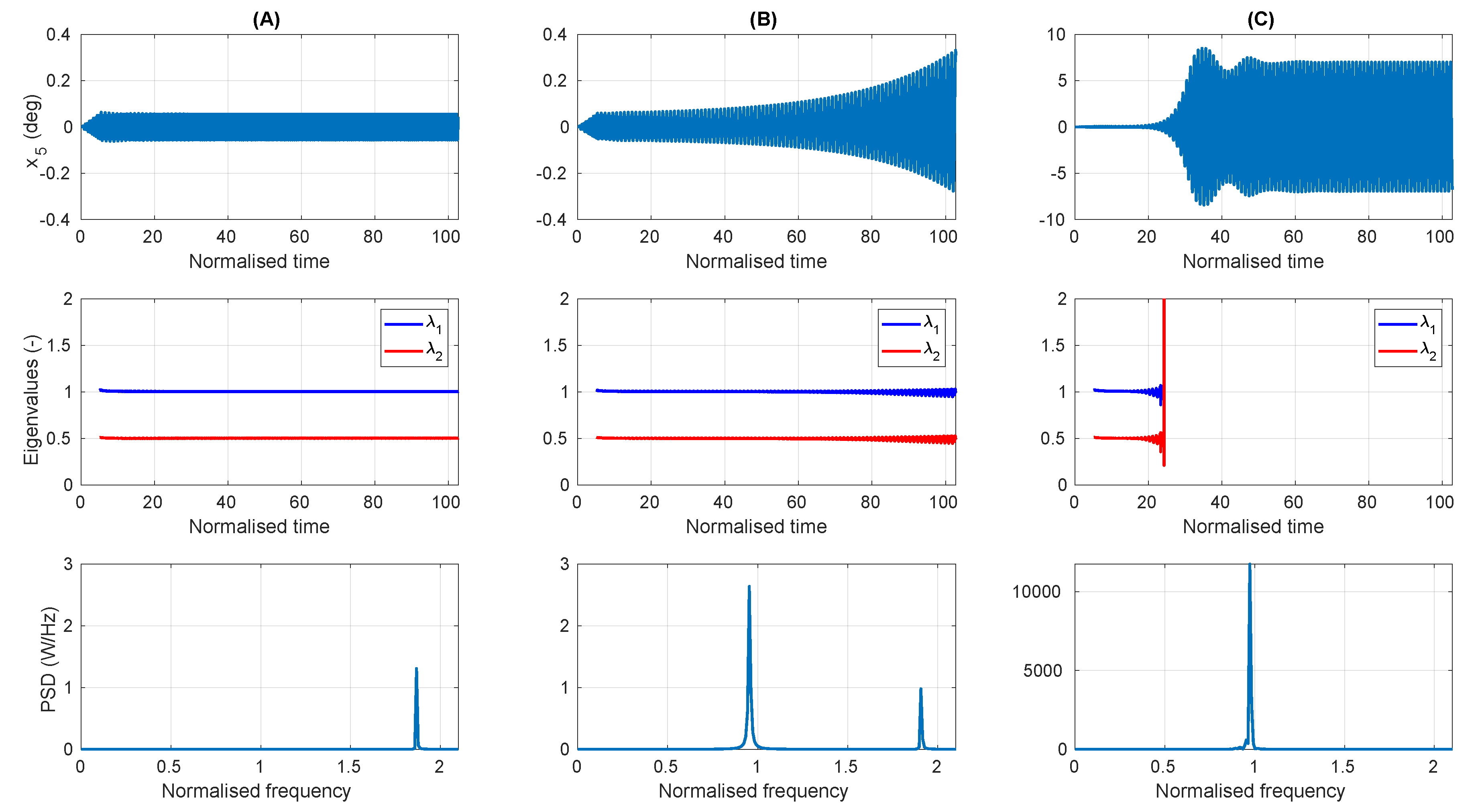
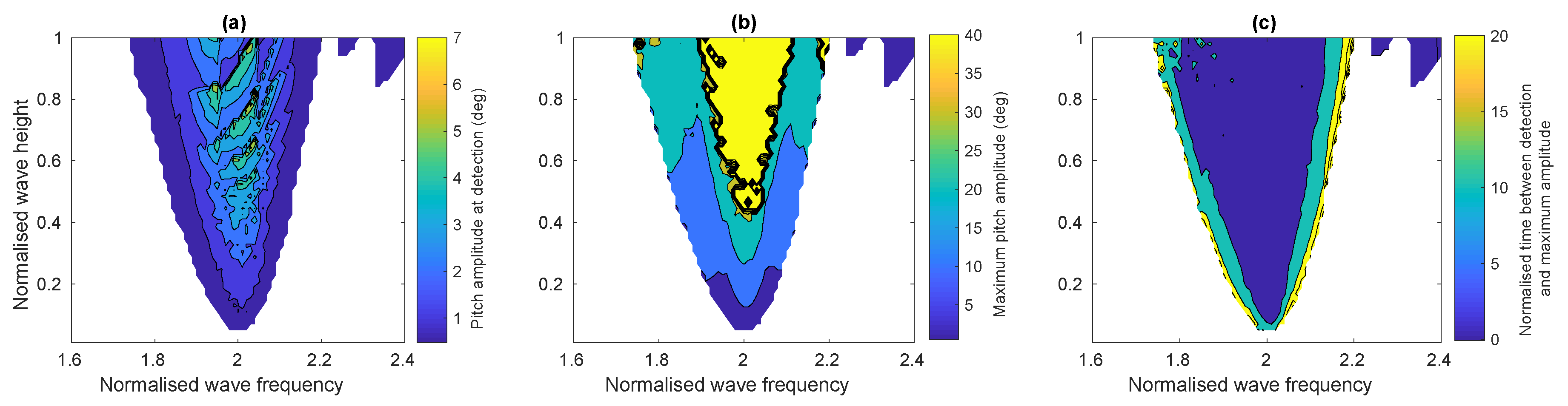
4.1. Monochromatic Waves

To evaluate the performance of the real-time early warning detection system, first each simulation had to be post-processed to determine the instances in which parametric resonance occurred (Section 4.1.1). Once the regions of parametric resonance were identified, then the performance of the early warning detection system could be assessed on its ability to correctly identify the onset of parametric resonance in a timely manner (Section 4.1.2).

4.1.1. Post Process Identification of Parametric Resonance

For normal operating conditions, in monochromatic waves, the frequencies of the pitch motion and the input waves are the same. However, when parametric resonance occurs, the frequency of the pitch motion becomes half of the input wave frequency. Therefore, the occurrence of parametric resonance in monochromatic waves can be easily identified during post processing by comparing the frequency of the pitch motion to the input wave frequency.
For each of the 4050 monochromatic wave simulations, a fast fourier Transform (FFT) was performed on the time series of the pitch displacement. If the peak amplitude of the PSD occurred at a frequency less than 75% of the input wave frequency, then it is clear that parametric resonance occurred for that input wave condition. Figure 4 shows the wave frequencies and amplitudes for which parametric resonance occurs (the white region) and where it does not (the grey region). Three points are marked in red on Figure 4, which are subjected to the same wave height but with different frequencies, such that point A lays in the stable (no parametric resonance) region, point B on the border between the two regions and point C in the parametric resonance region. The pitch displacement time series and the PSD for points A, B and C are plotted in Figure 5A–C respectively. The pitch displacement for point A is seen to remain constant, with a small amplitude below 0.1 degrees and a frequency equal to the input wave frequency. For point B, the amplitude slowly grows throughout the simulation and the frequency has two peaks, one equal to the wave frequency and the other at half the wave frequency. For point C, the pitch displacement is seen to grow exponentially (to a value above 10°) and at a frequency equal to half the wave frequency.

4.1.2. Performance of the Early Warning Detection System
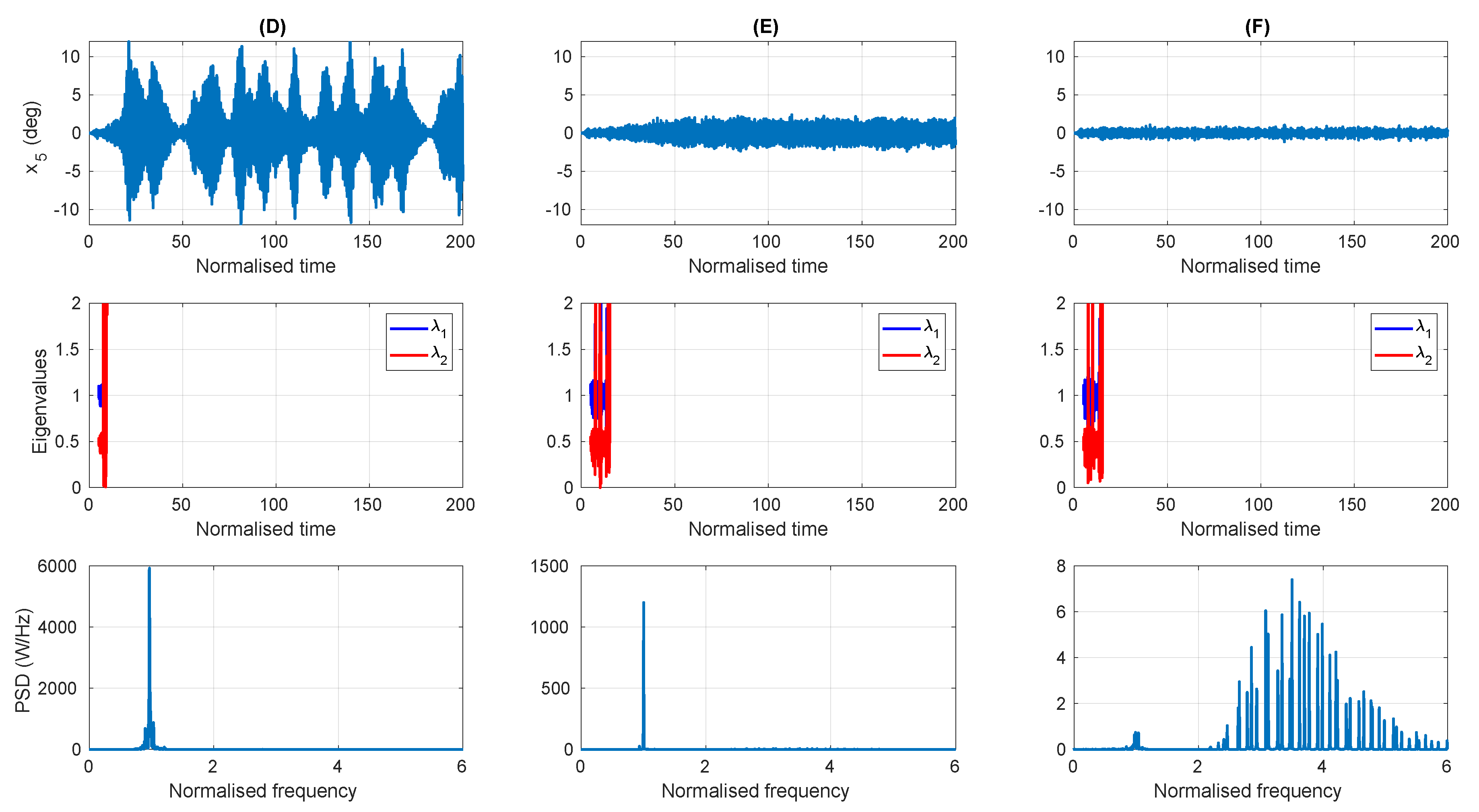
Figure 6 provides the results for the first assessment criteria: correctly warning when parametric resonance occurs (correct positive) and not giving a false warning when parametric resonance does not occur (correct negative). Of the 4050 simulations, the detection system made 4 false negatives and 81 false positives. The false negatives all occurred on the border between the stable and parametric resonance regions, for low wave amplitudes, around twice the pitch natural frequency. The false positives occurred for large wave amplitudes at high frequencies, with three occurring on the border and the remainder occurring in a connected region in the corner of the graph with the highest wave amplitudes and frequencies. The behaviour of the false negatives is explored in Figure 7, which relates to the points A, B and C, marked in red on Figure 6, and the behaviour of the false positives is explored in Figure 8, which relates to the points D, E and F.
Figure 7A relates to point A, which lies outside of the parametric resonance region. The top graph shows the pitch displacement is extremely small, about 0.05°, and the bottom graph shows that the pitch frequency is equal to the input wave frequency, as is expected for normal operating conditions with no parametric resonance. The magnitudes of the eigenvalues, in the middle graph, are seen to remain constant and within the unit circle, signifying that the system is stable. For Figure 7C, since point C lies within the parametric resonance region, the bottom graph shows that the pitch frequency is now equal to half the input wave frequency. The top graph shows that the amplitude of the pitch displacement is approximately 100 times greater than for point A, even though the input wave amplitude is the same for at both points. The magnitudes of the eigenvalues in the middle graph are seen to diverge well outside of the unit complex circle at the same time as the amplitude of the pitch displacement starts to exponentially increase, highlighting the correct performance of the detection system. Since point B is near the border just inside the parametric resonance region, the exponential growth of the pitch displacement, seen in Figure 7B, occurs at a slower rate, only reaching a value of 0.2° by the end of the simulation. The frequency of the pitch displacement has a small peak at the wave frequency, but a larger one at half the wave frequency; thus this simulation is categorised in the parametric resonance region. The magnitudes of the eigenvalues are seen to increase slightly towards the end of the simulation, thus if the simulation ran for a longer time, then the eigenvalues would have likely diverged and the detection system would have correctly identified this case, rather than producing a false negative.
Points D, E and F correspond to the same large input wave amplitude and all trigger the parametric resonance warning system, although point F is a false positive. Figure 8D relates to point D, which is in the top middle of the parametric resonance region, resulting in the pitch motion becoming unstable and exceeding 90° (at which time the simulation is terminated) within approximately 20 wave periods. Figure 8E relates to point E, which is just within the boundary of the parametric resonance region, resulting in large pitch displacements of approximately 30 degrees at half the input wave frequency, which cause the eigenvalues to diverge out of the unit circle. For Figure 8F, which relates to the false positive at point F, the pitch displacement is stable throughout the simulation, with an amplitude less than 0.5° and a frequency equal to the wave frequency. However, although the magnitudes of the eigenvalues do not diverge, the largest eigenvalue has a magnitude of about 2.5, thereby triggering the parametric resonance detection system.
Figure 9a–c highlights the performance of the detection system for the second criteria: how early the system detects the onset of parametric resonance and sends a warning. Figure 9a shows the amplitude of the pitch displacement when the warning system detected parametric resonance, which for the majority of the cases occurred when the pitch displacement was less than 3°. While for some cases, the pitch amplitude was as high as 7° when the warning system detected parametric resonance, these cases correspond to extremely unstable conditions where the pitch displacement diverged within a few periods after the initial ramping of the input wave and exceeded 90° (such as in Figure 8D). The maximum amplitude of the pitch displacement when parametric resonance occurred is shown in Figure 9b1. A quantitative comparison of Figure 9a,b reveals that more that 99% of the detections occurred while the pitch amplitude was less than 1/6 of its maximum amplitude. Finally, Figure 9c shows the normalised time between when the warning system detects the onset of parametric resonance and when the pitch displacement reaches it maximum value. For the majority of cases, the parametric resonance was detected between 5 to 10 T n 5 . For the extremely unstable regions in the top middle of the parametric resonance region, less warning time was available, with the detection occurring between 2 to 5 T n 5 . On the border between the stable and parametric resonance regions, very early warning was given, more than 10 T n 5 , due to the slower exponential growth rate of the pitch displacement amplitude (for example see Figure 8E).

4.2. Polychromatic

In this section, the performance of the real-time early warning detection system is evaluated for polychromatic input waves. Following the same layout as for the monochromatic waves, first each simulation was post-processed to determine the instances in which parametric resonance occurred (Section 4.2.1) and then the performance assessment was conducted (Section 4.2.2).

4.2.1. Post Process Identification of Parametric Resonance

Identifying the occurrence of parametric resonance in polychromatic waves is not as straightforward as for monochromatic waves. For a polychromatic wave spectrum, there is energy in the wave frequencies below the peak of the spectrum; thus, if there is pitch motion at half the peak frequency of the input waves, it can not be instantly identified whether this pitch motion response is due to parametric excitation or direct excitation from the spectral wave components at that lower frequency. Similarly, there is energy at wave frequencies above the peak of the spectrum, so once again it can not be instantly identified whether large pitch motion at low frequencies is due to direct excitation from the wave components at that frequency, or from parametric excitation caused by the wave components at twice that frequency. Therefore, a different metric is applied for the polychromatic waves, based on the energy increase in the pitch motion observed during the simulation.
The energy in the pitch motion (calculated from the root mean square value of x 5 ), measured in the first 5 T n 5 after the input wave height is ramped to maximum amplitude (i.e., from 5 T n 5 to 10 T n 5 ), is compared to the energy in the last 5 T n 5 of the simulation (i.e., from 195 T n 5 to 200 T n 5 ). The energy increase in the pitch motion as a function of the normalised wave frequency and height is shown in the contour plot in Figure 10. The contour lines have a resolution of 0.25 and it can be seen that for low amplitude waves and for frequencies well away from 2 ω n , 5 , the energy is relatively constant over the length of the simulation, with the increase in energy laying between the 0.5 and 1.5 contour lines. However, for the region of larger amplitude waves centred around 2 ω n , 5 , where parametric resonance was expected, the increase in energy has a large positive gradient with respect to the wave height and frequency once the increase in energy values exceeds 1.5. Based on the results shown in Figure 10, if the energy increase from the start to the end of the simulation is more than 2, then the simulation is added to the parametric resonance region, as depicted in Figure 11.
As an example, three points marked in red, A, B and C, were selected, spanning the borderline between the stable and parametric resonance regions; their time series and PSD are plotted in Figure 12. Point A, which is just outside of the parametric resonance region, is seen to have a fairly constant pitch displacement amplitude, whose frequency components are predominantly in a spectrum which has a peak frequency equal to the peak frequency of the input wave spectrum. However, some frequency components exist, centred at half the peak frequency, whose amplitude is about half of the amplitude at the peak frequency. For point B, just inside parametric resonance region, the pitch motion still contains a spectrum of frequency components with a peak frequency equal to the peak frequency of the input wave spectrum and whose amplitudes are approximately the same as for point A. However, the frequency component at half the peak frequency of the input wave spectrum has an amplitude more than 15 times greater than the amplitude at the peak wave frequency. For point C, only the frequency component at half the peak frequency of the input wave spectrum can be seen, whose amplitude is 90 times greater than the amplitude at the peak wave frequency.
To highlight the difference between the classification of normal resonance and parametric resonance, points D, E and F are selected at increasing wave heights on the pitch natural frequency, and their time series and PSD are plotted in Figure 13. The wave height is doubled between points D and E, which results in a doubling of the pitch motion, as is expected for normal resonance. However, between points D and F, the wave height is increased by a factor of three, but the pitch motion increases approximately tenfold, highlighting the nonlinear parametric resonant response.

4.2.2. Performance of the Early Warning Detection System

Figure 14 provides the results for the first assessment criteria: correctly warning when parametric resonance occurs (correct positive) and not giving a false warning when parametric resonance does not occur (correct negative). Of the 2800 simulations, the detection system had 25 false negatives and 235 false positives. The false negatives occurred along the border between the stable and the parametric resonance regions, for low wave amplitudes. The false positives, on the other hand, spanned an area from the border into the stable region, at large wave amplitudes, for both low and high frequencies.
Figure 15A–C shows the time series of the pitch displacement and the magnitudes of the eigenvalues of the matrix A , along with the PSD of the pitch displacement, for points A–C, respectively. While point A corresponds to a false positive and point C corresponds to a false negative, their time series look quite similar. The increase of energy between the start and end of the simulation was 190% for point A and 232% for point B; thus, they both sit very close on either side of the selected threshold for which the parametric resonance region was defined in this study. At the ends of both simulations, large pitch oscillations occurred, with a maximum amplitude of 0.57° for point A, which caused the largest eigenvalue to grow to an absolute value of 264 and trigger the detection system. For point B, the pitch displacement amplitude only grew to 0.48° and the eigenvalues only grew to 1.44. For a comparison to the behaviour of these two points that sit on the borderline, point B sits just inside the parametric resonance region, with the same amplitude as point A and the same frequency as point C, but the energy increased by more than 800% from the start to the end of the simulation, and the maximum pitch displacement was about three times greater than for points A and C.
Yhe false positives at large wave amplitudes, Figure 16D–F, correspond to the points D–F, respectively, which are all subjected to an input spectrum with the same wave height. Point D is well within the parametric resonance region, point E is just inside the parametric resonance region and point F is in the stable region. Point D is seen to have an oscillatory, large amplitude pitch displacement, with rapid exponential growth and decay rates, and a single dominant frequency at half the peak frequency of the input wave spectrum. Point E also has a single dominant frequency at half the peak frequency of the input wave spectrum. However, the maximum amplitude of the pitch displacement is about 20% of the amplitude at point D and grows much slower and remains fairly constant once it reaches its maximum. For point F, the pitch displacement has a much smaller amplitude, which does not grow, and its frequency content is distributed in a spectrum with the same peak as the input waves. However, the magnitudes of the eigenvalues for point F are seen to diverge in much the same way as for points D and E.
Figure 17a–c highlights the performance of the detection system for the second criteria: how early the system detects the onset of parametric resonance and sends a warning. Figure 17a shows that for the majority of the cases, the detection system sends a warning when the pitch displacement amplitude is less than 1 degree, and in all cases before the amplitude reaches 2°. For the polychromatic waves, the maximum pitch amplitude is generally less than 20 degrees, except in a highly unstable region (normalised wave heights above 0.8 and normalised frequencies between 1.25 and 2) where the simulations are terminated at a pitch amplitude of 90°. Near the parametric resonance border and in the region of false positives, the maximum displacement is less than 5°. A quantitative comparison of Figure 17a,b reveals that more that 91% of the detections occurred while the pitch amplitude was less than 1/3 of its maximum amplitude and 67% while the pitch amplitude was less than 1/6 of its maximum amplitude. Finally, Figure 17c shows the normalised time between detection and the maximum amplitude, which is in excess of 10 T n 5 for all cases within the parametric resonance region, and in many cases is more than 100 T n 5 . The reason for the large times is that after the pitch amplitude grows larger, due to parametric resonance, it will then have a degree of variation around the new mean amplitude because of the irregular nature of the input waves. Therefore the maximum amplitude can occur at any time after the initial growth to the larger mean amplitude. For example, in Figure 16E, the pitch amplitude grows to a mean maximum level of about 2° within 60 T n 5 ; however, at 110 T n 5 the amplitude has a spike up to 2.4° which is the maximum value for the simulation.

4.3. Discussion

Overall, the results demonstrate the ability of the proposed system to effectively detect the onset of parametric resonance. The detection occurred in most cases while the pitch oscillations were small fractions of their maximum amplitudes, with many periods of early warning given for a control system to mitigate the impending growth of the pitch oscillations. For the extremely unstable conditions, much less warning time was available; however, these conditions occurred in the middle of the parametric resonance region. Thus, for such waves conditions to develop the sea state must first transition through the wave conditions in the border of the parametric resonance region, where ample warning for the potential instability of the pitch oscillations is provided.
The proposed system rarely failed to detect the occurrence of parametric resonance, with very few false negatives observed, especially for the monochromatic wave case. For the polychromatic wave case, the slightly higher percentage of false negatives might be attributed to the arbitrary classification of the parametric resonance region. As described in Section 4.2.1, if the energy of the pitch oscillations doubled from the start compared to the end of the simulation, then the simulation was classified as belonging to the parametric resonance region. From Figure 10, choosing a 2-fold increase in the energy of the pitch oscillations as the cut-off for the parametric resonance region seems like a reasonable choice, representing the knee of the curve, above which the pitch oscillation amplitude readily increases. However, choosing a slightly larger value around the knee of the curve, such as a 3-fold increase in the energy for example, could also be valid and might have resulted in a lower number of false negatives, but possibly at the cost of an increased number of false positives. Nevertheless, the false negatives produced by the detection system under the current classification system are not particularly troublesome, relating to pitch displacements of less than 1°.
The main advantages of the proposed system relate to its simplicity in terms of computational modelling and required inputs. The detection system does not require a complex, high-fidelity, computationally expensive model. Instead, the simple black-box, linear model in Equation (1) has only four parameters that are adaptively tuned to any type of WEC system/geometry. This allows the detection system to be arbitrarily applied to different type of WECs, without requiring bespoke modelling to be tailored for each individual application, system and/or DoF. Indeed, another advantage of the detection system is its ability to treat each DoF independently, since it updates the parameters of a single DoF model using measurements of that single DoF. Thus, if multiple DoFs are to be considered, each DoF can be treated individually with its own detection system, independent of the other DoFs. However, the system requires that the dynamics of the DoF to be modelled can be approximated by a linear second-order differential equation, which is a reasonable assumption in most cases since the DoFs for which parametric resonance is to be monitored are not the primary mode of motion and amplitudes are relatively small in normal operating conditions. Future work will investigate different types of WECs and DoFs.
Perhaps the biggest advantage is the relatively simple and accessible set of inputs required by the detection system: the position and velocity of a single DoF. Measurement of these variables is relatively straightforward, using accelerometers, inclinometers, etc. However, the robustness of the detection system to noise and error in these measuring instruments should be investigated in future work. Nevertheless, the ability of the detection system to work without requiring more challenging inputs, such as prediction of the input waves or estimation of the excitation force, is a major advantage. The current inputs simplify the system requirements and remove the uncertainty/error involved with prediction and estimation methods.
Being a first implementation, for a real-time detection system for the onset of parametric resonance in WECs, the proposed system is not without its flaws and has room for improvement. The main disadvantage observed from the results was the number of false positives. For the monochromatic waves, the false positives occurred for the high frequency and large amplitude input waves, whereas for the polychromatic waves the false positives occurred for both high and low frequency input waves with large amplitudes.
One possible remedy to reduce the amount of false positives is to increase the detection threshold, i.e., the value of ϵ in Equation (19). For example, as seen in Figure 8F, increasing the value of ϵ from 1 to 3 would eliminate the false positive. Although increasing the detection threshold can in theory increase the number of false negatives, in practice when parametric resonance was detected the magnitudes of the eigenvalues typically diverged very rapidly to values exceeding 1000. For many false positives, the magnitudes of the eigenvalues were less than 10. Thus, it is unlikely that increasing the detection threshold to any single digit number would cause a currently correct positive detection to become a false negative. However, a false negative is more detrimental to the WEC system than a false positive, so prudently selecting the value of ϵ should be investigated on a case-by-case basis for different WEC systems and DoFs.
Alternatively, to reduce the nuumber of false positives, the underlying cause should be identified if possible and the detection algorithm improved accordingly. In particular, a possible explanation for the growth of the eigenvalues, which trigger the false detection, is due to the input excitation not being Gaussian white noise, as is assumed in Equation (1). The Gaussian white noise assumption stems from the original application of this detection method in [51], the roll motion of ships, for which in head seas there is no direct wave excitation to the roll DoF. In contrast, the present case study examined the pitch motion, which is directly excited by the input waves. Both the monochromatic and polychromatic waves were coloured, rather than a white spectrum; thus the assumption of a Gaussian white noise excitation was violated since the input spectrum was not flat, with equal amplitude across all frequencies. Therefore, future work will investigate a means to improve upon the assumption of Gaussian white noise input whilst hopefully maintaining the benefit of not explicitly requiring an estimation of the input waves/excitation force.

5. Conclusions

This paper demonstrated the first implementation of a real-time detection system for the early warning of the onset of parametric resonance in a WEC, by applying a method developed for the monitoring and detection of parametric roll motion in ships. The results from a test case, considering the parametric pitch motion in a heaving spar-buoy, show that the detection system performed very well, achieving 95% accuracy across a range of monochromatic and polychromatic sea states. In addition, the detection system provides an early warning while the pitch motion is a small fraction of its impending maximum amplitude. However, one potential shortcoming is the assumption of the external excitation to the system being described by Gaussian white noise, which is less valid for the pitch motion in a WEC compared to the roll motion in a ship. Assuming the input to be Gaussian white noise resulted in the system incorrectly detecting instability when the input waves were of large amplitudes and high frequencies, resulting in the warning system providing 10 times more false positives than false negatives. The practical implementation of the system imposes a low overhead, only requiring measurement of the position and velocity of the DoF to be monitored and enough computational resources to perform a recursive least squares algorithm for two time-varying parameters and then finding the roots of a quadratic equation.

Author Contributions

Conceptualization, J.D.; Formal analysis, J.D.; Investigation, J.D.; Supervision, T.K.-N.; Writing—original draft, J.D.; Writing—review & editing, T.K.-N. All authors have read and agreed to the published version of the manuscript.

Funding

This project has received funding from the European Union’s Horizon 2020 research and innovation programme under the Marie Sklodowska-Curie grant agreement number 867453. The research reported in this paper was supported by the BME Water Sciences and Disaster Prevention TKP2020 IE grant of NKFIH Hungary (BME IE-VIZ TKP2020) and by the BME NC TKP2020 grant of NKFIH Hungary.

Conflicts of Interest

The authors declare no conflict of interest.

References

  1. Fossen, T.; Nijmeijer, H. Parametric Resonance in Dynamical Systems; Springer: New York, NY, USA, 2011. [Google Scholar]
  2. Faraday, M. On a peculiar class of acoustical figures; and on certain forms assumed by groups of particles upon vibrating elastic surfaces. In Philosophical Transactions of the Royal Society of London; The Royal Society: London, UK, 1831; pp. 299–340. [Google Scholar]
  3. Froude, W. On the Rolling of Ships; Institution of Naval Architects: London, UK, 1861. [Google Scholar]
  4. Galeazzi, R. Autonomous Supervision and Control of Parametric Roll Resonance. Ph.D. Thesis, Department of Naval Architecture and Offshore Engineering, Technical University of Denmark, Lyngby, Denmark, 2009. [Google Scholar]
  5. Shigunov, V.; El Moctar, O.; Rathje, H.; Germanischer Lloyd, A. Conditions of parametric rolling. In Proceedings of the 10th International Conference on Stability of Ships and Ocean Vehicles, St Petersberg, Russia, 22–26 June 2009. [Google Scholar]
  6. Koo, B.; Kim, M.; Randall, R. Mathieu instability of a spar platform with mooring and risers. Ocean Eng. 2004, 31, 2175–2208. [Google Scholar] [CrossRef]
  7. Neves, M.A.; Sphaier, S.H.; Mattoso, B.M.; Rodri´ guez, C.A.; Santos, A.L.; Vileti, V.L.; Torres, F.G. On the occurrence of Mathieu instabilities of vertical cylinders. In Proceedings of the 27th International Conference on Offshore Mechanics and Arctic Engineering, Estorill, Portugal, 15–20 June 2008. [Google Scholar]
  8. Li, B.B.; Ou, J.P.; Teng, B. Numerical investigation of damping effects on coupled heave and pitch motion of an innovative deep draft multi-spar. J. Mar. Sci. Technol. 2011, 19, 231–244. [Google Scholar]
  9. Yang, H.; Xu, P. Effect of hull geometry on parametric resonances of spar in irregular waves. Ocean Eng. 2015, 99, 14–22. [Google Scholar] [CrossRef]
  10. Jang, H.; Kim, M. Mathieu instability of Arctic Spar by nonlinear time-domain simulations. Ocean Eng. 2019, 176, 31–45. [Google Scholar] [CrossRef]
  11. Umeda, N.; Hashimoto, H.; Minegaki, S.; Matsuda, A. An investigation of different methods for the prevention of parametric rolling. J. Mar. Sci. Technol. 2008, 13, 16–23. [Google Scholar] [CrossRef]
  12. Galeazzi, R.; Pettersen, K.Y. Parametric Resonance in Dynamical Systems; Chapter Controlling Parametric Resonance: Induction and Stabilization of Unstable Motions; Fossen, T.I., Nijmeijer, H., Eds.; Springer: New York, NY, USA, 2012; pp. 305–327. [Google Scholar]
  13. Bracewell, R.H. Frog and PS Frog: A Study of Two Reactionless Ocean Wave Energy Converters. Ph.D. Thesis, University of Lancaster, Lancashire, UK, 1990. [Google Scholar]
  14. Durand, M.; Babarit, A.; Pettinotti, B.; Quillard, O.; Toularastel, J.; Clément, A. Experimental validation of the performances of the SEAREV wave energy converter with real time latching control. In Proceedings of the 7th European Wave and Tidal Energy Conference, Porto, Portugal, 11–13 September 2007. [Google Scholar]
  15. Payne, G.S.; Taylor, J.R.; Bruce, T.; Parkin, P. Assessment of boundary-element method for modelling a free-floating sloped wave energy device. Part 2: Experimental validation. Ocean Eng. 2008, 35, 342–357. [Google Scholar] [CrossRef] [Green Version]
  16. Raftery, M.W. Harnessing Ocean Surface Wave Energy to Generate Electricity. Master’s Thesis, Stevens Institute of Technology, Hoboken, NJ, USA, 2008. [Google Scholar]
  17. Sheng, W.; Flannery, B.; Lewis, A.; Alcorn, R. Experimental studies of a floating cylindrical OWC WEC. In Proceedings of the 31st International Conference on Ocean, Offshore and Arctic Engineering, Rio de Janeiro, Brazil, 1–6 July 2012. [Google Scholar]
  18. Gomes, R.; Henriques, J.; Gato, L.; Falcao, A. Testing of a small-scale floating OWC model in a wave flume. In Proceedings of the 4th International Conference on Ocean Energy, Dublin, Ireland, 17–19 October 2012. [Google Scholar]
  19. Gomes, R.; Henriques, J.; Gato, L.; Falcão, A.d.O. Wave channel tests of a slack-moored floating oscillating water column in regular waves. In Proceedings of the 11th European Wave and Tidal Energy Conference, Nantes, France, 6–11 September 2015. [Google Scholar]
  20. Beatty, S.J.; Roy, A.; Bubbar, K.; Ortiz, J.; Buckham, B.J.; Wild, P.; Stienke, D.; Nicoll, R. Experimental and numerical simulations of moored self-reacting point absorber wave energy converters. In Proceedings of the 25th International Ocean and Polar Engineering Conference, Kona, HI, USA, 25–30 June 2015. [Google Scholar]
  21. Orszaghova, J.; Wolgamot, H.; Taylor, R.E.; Draper, S.; Rafiee, A.; Taylor, P. Simplified dynamics of a moored submerged buoy. In Proceedings of the 32nd International Workshop on Water Waves and Floating Bodies, Dalian, China, 23–26 April 2017. [Google Scholar]
  22. Sergiienko, N.Y. Three-Tether Wave Energy Converter: Hydrodynamic Modelling, Performance Assessment and Control. Ph.D. Thesis, University Adelaide, Adelaide, Australia, 2018. [Google Scholar]
  23. Gomes, R.; Henriques, J.; Gato, L.; Falcão, A. Experimental Tests of a 1: 16th-Scale Model of the Spar-Buoy OWC in a Large Scale Wave Flume in Regular Waves. In Proceedings of the 37th International Conference on Ocean, Offshore and Arctic Engineering, Madrid, Spain, 17–22 June 2018. [Google Scholar]
  24. Kurniawan, A.; Grassow, M.; Ferri, F. Numerical modelling and wave tank testing of a self-reacting two-body wave energy device. Ships Offshore Struct. 2019, 14, 344–356. [Google Scholar] [CrossRef]
  25. Orszaghova, J.; Wolgamot, H.; Draper, S.; Eatock Taylor, R.; Taylor, P.; Rafiee, A. Transverse motion instability of a submerged moored buoy. Proc. R. Soc. A 2019, 475, 20180459. [Google Scholar] [CrossRef] [Green Version]
  26. Gomes, R.; Henriques, J.; Gato, L.; Falcão, A. Time-domain simulation of a slack-moored floating oscillating water column and validation with physical model tests. Renew. Energy 2020, 149, 165–180. [Google Scholar] [CrossRef]
  27. Davidson, J.; Costello, R. Efficient Nonlinear Hydrodynamic Models for Wave Energy Converter Design—A Scoping Study. J. Mar. Sci. Eng. 2020, 8, 35. [Google Scholar] [CrossRef] [Green Version]
  28. Babarit, A.; Mouslim, H.; Clément, A.; Laporte-Weywada, P. On the numerical modelling of the nonlinear behaviour of a wave energy converter. In Proceedings of the 28th International Conference on Offshore Mechanics & Arctic Engineering, Honolulu, HI, USA, 31 May–5 June 2009. [Google Scholar]
  29. Tarrant, K.R. Numerical Modelling of Parametric Resonance of a Heaving Point Absorber Wave Energy Converter. Ph.D. Thesis, Trinity College Dublin, Dublin, Ireland, 2015. [Google Scholar]
  30. Tarrant, K.; Meskell, C. Investigation on parametrically excited motions of point absorbers in regular waves. Ocean Eng. 2016, 111, 67–81. [Google Scholar] [CrossRef]
  31. Giorgi, G.; Ringwood, J.V. A compact 6-DoF nonlinear wave energy device model for power assessment and control investigations. IEEE Trans. Sustain. Energy 2018, 10, 119–126. [Google Scholar] [CrossRef] [Green Version]
  32. Giorgi, G.; Ringwood, J.V. Articulating Parametric Nonlinearities in Computationally Efficient Hydrodynamic Models. IFAC-PapersOnLine 2018, 51, 56–61. [Google Scholar] [CrossRef]
  33. Giorgi, G.; Ringwood, J.V. Parametric motion detection for an oscillating water column spar buoy. In Proceedings of the 3rd International Conference on Renewable Energies Offshore, Lisbon, Portugal, 8–10 October 2018. [Google Scholar]
  34. Giorgi, G.; Gomes, R.P.; Bracco, G.; Mattiazzo, G. The Effect of Mooring Line Parameters in Inducing Parametric Resonance on the Spar-Buoy Oscillating Water Column Wave Energy Converter. J. Mar. Sci. Eng. 2020, 8, 29. [Google Scholar] [CrossRef] [Green Version]
  35. Zou, S.; Abdelkhalik, O.; Robinett, R.; Korde, U.; Bacelli, G.; Wilson, D.; Coe, R. Model Predictive Control of parametric excited pitch-surge modes in wave energy converters. Int. J. Mar. Energy 2017, 19, 32–46. [Google Scholar] [CrossRef] [Green Version]
  36. Yerrapragada, K.; Ansari, M.; Karami, M.A. Enhancing power generation of floating wave power generators by utilization of nonlinear roll-pitch coupling. Smart Mater. Struct. 2017, 26, 094003. [Google Scholar] [CrossRef]
  37. Abdelkhalik, O.; Zou, S. Time-varying linear quadratic gaussian optimal control for three-degree-of-freedom wave energy converters. In Proceedings of the 12th European Wave and Tidal Energy Conference, Cork, Ireland, 27 August–2 September 2017. [Google Scholar]
  38. Abdelkhalik, O.; Zou, S.; Robinett, R.; Bacelli, G.; Wilson, D.; Coe, R. Control of three degrees-of-freedom wave energy converters using pseudo-spectral methods. J. Dyn. Syst. Meas. Control 2018, 140, 074501. [Google Scholar] [CrossRef]
  39. Davidson, J.; Karimov, M.; Szelechman, A.; Windt, C.; Ringwood, J. Dynamic mesh motion in OpenFOAM for wave energy converter simulation. In Proceedings of the 14th OpenFOAM Workshop, Duisburg, Germany, 23–26 July 2019. [Google Scholar]
  40. Zou, S.; Abdelkhalik, O. Time-varying linear quadratic Gaussian optimal control for three-degree-of-freedom wave energy converters. Renew. Energy 2020, 149, 217–225. [Google Scholar] [CrossRef]
  41. Palm, J.; Bergdahl, L.; Eskilsson, C. Parametric excitation of moored wave energy converters using viscous and non-viscous CFD simulations. In Advances in Renewable Energies Offshore; Taylor & Francis Group: Abingdon, UK, 2019; pp. 455–462. [Google Scholar]
  42. Nicoll, R.S.; Wood, C.F.; Roy, A.R. Comparison of physical model tests with a time domain simulation model of a wave energy converter. In Proceedings of the 31st International Conference on Ocean, Offshore and Arctic Engineering, Rio de Janeiro, Brazil, 1–6 July 2012. [Google Scholar]
  43. Orszaghova, J.; Wolgamot, H.; Draper, S.; Taylor, P.H.; Rafiee, A. Onset and limiting amplitude of yaw instability of a submerged three-tethered buoy. Proc. R. Soc. A 2020, 476, 20190762. [Google Scholar] [CrossRef]
  44. Rho, J.B.; Choi, H.S.; Shin, H.S.; Park, I.K. A study on Mathieu-type instability of conventional spar platform in regular waves. Int. J. Offshore Polar Eng. 2005, 15, 104–108. [Google Scholar]
  45. Ortiz, J.P. The Influence of Mooring Dynamics on the Performance of Self Reacting Point Absorbers. Master’s Thesis, University of Victoria, Victoria, BC, Canada, 2016. [Google Scholar]
  46. Gomes, R.; Malvar Ferreira, J.; Ribeiro e Silva, S.; Henriques, J.; Gato, L. An experimental study on the reduction of the dynamic instability in the oscillating water column spar buoy. In Proceedings of the 12th European Wave and Tidal Energy Conference, Cork, Ireland, 27 August–2 September 2017. [Google Scholar]
  47. Cordonnier, J.; Gorintin, F.; De Cagny, A.; Clément, A.; Babarit, A. SEAREV: Case study of the development of a wave energy converter. Renew. Energy 2015, 80, 40–52. [Google Scholar] [CrossRef]
  48. Gomes, R.; Henriques, J.; Gato, L.; Falcao, A. An upgraded model for the design of spar-type floating oscillating water column devices. In Proceedings of the 13th European Wave and Tidal Energy Conference, Naples, Italy, 1–6 September 2019. [Google Scholar]
  49. Villegas, C.; van der Schaaf, H. Implementation of a pitch stability control for a wave energy converter. In Proceedings of the 10th European Wave and Tidal Energy Conference, Southampton, UK, 5–9 September 2011. [Google Scholar]
  50. Maloney, P. Performance Assessment of a 3-Body Self-Reacting Point Absorber Type Wave Energy Converter. Master’s Thesis, University of Victoria, Victoria, BC, Canada, 2019. [Google Scholar]
  51. Holden, C.; Perez, T.; Fossen, T.I. Frequency-motivated observer design for the prediction of parametric roll resonance. IFAC Proc. Vol. 2007, 40, 57–62. [Google Scholar] [CrossRef]
  52. Shaw McCue, L.; Bulian, G. A numerical feasibility study of a parametric roll advance warning system. J. Offshore Mech. Arct. Eng. 2007, 129. [Google Scholar] [CrossRef]
  53. Galeazzi, R.; Blanke, M.; Poulsen, N.K. Parametric roll resonance detection on ships from nonlinear energy flow indicator. IFAC Proc. Vol. 2009, 42, 348–353. [Google Scholar] [CrossRef]
  54. Galeazzi, R.; Blanke, M.; Poulsen, N.K. Early detection of parametric roll resonance on container ships. IEEE Trans. Control Syst. Technol. 2012, 21, 489–503. [Google Scholar] [CrossRef] [Green Version]
  55. Galeazzi, R.; Blanke, M.; Falkenberg, T.; Poulsen, N.K.; Violaris, N.; Storhaug, G.; Huss, M. Parametric roll resonance monitoring using signal-based detection. Ocean Eng. 2015, 109, 355–371. [Google Scholar] [CrossRef] [Green Version]
  56. Caamaño, L.S.; González, M.M.; Casás, V.D. On the feasibility of a real time stability assessment for fishing vessels. Ocean Eng. 2018, 159, 76–87. [Google Scholar] [CrossRef]
  57. Caamaño, L.S.; Galeazzi, R.; Nielsen, U.D.; González, M.M.; Casás, V.D. Real-time detection of transverse stability changes in fishing vessels. Ocean Eng. 2019, 189, 106369. [Google Scholar] [CrossRef]
  58. Davidson, J.; Genest, R.; Ringwood, J. Adaptive control of a wave energy converter simulated in a numerical wave tank. In Proceedings of the 12th European Wave and Tidal Energy Conference, Cork, Ireland, 27 August–2 September 2017. [Google Scholar]
  59. Genest, R.; Davidson, J.; Ringwood, J.V. Adaptive control of a wave energy converter. IEEE Trans. Sustain. Energy 2018, 9, 1588–1595. [Google Scholar]
  60. Peña-Sanchez, Y.; Windt, C.; Davidson, J.; Ringwood, J.V. A Critical Comparison of Excitation Force Estimators for Wave-Energy Devices. IEEE Trans. Control. Syst. Technol. 2019. [Google Scholar] [CrossRef]
  61. Thompson, J.M.T.; Stewart, H.B. Nonlinear Dynamics and Chaos; John Wiley & Sons: Hoboken, NJ, USA, 2002. [Google Scholar]
  62. Yong-Pyo, H.; Dong-Yeon, L.; Yong-Ho, C.; Sam-Kwon, H.; Se-Eun, K. An experimental study on the extreme motion responses of a spar platform in the heave resonant waves. In Proceedings of the 15th International Offshore and Polar Engineering Conference, Seol, Korea, 19–24 June 2005. [Google Scholar]
  63. Zhao, J.; Tang, Y.; Shen, W. A study on the combination resonance response of a classic spar platform. J. Vib. Control 2010, 16, 2083–2107. [Google Scholar] [CrossRef]
  64. Gavassoni, E.; Gonçalves, P.B.; Roehl, D.M. Nonlinear vibration modes and instability of a conceptual model of a spar platform. Nonlinear Dyn. 2014, 76, 809–826. [Google Scholar] [CrossRef]
  65. Giorgi, G.; Davidson, J.; Habib, G.; Bracco, G.; Mattiazzo, G.; Kalmar-Nagy, T. Nonlinear Dynamic and Kinematic Model of a Spar-Buoy: Parametric Resonance and Yaw Numerical Instability. Mar. Sci. Eng. 2020, 8, 504. [Google Scholar] [CrossRef]
  66. Wacher, A.; Nielsen, K. Mathematical and numerical modeling of the AquaBuOY wave energy converter. Math. Case Stud. 2010, 2, 16–33. [Google Scholar]
1.
Note: to limit the scale, the maximum amplitude is clipped at 40°, since for any simulation in which the amplitude exceeded this value, the pitch displacement grew to 90° and the simulation was terminated.
Figure 1. Example of the input waves: (a) monochromatic, (b) polychromatic, (c) power spectral density (PSD) of the polychomatic waves.
Jmse 08 00819 g001
Figure 2. The excitation force coefficients (a) H E , 3 , (b) ϕ E , 3 , (c) H E , 5 and (d) ϕ E , 5 .
Jmse 08 00819 g002
Figure 3. The online adaptation of θ i , k using the recursive least squares algorithm. For monochromatic waves with: (a) a normalised wave frequency of 1.6 and varying wave height; (b) a normalised wave amplitude of 0.01 and varying wave frequency; and (c) a normalised wave frequency of 3, a normalised wave height of 0.1 and varying initial values.
Jmse 08 00819 g003
Figure 4. The amplitude and frequency range spanned by the monochromatic waves test cases. The white region denotes where parametric resonance was observed. Note the inclusion of grid lines in this figure to highlight the frequency and amplitude resolution, with a result simulated at every grid intersection. For reference, as discussed in Section 3.1, the wave height is normalised against G M ¯ and the wave frequency by ω n , 5 .
Jmse 08 00819 g004
Figure 5. The pitch displacement time series and resulting PSD for the points (A) A, (B) B and (C) C in Figure 4.
Jmse 08 00819 g005
Figure 6. The performance of the early warning detection system in monochromatic waves; correct positives (white), correct negatives (grey), false positives (dark grey) and false negatives (black).
Jmse 08 00819 g006
Figure 7. The pitch displacement time series (top), the magnitudes of the eigenvalues of the matrix A (middle) and the PSD of the pitch displacement (bottom), for the points (A) A, (B) B and (C) C in Figure 6.
Jmse 08 00819 g007
Figure 8. The pitch displacement time series (top), the magnitudes of the eigenvalues of the matrix A (middle) and the PSD of the pitch displacement (bottom), for the points (D) D, (E) E and (F) F in Figure 6.
Jmse 08 00819 g008
Figure 9. The performance of the early warning detection system in monochromatic waves. (a) The amplitude of the pitch displacement when the warning system detected parametric resonance. (b) The maximum amplitude of the pitch displacement when parametric resonance occurred (clipped at 40°, above which simulations always crashed). (c) The time between the when the warning system detected parametric resonance and when the maximum pitch displacement occurred.
Jmse 08 00819 g009
Figure 10. The energy increase in the pitch displacement from the start to the end of the simulation as a function of the normalised wave frequency and height. The contour lines have a resolution of 0.25.
Jmse 08 00819 g010
Figure 11. The amplitude and frequency range spanned by the polychromatic waves’ test cases. The region in which parametric resonance was observed is shown in white.
Jmse 08 00819 g011
Figure 12. The pitch displacement time series and resulting PSD for the points (A) A, (B) B and (C) C in Figure 11.
Jmse 08 00819 g012
Figure 13. The pitch displacement time series and resulting PSD for the points (D) D, (E) E and (F) F in Figure 11.
Jmse 08 00819 g013
Figure 14. The performance of the early warning detection system in polychromatic waves; correct positives (white), correct negatives (grey), false positives (dark grey) and false negatives (black).
Jmse 08 00819 g014
Figure 15. The time series for the pitch displacement (top), the magnitudes of the eigenvalues of the matrix A (middle) and the PSD of the pitch displacement (bottom), for the points (A) A, (B) B and (C) C in Figure 14.
Jmse 08 00819 g015
Figure 16. The time series for the pitch displacement (top), the magnitudes of the eigenvalues of the matrix A (middle) and the PSD of the pitch displacement (bottom), for the points (D) D, (E) E and (F) F in Figure 14.
Jmse 08 00819 g016
Figure 17. The performance of the early warning detection system in polychromatic waves. (a) The amplitude of the pitch displacement when the warning system detected parametric resonance. (b) The maximum amplitude of the pitch displacement when parametric resonance occurred (clipped at 40°, above which simulations always crashed). (c) The time between the when the warning system detected parametric resonance and when the maximum pitch displacement occurred.
Jmse 08 00819 g017
Table 1. Model parameter values used in the test case.
ParameterValueParameterValueParameterValue
A C 1087 m2 ρ 1000 kg/m3M2.15 × 108 kg
L D 198.1 mg9.81 m/s2 m 3 1.37 × 10 7 kg
G M ¯ 10.1 m C 3 1.19 × 10 6 kg/s I 5 1.12 × 10 12 kgm
L M S 109.1 m C 5 7.54 × 10 9 kgm/s m 5 7.26 × 10 11 kg
Publisher’s Note: MDPI stays neutral with regard to jurisdictional claims in published maps and institutional affiliations.

