Simple Controllers for Wave Energy Devices Compared

Abstract

The design of controllers for wave energy devices has evolved from early monochromatic impedance-matching methods to complex numerical algorithms that can handle panchromatic seas, constraints, and nonlinearity. However, the potential high performance of such numerical controller comes at a computational cost, with some algorithms struggling to implement in real-time, and issues surround convergence of numerical optimisers. Within the broader area of control engineering, practitioners have always displayed a fondness for simple and intuitive controllers, as evidenced by the continued popularity of the ubiquitous PID controller. Recently, a number of energy-maximising wave energy controllers have been developed based on relatively simple strategies, stemming from the fundamentals behind impedance-matching. This paper documents this set of (5) controllers, which have been developed over the period 2010–2020, and compares and contrasts their characteristics, in terms of energy-maximising performance, the handling of physical constraints, and computational complexity. The comparison is carried out both analytically and numerically, including a detailed case study, when considering a state-of-the-art CorPower-like device.

1. Introduction

Despite being a vast resource, wave energy conversion technology has not yet reached economic commercialisation. The main reason for the lack of proliferation of wave energy can be attributed to the fact that harnessing the irregular reciprocating motion of the sea is not as straightforward as, for example, extracting energy from the wind. This is clearly reflected in the striking absence of clear technology convergence, with over a thousand different concepts and patents proposed over the years (see, for instance, [1]).

Dynamic analysis and control system technology can impact many aspects of wave energy converter (WEC) design and operation, including device sizing and configuration, maximising energy extraction from waves, and optimising energy conversion in the power take-off (PTO) system. As a matter of fact, it is already clear (and well-established) that appropriate control technology has the capability to greatly enhance energy extraction from WECs [2,3]. In particular, the control input, supplied by means of the PTO system, and effectively realising the mechanical load on the device, plays a key role in the optimisation of the operation of wave energy devices: Ultimately, energy conversion must be performed as economically as possible, to minimise the delivered energy cost, while also maintaining the structural integrity of the device, minimising wear on WEC components, and operating across a wide range of sea conditions. This is virtually always written in terms of an energy-maximising criterion, so that the control problem for WECs can be informally posed [2] as depicted in

Table 1. Control problem for WECs.

Design the PTO Force (Control Input) Such That:
Maximises	Energy absorption from incoming waves.
Subject to	WEC dynamics.
	Device and actuator physical limitations.

:

In recent years, wave energy control researchers applied optimal control methods, where the energy-maximisation design is written in terms of an appropriate optimal control problem (OCP), and well-developed techniques (mainly originated within the theory of calculus of variations [4]) can be considered. In particular, direct optimal control techniques are often adopted [5], which discretise the variables involved in the WEC OCP, and attempt to maximise the resulting nonlinear program (NP) directly. This NP has to be solved while using numerical optimisation routines, whose complexity (both analytical and computational) depends upon a number of factors, including the specific discretisation method selected. This family of optimisation-based controllers is optimal by design, facilitated by a suitable definition of the energy-maximising control objective in the corresponding OCP. In addition, device safety can be directly addressed by adding a (feasible) set of constraints (i.e., device and actuator limitations) to the optimisation problem.

Although optimal by design, these optimisation-based controllers have their specific drawbacks, which can limit their application in ‘real-world’ scenarios. In particular, depending on the discretisation utilised, optimisation-based controllers may or may not be suitable for real-time implementation; the complexity of the associated NP, and the numerical routines that are required to approximate its solution, can preclude real-time operation, often especially true if nonlinearities are considered in the WEC dynamical model [6]. In addition, these controllers often lack of any ‘intuitive’ interpretation, given the mathematical complexity behind their derivation. In other words, very specific expertise is often required to design, synthesise, and calibrate these controllers, which is relatively unappealing for industrial practitioners.

Aiming to find simple and intuitive solutions, a number of researchers attempt to solve the WEC OCP while using fundamental theory behind maximum power transfer: the so-called impedance-matching principle [7]. In particular, this family of simple controllers attempts to provide a (physically implementable) realisation of the impedance-matching condition for maximum power transfer, by proposing simple systems, mostly characterised by well-known techniques from linear time-invariant theory. These techniques have mild computational requirements, and their implementation can be performed in real-time with almost any physical hardware platform, including commercial low-cost microcontrollers.

Naturally, this simplicity comes at a certain cost: altough simple to implement, the performance of these controllers is inherently suboptimal, leading to a drop in energy absorption when compared to optimisation-based techniques. In addition, and since the impedance-matching condition does not consider any physical limitations (i.e., device and actuator limits), constraint handling is virtually always performed by means of simple mechanisms, which do not take into account optimality with respect to power absorption. In other words, the limitation mechanisms are designed independently from the energy-maximising objective, effectively providing constrained optimal solutions, rather than optimal constrained solutions. This naturally implies a loss of energy absorption under constrained conditions.

Nonetheless, despite their suboptimal performance, the main advantage of these controllers relies on their simplicity of implementation, and intuitive design, synthesis, and calibration, which makes this family of strategies highly appealing for practical applications. Additionally, it is worth noting that, when considering the simplicity of controllers based on the impedance-matching principle, this family of controllers can be implemented in almost any physical hardware platform, such as commercial low cost microcontrollers while using traditional discrete-time recursive routines, which represents one of the main features of these controllers. Motivated by the potential that is offered by this set of techniques in real-world scenarios, this paper documents a critical comparison between five (5) different controllers, developed over the period 2010–2020. It is important to note that, even though the origins of impedance-matching control originate in the 1970s [8], practical algorithms dealing with panchromatic operation and system constraints were only developed within the past decade, hence the focus on the period post 2010’. In particular, this study compares and contrasts their characteristics, in terms of energy-maximising performance, the handling of physical constraints, and computational load. The comparison is carried out both analytically and numerically, with special attention paid to the stability issue that can arise in the implementation of each selected strategy. These controllers are those published in [9,10,11,12,13], listed, in chronological order, in

Table 2. Set of five (5) simple controllers compared in this study.

Reference	Controller Name	Shorthand Notation
[9]	Suboptimal causal reactive controller	C1
[10]	Simple and effective real-time controller	C2
[11]	Multi resonant feedback controller	C3
[12]	Feedback resonating controller	C4
[13]	LiTe-Con	C5

.

Note that, in Table 2, the column ‘Controller name’, is defined while using the title of each corresponding reference. It should be noted that, in terms of operation and performance of this set of controller under real conditions in open waters, the control algorithms reviewed in this paper are designed to operate only in the power production region of sea states and devices; under extreme wave conditions, a supervisory control system will put the system into a safe configuration, under which no power is produced.

The remainder of this paper is organised as follows. Section 1.1 introduces the mathematical notation used throughout this study. Section 2 presents the fundamentals behind control-oriented modelling of WECs, while Section 3 provides a detailed description of the fundamental principle of impedance-matching, highlighting each of its features. Section 4 outlines the theory behind the design and synthesis of each of the five (5) simple controllers that are listed in Table 2, in chronological order of publication. Section 5 presents a case study based on a full-scale CorPower-like device, where the set of selected simple controllers is assessed in terms of a number of indicators, including energy-maximising performance, constraint handling, computational complexity, and stability features. Section 6 provides a detailed discussion on the results that are presented in Section 5, specifically providing insight into each of the strenghts and weaknesses of each simple controller. Finally, Section 7 encompasses the main conclusions of this study.

1.1. Notation

Standard notation is considered throughout this paper, most of which is defined in this section. ${\mathbb{R}}^{+}$ (${\mathbb{R}}^{-}$) denotes-* the set of non-negative (non-positive) real numbers. The notation ${\mathbb{N}}_q$ indicates the set of all positive natural numbers up to q, i.e., ${\mathbb{N}}_q=\{1,2,\cdots ,q\}$. The symbol 0 stands for any zero element, dimensioned according to the context. The notation $A^{🟉}$, with $A\in {\mathbb{C}}^{n\times n}$, denote the Hermitian transpose of the matrix A. The notation $\mathbb{R}\mathrm{𝕖}\left\{z\right\}$ and $\mathbb{Im}\left\{z\right\}$, with $z\in \mathbb{C}$, stands for the real-part and the imaginary-part of z, respectively. The convolution between two functions f and g, with $\{f,g\}\subset L^2\left(\mathbb{R}\right)$, over the set $\mathbb{R}$, i.e., ${\int }_{\mathbb{R}}f\left(\tau \right)g(t-\tau )d\tau$ is denoted as $f\ast g$, and where $L^2\left(\mathbb{R}\right)=\{f:\mathbb{R}\to \mathbb{R}|{\int }_{\mathbb{R}}{\left|f\left(\tau \right)\right|}^{2}d\tau <+\infty \}$ is the Hilbert space of square-integrable functions in $\mathbb{R}$. The Laplace transform of a function f (provided if exists), is denoted as $F\left(s\right)$, $s\in \mathbb{C}$. With some abuse of notation1, the same is used for the Fourier transform of f, written as $F\left(\omega \right)$, $\omega \in \mathbb{R}$. Finally, the expression $\mathrm{deg}\left\{p\right\}$ is used to denote the degree of the polynomial p, defined over the field $\mathbb{R}$.

2. Control-Oriented Modelling of WECs

This section begins by recalling well-known theory behind control-oriented linear WEC modelling (see, for instance, [8]), for a one-degree-of-freedom (DoF) wave energy device2. In particular, under linear potential flow theory, the equation of motion for such a WEC is generally written in terms of a dynamical system $\mathsf{\Sigma }$, for $t\in {\mathbb{R}}^{+}$, given by the set of equations

$$\mathsf{\Sigma }:\left\{\begin{array}{cc}\hfill \ddot{x}& =\mathcal{M}\left(f_r+f_{re}+f_{ex}-f_u\right),\hfill \\ \hfill y& =\dot{x}=v,\hfill \end{array}\right.$$

(1)

where $x:{\mathbb{R}}^{+}\to \mathbb{R}$, $t\mapsto x\left(t\right)$ is the device excursion (displacement), $v:{\mathbb{R}}^{+}\to \mathbb{R}$ is the device velocity, $f_{ex}:{\mathbb{R}}^{+}\to \mathbb{R}$, $t\mapsto f_{ex}\left(t\right)$ the wave excitation force (external uncontrollable input due to the incoming wave field), $f_{re}$ the linearised hydrostatic restoring force, $f_r$ the radiation force, and $\mathcal{M}\in {\mathbb{R}}^{+}/0$ is the inverse of the generalised mass matrix of the device (see [8]). Finally, the notation $f_u:{\mathbb{R}}^{+}\to \mathbb{R}$, $t\mapsto f_u\left(t\right)$, is used for the control input, being supplied by means of a power take-off (PTO) system. As previously discussed in Section 1, the mapping $f_u$ plays a key role in the optimisation of the operation of wave energy devices: ultimately, energy conversion must be performed as economically as possible, in order to minimise the delivered energy cost, while also maintaining the structural integrity of the device, minimising wear on WEC components, and operating across a wide range of sea conditions.

Continuing with the description of Equation (1), the linearised hydrostatic force can be written as $f_{re}\left(t\right)=-s_{\mathrm{h}}x\left(t\right)$, where $s_{\mathrm{h}}$ denotes the hydrostatic stiffness, which depends upon the device geometry. The radiation force $f_r$ is modelled based on linear potential theory and, using the well-known Cummins’ equation [14], can be written, for $t\in {\mathbb{R}}^{+}$, using the expression

$$\begin{array}{cc}\hfill f_r\left(t\right)& =-m_{\infty }\ddot{x}\left(t\right)-{\int }_{{\mathbb{R}}^{+}}{h}_r\left(\tau \right)v(t-\tau )d\tau ,\hfill \end{array}$$

(2)

with $h_r:{\mathbb{R}}^{+}\to {\mathbb{R}}^{+}$, $h_r\in L^2\left(\mathbb{R}\right)$, the (causal) radiation impulse response function containing the memory effect of the fluid response, and $m_{\infty }={lim}_{\omega \to +\infty }{A}_r\left(\omega \right)\in \mathbb{R}$, where $A_r:\mathbb{R}\to \mathbb{R}$ is the radiation added-mass, defined as

$$A_r\left(\omega \right)=m_{\infty }-{\displaystyle \frac{1}{\omega }}{\int }_{{\mathbb{R}}^{+}}{h}_r\left(t\right)sin\left(\omega t\right)dt.$$

(3)

The non-parametric term $A_r\left(\omega \right)$, together with the so-called radiation damping $B_r:\mathbb{R}\to \mathbb{R}$, given by

$$B_r\left(\omega \right)={\int }_{{\mathbb{R}}^{+}}{h}_r\left(t\right)cos\left(\omega t\right)dt,$$

(4)

fully characterise the (well-defined) Fourier transform of $h_r$, i.e., we can write $H_r:\mathbb{R}\to \mathbb{C}$ as

$$H_r\left(\omega \right)=B_r\left(\omega \right)+j\omega \left[A_r\left(\omega \right)-m_{\infty }\right].$$

(5)

In particular, radiation damping describes the dissipative effect of the energy transmitted from the oscillating body in the form of waves (i.e., radiated waves propagate away from the body). The radiation added-mass represents the additional inertial effect due to the acceleration of the water, which moves together with the body. Equations (3) and (4) are commonly referred to as Ogilvie’s relations [15], and they stem from the definition of the Fourier transform. Furthermore, note that the impulse response function $h_r$ completely characterises an LTI system ${\mathsf{\Sigma }}_r$, describing the dynamics of radiation effects.

Finally, the equation of motion of the WEC is given by

$$\mathsf{\Sigma }:\left\{\begin{array}{cc}\hfill \ddot{x}& =\mathcal{M}\left(-h_r\ast v-s_{\mathrm{h}}x+f_{ex}-f_u\right),\hfill \\ \hfill y& =v.\hfill \end{array}\right.$$

(6)

3. Fundamentals of WEC Control: The Impedance-Matching Principle

One of the first and fundamental results applied within the wave energy control literature relies on a direct approach to the energy-maximising problem, inspired by impedance matching in electrical circuits, where device and actuator constraints are neglected. In particular, this principle, which is effectively utilised by the five controllers compared in this study, heavily relies on a frequency-domain analysis of the WEC dynamics, and it is detailed and discussed in the following paragraphs.

Consider the linear Cummins’ formulation, as defined in Equation (6). A direct application of the Fourier transform, together with the radiation force frequency-domain equivalent introduced in Equation (5), yields

$$j\omega (M+m_{\infty })V\left(\omega \right)+H_r\left(\omega \right)V\left(\omega \right)+{\displaystyle \frac{s_h}{j\omega }}V\left(\omega \right)=F_{ex}\left(\omega \right)-F_u\left(\omega \right),$$

(7)

where the mappings $V:\mathbb{R}\to \mathbb{C}$ and $F_u:\mathbb{R}\to \mathbb{C}$ represent the Fourier transform of the device velocity v and controller input $f_u$, respectively. From (7), it directly follows that

$$V\left(\omega \right)={\displaystyle \frac{1}{I\left(\omega \right)}}\left[F_{ex}\left(\omega \right)-F_u\left(\omega \right)\right],$$

(8)

where the mapping $I:\mathbb{R}\to \mathbb{C},\omega \mapsto I\left(\omega \right)$, defined as

$$I\left(\omega \right)=B_r\left(\omega \right)+j\omega \left[A_r\left(\omega \right)+M-{\displaystyle \frac{s_h}{{\omega }^2}}\right],$$

(9)

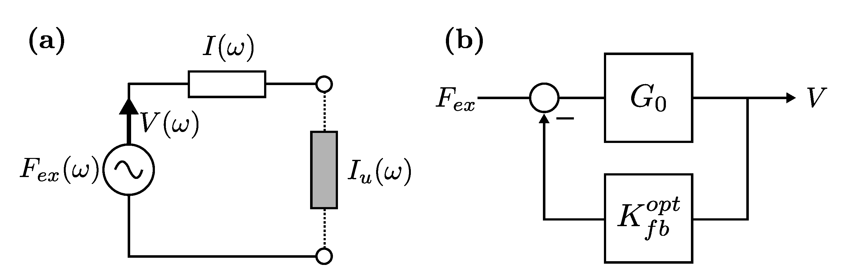
denotes the equivalent (intrinsic) impedance of the WEC. Naturally, Equation (8) resembles well-known representations in the field of electrical/electronic engineering and circuits theory: the WEC dynamics (7) can be equivalently represented by the analogue circuit that is depicted in Figure 1a.

In other words, the control input $F_u\left(\omega \right)$ can be considered as a load, which has to be designed, so that maximum power transfer is achieved from the source, i.e., the wave excitation input $F_{ex}\left(\omega \right)$. From this particular point of view, this problem can be directly addressed using the so-called impedance-matching (or maximum power transfer) theorem [7], which is a well-established result within the electrical/electronic engineering community. This theorem states that the load impedance, $I_u$, should be designed, for alternating (a.c.) circuits, such that it exactly coincides with the complex-conjugate of the source impedance, I. In other words, the control input that maximises power transfer, for the WEC case, is given by

$$F_u\left(\omega \right)=I_u\left(\omega \right)V\left(\omega \right)=I^{🟉}\left(\omega \right)V\left(\omega \right)=K_{fb}^{opt}\left(\omega \right)V\left(\omega \right),$$

(10)

where the notation $K_{fb}^{opt}$ is used to denote that the ‘controller’ in (10) is of a feedback-type. The result that is posed in (10) is indeed appealing, mainly due to its intrinsic simplicity, and its direct link to fundamental and well-established theory in the field of analogue circuits. Nevertheless, there are several issues that are associated with the control specifications given in (10), which prohibits the smooth application of what could potentially be an extremely appealing principle. These are listed and discussed in the following paragraphs.

To begin this discussion, note that the Laplace-transform analogue of Equation (7), when considering zero initial conditions, directly yields,

$$V\left(s\right)=G_0\left(s\right)\left[F_{ex}\left(s\right)-F_u\left(s\right)\right],$$

(11)

where the mapping $G_0:\mathbb{C}\to \mathbb{C}$, defining the input-output dynamics $f_{ex}-f_u\mapsto v$, is given by

$$G_0\left(s\right)={\displaystyle \frac{H_r^D\left(s\right)s}{(M+m_{\infty })H_r^D\left(s\right)s^2+H_r^N\left(s\right)s+H_r^D\left(s\right)s_h}},$$

(12)

where the Laplace transform of the radiation impulse response, $H_r$, has been written, without any loss of generality, as $H_r\left(s\right)=H_r^N\left(s\right)/H_r^D\left(s\right)$. Given the causality property of the radiation force system ${\mathsf{\Sigma }}_r$ (see, for instance, [16]), and the fact that ${\mathsf{\Sigma }}_r$ is always strictly proper [8], the following relation

$$\mathrm{deg}\left\{H_r^N\left(s\right)\right\}<\mathrm{deg}\left\{H_r^D\left(s\right)\right\},$$

(13)

holds. Direct observation of Equations (8) and (11) yields that, in the frequency-domain, the relation $I\left(\omega \right)=1/G_0\left(\omega \right)$, holds. In other words, the dynamical system that is associated with the frequency-response $I\left(\omega \right)$ is inherently non-causal, as a direct consequence of the fact that the transfer function $G_0\left(s\right)$ is strictly proper (see Equation (13)). This poses a major issue with respect to the applicability of result (10): the dynamical system that is associated with the control law (10) cannot be practically implemented, due to its intrinsic non-causality. In addition to this non-causality issue, the following additional implications that are associated with the matching-principle can be identified:

• The optimal control law (10) implies a different matching-condition for each input-frequency $\omega$.
• Neither device nor actuator limitations are observed by the matching condition (10). As a matter of fact, this control strategy often requires unrealistic displacement, velocity, and control input values to successfully achieve maximum power absorption. This is a direct product of the linearising assumptions under which Equation (6) is derived.
• The stability, sensitivity, and robustness properties of the control loop associated with the impedance-matching principle of (10), depicted in Figure 1b, have been recently questioned in [17]. In particular, [17] shows that radiation damping modelling errors can be particularly detrimental in the impedance-matching condition, given that a very specific zero-pole cancellation takes place when $f_u$ is selected, as in (10).

Note that the force-to-motion (force-to-velocity in this case) frequency-response mapping, under impedance-matching condition (10), can be readily computed as

$$V\left(\omega \right)={\displaystyle \frac{G_0\left(\omega \right)}{1+G_0\left(\omega \right)K_{fb}^{opt}\left(\omega \right)}}{F}_{ex}\left(\omega \right)={\displaystyle \frac{1}{2B_r\left(\omega \right)}}{F}_{ex}\left(\omega \right),$$

(14)

where $B_r$ is the radiation damping, as defined in Section 2. In particular, there exists an optimal real-valued scaling function $T^{opt}:\mathbb{R}\to {\mathbb{R}}^{+}$, which is given by

$$T^{opt}\left(\omega \right)={\displaystyle \frac{1}{2B_r\left(\omega \right)}}.$$

(15)

Note that the image of $T^{opt}$ is effectively contained in ${\mathbb{R}}^{+}$, as a consequence of the passivity property of the radiation force, i.e., $B_r\left(\omega \right)>0$, $\forall \omega \in \mathbb{R}/0$.

Although impedance-matching, as in (10), has some difficulties in practical application (for the reasons discussed above), it effectively describes the underlying dynamics behind maximum energy absorption, in an intuitive way. As a matter of fact, this principle underpins the family of simple controllers analysed in this study (see Table 2), which effectively attempt to provide implementable approximations of the control law derived in (10). The methodologies, which were employed by each of these five (5) controllers to approximate the impedance-matching condition (10), are discussed in detail in Section 4.

4. Simple WEC Controllers (in Chronological Order)

This section outlines the fundamentals behind each of the simple energy-maximising control strategies listed in Table 2, which are inherently based on the impedance-matching principle (as described in Section 3), proposed during the period between 2010–2020. In particular, the five (5) control strategies originally presented in [9,10,11,12,13], are recalled (in chronological order) in Section 4.1, Section 4.2, Section 4.3, Section 4.4 and Section 4.5, respectively. From now on, the shorthand notation introduced in Table 2 is used to refer to each specific strategy.

Note that this section does not simply recall results, but it also provides a critical analysis of each controller with respect to their potential success in a practical implementation, from a system dynamics perspective. In particular, the presented discussion aims to highlight the underlying simplicity of each presented controller, in terms of its applicability in the widest possible range of hardware platforms, including, for instance, low-cost microcontrollers. In the light of this, properties, such as nature of the control structure (i.e., linear, nonlinear, time-varying, etc.), as well as order, stability, and constraint handling capabilities (if any), are explicitly discussed, for each of the controllers that are listed in Table 2.

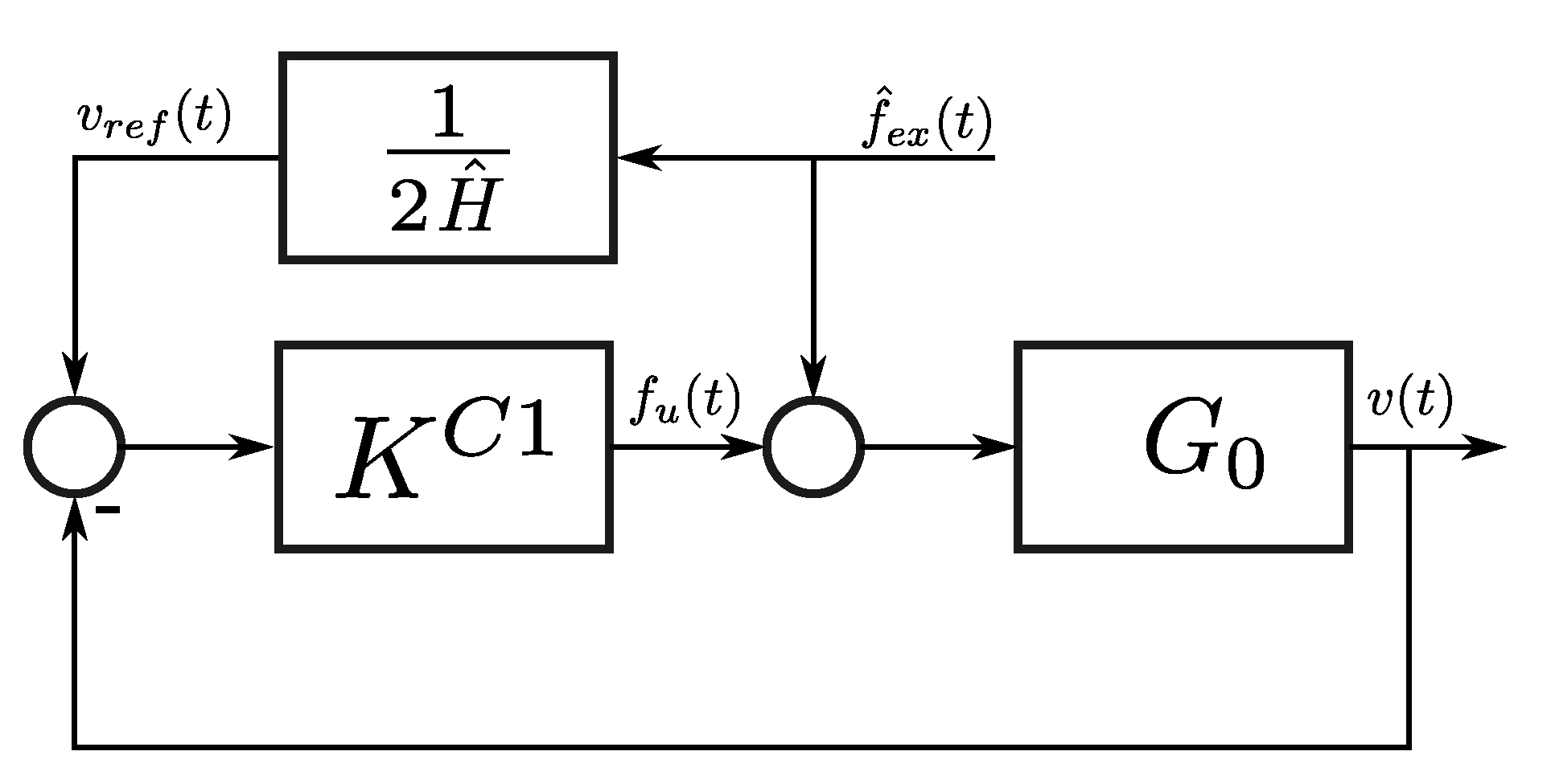
4.1. Suboptimal Causal Reactive Control (2011, C1)

This energy-maximising control strategy is essentially based on a velocity-profile tracking-loop (typical of approximate velocity tracking (AVT) WEC controllers [18]), schematically depicted in Figure 2, where ${\widehat{f}}_{ex}\left(t\right)$ indicates the estimation of the wave excitation force $f_{ex}\left(t\right)$. Using the fundamental impedance-matching principle and the optimal mapping $T^{opt}\left(\omega \right)$, as described in Equation (15), the control methodology presented in [9], although being suboptimal, represents a suitable methodology for real-time application, considering that only linear time-invariant (LTI) systems are involved in the control design procedure (further discussed in the following paragraphs). It should be noted that, even though this control methodology requires the estimation of the wave excitation force (to effectively compute the velocity profile $v_{ref}$), such an estimate can be obtained by means of standard unknown-input observers. This includes, for instance, Kalman-based estimators, in combination with a harmonic description of the wave excitation input [19].

Essentially, this control technique approximates the optimal mapping $T^{opt}\left(\omega \right)$ as follows:

$$T^{opt}\left(\omega \right)=\frac{1}{2B_r\left(\omega \right)}\approx \frac{1}{2\widehat{H}},$$

(16)

where $\widehat{H}\in {\mathbb{R}}^{+}$. In particular, the study that is presented in [9] computes the constant gain $\widehat{H}$ using a second order approximation of the force-to-velocity WEC model:

$$G_0\left(\omega \right)\approx {\tilde{G}}_0\left(\omega \right),$$

(17)

where ${\tilde{G}}_0:\mathbb{R}\to \mathbb{C}$ represents the frequency-response mapping of a second-order system, obtained by means of a model reduction routine that is based on Hankel singular values (see, for instance, [20]). Thus, if $G_0\left(\omega \right)\approx {\tilde{G}}_0\left(\omega \right)$, then the authors of the C1 controller rely on the following relation

$$B_r\left(\omega \right)\approx {\tilde{B}}_r=\widehat{H},$$

(18)

with ${\tilde{B}}_r\in {\mathbb{R}}^{+}/0$, being the approximation in Equation (18) valid (i.e., accurate) for a certain range of $\omega$.

Note that, in order to obtain a system ${\tilde{G}}_0\left(\omega \right)$ that satisfies Equation (18), while preserving the band-pass nature of the force-to-velocity mapping of a WEC system, a zero at the origin can be forced in the determination of ${\tilde{G}}_0\left(\omega \right)$. Nevertheless, only the order (number of eigenvalues) and stability of the approximating system can be handled using model reduction routines that are based on Hankel singular values. Note that, when the zero at the origin is guaranteed, and ${\tilde{G}}_0\left(s\right)$ consequently represents a band-pass structure, then:

$${\tilde{B}}_r=\mathbb{R}\mathrm{𝕖}\left\{\frac{1}{{\tilde{G}}_0\left(\omega \right)}\right\},$$

(19)

where ${\tilde{G}}_0\left(\omega \right)$ is, as a consequence of Equations (18) and (19), a passive system. However, in practical terms, the value of $\widehat{H}$ can be determined, depending on, for example, the spectral content of the sea-states characterising the operating conditions of the specific device being controlled. In other words, one can select $\widehat{H}$ merely as the radiation damping of the device, i.e., $B_r\left(\omega \right)$, evaluated at the frequency associated with the most energetic waves, in the total wave power spectrum.

It should be noted that, depending on the operating conditions (i.e., sea-states under analysis), the optimal $\widehat{H}$, which maximises the generated power for particular control specifications, can be potentially tuned while using a higher-order approximation of the WEC dynamics (rather than second-order, as per the original design behind the C1 controller). Furthermore, when considering that this control strategy can only interpolate the optimal condition at a finite number of frequencies3, then only monochromatic (regular) sea-states can be efficiently addressed, in terms of maximum theoretical power production, with this energy maximising control technique.

Concerning the stability of the C1 controller, note that the system $1/2\widehat{H}$ is an open-loop static mapping, and the definition of $\widehat{H}$ does not affect the stability of the complete control loop; therefore, $1/2\widehat{H}$ can be specifically tuned for different cases, considering a number of different design criteria, driven by the operating conditions.

On the other hand, under certain assumptions, which, when considering the passivity of $G_0\left(s\right)$, are guaranteed for WEC systems, the tracking feedback controller $K^{C1}$ (see Figure 2) can be synthesised, as suggested in [9], while using the Youla-Ku$\breve{\mathrm{c}}$era parametrisation for stable systems [21], i.e.,

$$K^{C1}\left(s\right)=\frac{Q\left(s\right)}{1-Q\left(s\right)G_0^{-1}\left(s\right)},$$

(20)

where $Q\left(s\right)=F\left(s\right)G_0^{-1}\left(s\right)$ and, for example,

$$F\left(s\right)=\frac{\frac{{\omega }_c}{q_f}s}{s^2+\frac{{\omega }_c}{q_f}s+{\omega }_c^2},$$

(21)

which represents a classical band-pass filter, such that $F\left({\omega }_c\right)=1$, and where $q_f\in {\mathbb{R}}^{+}/0$ indicates the band-width of the filter. However, note that the design of the internal tracking controller $K^{C1}$ can be performed using a wide variety of control techniques, including, for instance, ${\mathcal{H}}_{\infty }$-techniques, to cover system uncertainties, or sliding-modes methodologies, to tackle potential nonlinearities arising in the WEC dynamical system. From a stability perspective, which, as discussed in Section 3, represents a well-known issue in impedance-matching based controllers, this control strategy can be safely designed without compromising closed-loop stability.

Finally, note that this control strategy itself is purely based on LTI systems: both the computation of the reference velocity profile, $v_{ref}$, and the tracking controller, $K^{C1}$, involve LTI systems. Regarding the order of the C1 controller when the above Youla-Ku$\breve{\mathrm{c}}$era parametrisation technique is considered, i.e., Equations (20) and (21), the order of the controller $K^{C1}\left(s\right)$ is given by $n+1$, where n denotes the order of the WEC model $G_0\left(s\right)$.

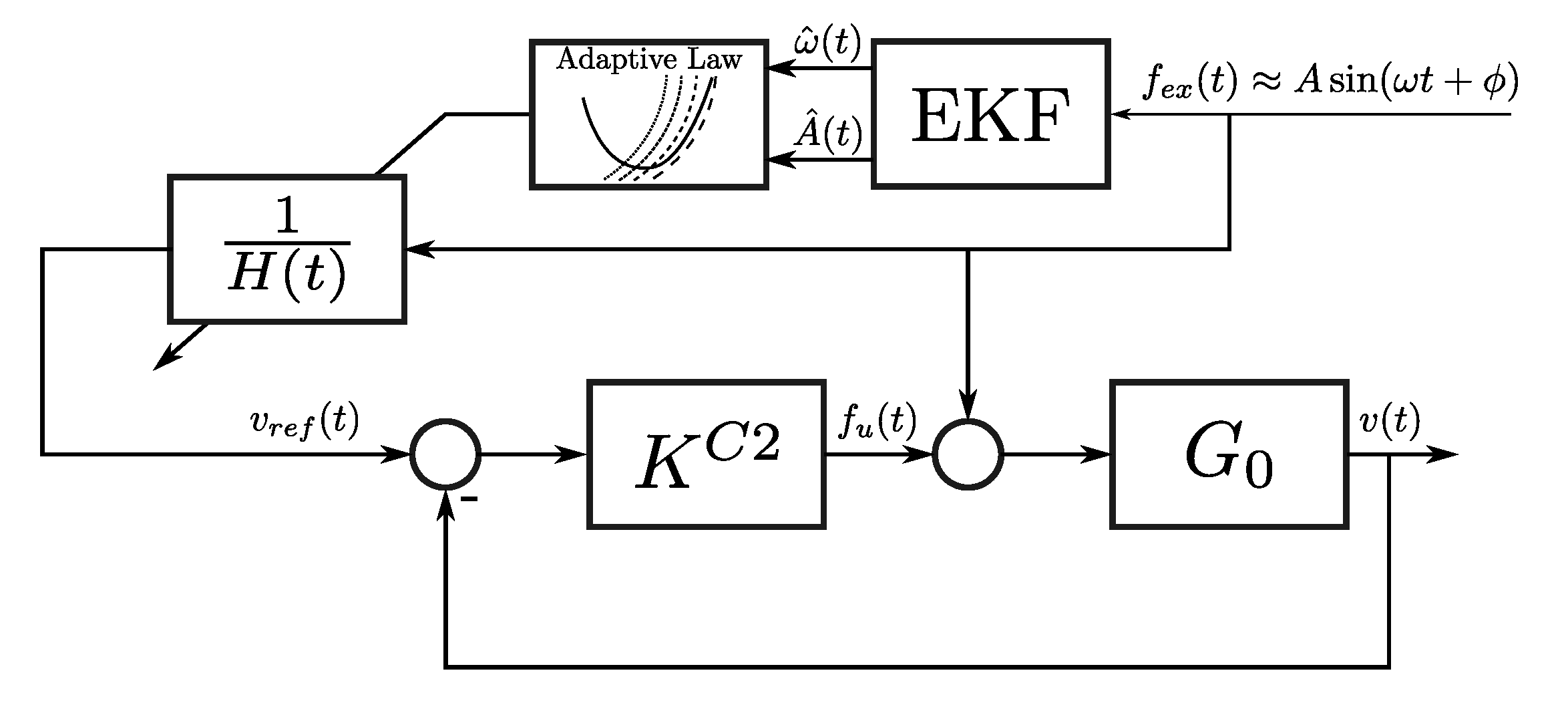
4.2. Simple and Effective Real-Time Controller (2013, C2)

The C2 controller, as schematically depicted in Figure 3, has one particular appealing feature: It not only provides a simple a approximation of the impedance-matching principle, but also incorporates a constraint handling mechanism. This controller, together with the C5 (see Section 4.5), are the only two simple controllers presented in the literature which are capable of handling physical constraints as part of their design.

The C2 controller arises as an extension of the controller presented in [9], as detailed here in Section 4.1. In particular, the wave excitation force, as considered for this control strategy, is approximated using a monochromatic sinusoidal process, i.e.,

$$f_{ex}\left(t\right)\approx A\left(t\right)sin(\omega \left(t\right)t+\varphi \left(t\right)),$$

(22)

with parameters $\{A,\omega ,\varphi \}\subset \mathbb{R}$, which can vary with time. Similarly to the C1 controller, the C2 is essentially based on a velocity-profile tracking-loop (AVT controller). Unlike its predecessor, the C2 strategy features an adaptive process, where the velocity reference profile is updated in real time by means of an Extended Kalman filter (EKF), which provides an instantaneous estimate of the set of parameters $\{A,\omega ,\varphi \}$, fully characterising the excitation force as in (22). Such an estimation is motivated by two clear objectives, as detailed in the following. Firstly, knowledge of these estimates is used to improve the block $\frac{1}{2\widehat{H}}$ that is proposed in the C1 controller (as shown in Figure 2), by means of a continuous-time adaptation procedure, aiming to approach the optimal condition $T^{opt}\left(\omega \right)$, stated by the impedance-matching principle. Secondly, the information provided by the estimation is used to normalise the wave excitation force estimate and compute a suitable velocity profile, according to pre-defined constraint specifications. To be precise, the information provided by the EKF is explicitly employed in the computation of the following time-varying scaling function:

$$\frac{1}{H\left(t\right)}=\left\{\begin{array}{ccc}\frac{1}{2B_r\left(\widehat{\omega }\left(t\right)\right)},& \mathrm{if}& \frac{\widehat{\omega }\left(t\right)X_{lim}}{\widehat{A}\left(t\right)}>\frac{1}{2B_r\left(\widehat{\omega }\left(t\right)\right)},\\ \frac{\widehat{\omega }\left(t\right)X_{lim}}{\widehat{A}\left(t\right)},& \mathrm{if}& \mathrm{otherwise},\end{array}\right.$$

(23)

where $X_{lim}$ represents the maximum displacement limit. Such a mapping $H\left(t\right)$ is schematically shown in Figure 3, where $\widehat{A}\left(t\right)$, $\widehat{\omega }\left(t\right)$ represent the instantaneous estimates of amplitude A and frequency $\omega$, both in Equation (22), respectively. Finally, the feedback tracking controller, denoted as $K^{C2}$ in Figure 3, can be computed while using the Youla-Ku$\breve{\mathrm{c}}$era parametrisation, as per the case of the C1 controller, described in Section 4.1. To be precise, the controller $K^{C2}$ can be designed following the expressions provided in Equations (20) and (21). It is important to highlight that, although the estimation process in the C2 controller is performed in terms of an EKF, a wide variety of estimation techniques could be potentially employed to provide instantaneous estimates of A and $\omega$ (see, for instance, [19]).

There are some aspects, both positive and negative, related to the C2 controller, and its applicability in realistic environments, which are worth mentioning. On the positive side, the C2 controller can effectively handle displacement limitations in terms of the design parameter $X_{lim}$. This is clearly fundamental in any practical application, where compliance with physical restrictions must be guaranteed by the energy-maximising control strategy, hence maximising energy absorption while minimising the risk of component damage. Nonetheless, on the negative side, and taking into account the challenge involved in the tuning of the corresponding estimator, and its sensitivity to design parameters [19], the inclusion of the EKF can potentially impact (negatively) on the resulting performance, as detailed in the following. In particular, when considering that the wave excitation force can be expressed as in Equation (22), methodologies that instantaneously estimate the amplitude A and frequency $\omega$, virtually always assume that A is approximately constant. In addition, the computation of an estimate of the frequency $\omega$, in Equation (22), inherently requires a non-linear estimation process [19]. The necessity of assuming a low variation rate for the amplitude modulation $A\left(t\right)$ (see [19]), and the fact that the design and calibration of the nonlinear estimation process that is required to compute the instantaneous input frequency is substantially challenging, can potentially degrade the quality of the approximating $f_{ex}$ defined in (22). This naturally has a direct impact on the quality of the energy-maximising solution provided by the C2 controller (which explicitly uses this estimate in order to compute the corresponding control force), both in terms of performance, and satisfaction of physical limitations (i.e., constraints).

From a stability analysis point of view, this controller presents an advantage, directly related to the simple LTI velocity tracking controller $K^{C2}$: In other words, one can always guarantee stability in the C2 controller as long as the tracking loop is stable, and the EKF strategy converges towards a bounded wave excitation estimate. However, even though the reference tracking controller is based on a LTI system, this control methodology cannot be considered LTI altogether, due to the presence of the time-varying prefilter $1/H\left(t\right)$, which is involved in the computation of the velocity profile $v_{ref}$. Regarding the feedback controller order, when the Youla-Ku$\breve{\mathrm{c}}$era parametrisation is considered (i.e., as in Equations (20) and (21)), the order of $K^{C2}\left(s\right)$ is given by $n+1$, where n denotes the order of the WEC model $G_0\left(s\right)$. Finally, note that convergence of the EKF estimation, towards the real wave excitation force time-trace, cannot be generally guaranteed, mainly because such a force cannot be always expressed as in Equation (22). In other words, this controller inherently assumes that the device is subject to waves that arise from a narrowbanded sea-state, which is not always the case in practice.

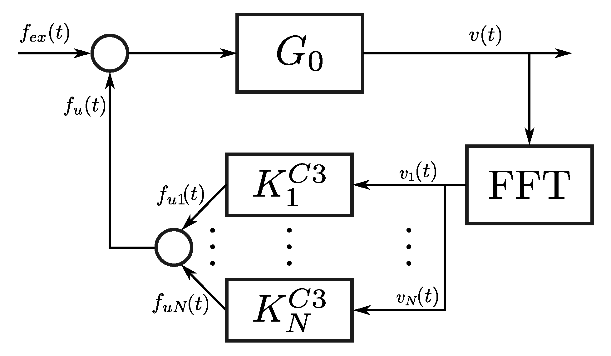
4.3. Multi Resonant Feedback Control (2016, C3)

The controller that is presented in [11], i.e., the C3 controller, is strictly based on a feedback structure. It is important to note that, in contrast to the previously presented two controllers (Section 4.1 and Section 4.2), the feedback structure does not require wave excitation force estimates, which positively impacts on its associated computational complexity. Aiming to address the energy-maximisation problem in a broadband sense, the design of the C3 controller is based on a specific approximation of the impedance-matching condition using a frequency-domain discretisation, i.e., considering a finite set of frequencies as,

$$\mathsf{\Omega }=\left\{{\omega }_1,\cdots ,{\omega }_N\right\}\subset {\mathbb{R}}^{+}.$$

(24)

To this end, and similarly to the case that is presented in Section 4.2, the wave excitation force is approximated as a finite sum of N purely sinusoidal processes, i.e.,

$$f_{ex}\left(t\right)\approx \sum _{i=1}^N{A}_i^{ex}sin({\omega }_{i}t+{\varphi }_i^{ex}).$$

(25)

Subsequently, given the linearity associated with the WEC model $G_0\left(s\right)$, the device velocity can be consequently described as:

$$v\left(t\right)\approx \sum _{i=1}^N{v}_i\left(t\right)=\sum _{i=1}^N{A}_{i}sin({\omega }_{i}t+{\varphi }_i).$$

(26)

Note that the C3 control strategy, as presented in [11], uses position as the default output of the WEC system $G_0\left(s\right)$. However, aiming to be consistent with all the (other) controllers that are considered in this study, and without any loss of generality, the velocity is used in this study as the output of the WEC system. Figure 4 schematically depicts the C3 control strategy.

As a consequence of the assumption regarding the wave excitation force and velocity stated in Equations (25) and (26), the authors of [11] separate the system $G_0\left(s\right)$ into N second-order subsystems, i.e., ${\left\{G_i\left(s\right)\right\}}_{i=1}^N$, such that

$$G_0\left({\omega }_i\right)=G_i\left({\omega }_i\right),$$

(27)

for all ${\omega }_i\in \mathsf{\Omega }$, with $i\in {\mathbb{N}}_N$. The objective sought with the separation, as shown in Equation (27), is to deal with simpler individual systems $G_i\left(s\right)$ where, given the second-order nature of each subsystem $G_i\left(s\right)$, the following result

$$\mathbb{R}\mathrm{𝕖}\left\{\frac{1}{{\tilde{G}}_0\left(\omega \right)}\right\}=B_r^i,$$

(28)

with $B_r^i\in {\mathbb{R}}^{+}$, for all $i\in {\mathbb{N}}_N$, holds. The relation that is posed in Equation (28) is a key factor in the definition of the optimal control condition exploited by the C3 controller: instead of solving the complete energy maximising control problem, i.e., considering the optimal frequency-domain impedance-matching condition for all $\omega \in \mathbb{R}$, the C3 control strategy aims to solve the impedance-matching problem for each subsystem $G_i\left(s\right)$, which is intrinsically related to each $B_r^i$, defined in Equation (28). In particular, the energy-maximising control problem is tackled while using a set ${\mathbf{K}}^{C3}$ of N proportional-integral (PI) controllers, i.e., ${\mathbf{K}}^{C3}={\left\{K_i^{C3}\left(s\right)\right\}}_{i=1}^N$, with each $K_i^{C3}$ defined as

$$K_i^{C3}\left(s\right)=\left(P_i^{C3}+\frac{I_i^{C3}}{s}\right),$$

(29)

where the set of parameters ${\{P_i^{C3},I_i^{C3}\}}_{i=1}^N\subset \mathbb{R}$ is designed to approach the impedance-matching optimal condition for each subsystem $G_i\left(s\right)$.

Note that the control problem that is posed in [11] is stated as an optimisation problem, where the values $A_i$ and ${\varphi }_i$, as expressed in Equation (26), are estimated in real-time. In other words, the determination of the instantaneous estimate of each $A_i$ and ${\varphi }_i$, in Equation (25), plays a key role in this control strategy, and is addressed by the C3 in terms of an optimisation problem. In particular, the estimation required in [11] is tackled by means of a real-time implementation based on the fast Fourier transform (FFT), as shown in Figure 4. Note that different (time) window lengths are utilised in the case studies that are presented in [11], aiming to analyse their effect in the final energy-maximising performance.

From a general perspective, mainly concerning the applicability and the stability of this control strategy, some aspects are worth mentioning. Firstly, the use of a real-time FFT and the time window required for its implementation generates a time-delay between measurement and control actuation. It is important to highlight that time precision plays a decisive role in real-time implementation, and can intrinsically affect both the stability properties of the control loop, and its performance in terms of energy capture. By the way of example, and in order to highlight the importance of having good timing in realistic control implementations, the use of a real-time operating system (RTOS), such as, for example real-time LabView, Matlab xPC Target, RTOSs for the microcontroller architecture, or even FPGA-based systems, is a common practice for realistic control implementation. This effectively reduces the time-delay between measurement and control actuation (i.e., latency or jitter). Note that the FFT procedure can be potentially replaced by suitable recursive least square (RLS) routines, such as those that are described in [22]4. This allows for a potentially more computationally efficient implementation than its FFT counterpart, which would be appealing for real-time applications. Secondly, the methodology that is employed in [11] to define $G_i\left(s\right)$ is not clearly stated. Note that there exists an infinite number of possible second-order systems $G_i\left(s\right)$ fulfilling Equation (27), which can lead to different control scenarios. In addition, even though a stability analysis is performed in [11] while using the classical Routh–Hurwitz criterion (see, for instance, [23]) for each controller-plant pair $(K_i^{C3},G_i)$, it is not clear how the stability of the complete interconnection, i.e., $({\mathbf{K}}^{C3}$, $G_0)$, can be guaranteed. Furthermore, the authors of [11] do not take into account the estimation of each $A_i$ and ${\varphi }_i$ in the closed-loop stability analysis, which further increases the degree of uncertainty behind the practicality of this solution. Note that such an estimation process depends upon a time-dependent optimisation routine, which automatically renders the control loop as time-varying, commonly requiring converse Lyapunov theory (see, for instance, [24]) to guarantee uniform stability, which intrinsically complicates the nature of the problem.

Finally, note that this controller cannot be considered a LTI system, due to the optimisation process that is involved in the feedback path. In addition, regarding the order of the set of controllers ${\mathbf{K}}^{C3}$, when considering the PI structure presented in Equation (29), the total order always matches the number of elements considered in the frequency set $\mathsf{\Omega }$, i.e., there is one PI (first-order) controller for each element of the set $\mathsf{\Omega }$.

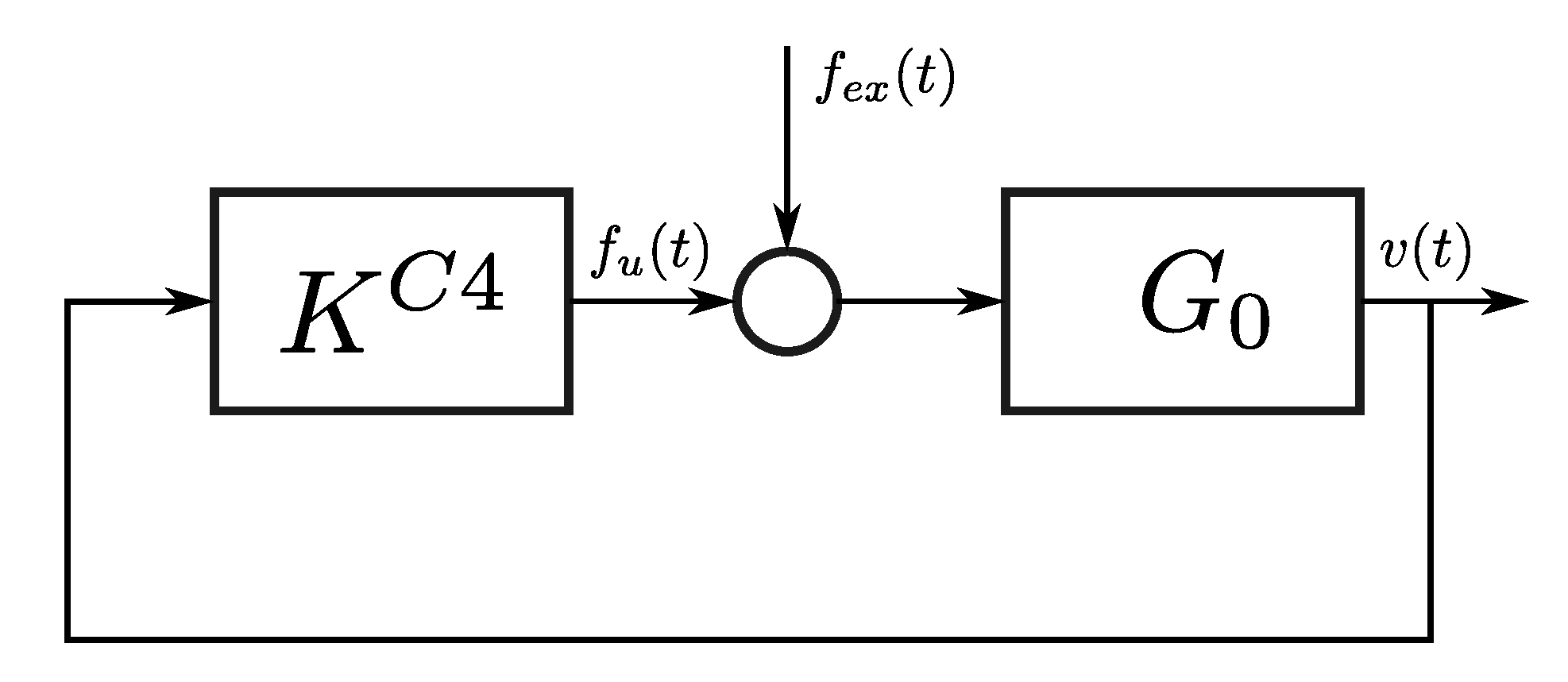
4.4. Feedback Resonating Control (2019, C4)

As in the case detailed in Section 4.3, the energy maximising control strategy presented in [12], denoted here as C4, is essentially based on a classical feedback control structure, as depicted in Figure 5. Thus, as for the C3 controller, knowledge of the wave excitation force is not required to implement the C4 control strategy, which significantly reduces the controller complexity and simplifies its implementation, as well as contributing to improving the resulting performance, as long as some guarantee of closed-loop stability can be provided.

In the energy-maximising control strategy proposed in [12], the controller is synthesised while using system identification algorithms, aiming to approximate the frequency-domain feedback optimal control condition, i.e., Equation (10). The control strategy is schematically depicted in Figure 5. In particular, the proposed controller has a fixed rational polynomial structure, as follows

$$K^{C4}\left(s\right)=\frac{b_2{s}^2+b_{1}s+b_0}{s^2+a_{1}s+a_0},$$

(30)

which structurally considers two poles and two zeros, with $\{b_{0,}{b}_1,b_2,a_0,a_1\}\subset \mathbb{R}$. Subsequently, in order to approximate the impedance-matching optimal condition over a certain frequency range, the system in Equation (30) is designed to satisfy the following relation:

$$K^{C4}\left(\omega \right)\approx K_{fb}^{opt}\left(\omega \right).$$

(31)

with $K_{fb}^{opt}\left(\omega \right)$ defined in Equation (10). Given that input-output stability can be generally set as a requirement in the majority of standard identification approaches available in the literature [25], the stability of the controller can be straightforwardly satisfied, which is recommended for any realistic control system implementation. However, this does not necessarily guarantee closed-loop stability for the system that is depicted in Figure 5; additional requirements need to be imposed on the structure in (30) in order to secure stable closed-loop behaviour, such as, for instance, passivity.

In addition, the simplicity of the controller structure, given its second-order nature, is worth highlighting. Furthermore, recalling that stability represents a key issue for controllers that are based on the impedance-matching principle, the C4 control methodology can be relatively easily designed in order to guarantee both controller and, more important, closed-loop, stability, although the latter is not theoretically addressed in [12]. Nevertheless, the lack of a constraint handling mechanism can render the C4 controller unsuitable for realistic implementations.

From a dynamical systems perspective, this controller is based on a single LTI system. In addition, considering the fixed structure that is presented in Equation (30), the controller order is always set to 2.

4.5. LiTe-Con (2020, C5)

Similarly to the case that is presented in Section 4.4, the so-called LiTe-Con [13] (referred to here as C5), is synthesised using system identification algorithms, aiming to approximate the frequency-domain energy-maximising optimal condition. In particular, based on the impedance-matching feedback law (10), in order to provide an alternative energy maximising control solution that is capable of dealing with the stability issues detailed in Section 1, the authors of [13] recast the controller solution into an equivalent feedforward structure, i.e.,

$$K_{ff}^{opt}\left(\omega \right)=\frac{\mathbb{R}\mathrm{𝕖}\left\{G_0\left(\omega \right)\right\}+j\mathbb{Im}\left\{G_0\left(\omega \right)\right\}}{2\mathbb{R}\mathrm{𝕖}\left\{G_0\left(\omega \right)\right\}},$$

(32)

where the mapping $f_{ex}\mapsto v$, corresponding with the feedforward structure (32), is equivalent to that presented in Equation (15). Note that, in contrast to C4, which does not require estimation of the wave excitation force, the feedforward control structure requires the estimation of the excitation force of the wave. Thus, the requirement of having an estimate of $f_{ex}\left(t\right)$, can negatively impact on the resulting performance [26]. The aspect that is related to the requirement of having an estimate of the wave excitation force can be considered as the essence of the distinction between C4 and C5. The non-parametric frequency-response mapping $K_{ff}^{opt}$ is then approximated by means of black-box system identification techniques, as further discussed in the upcoming paragraphs.

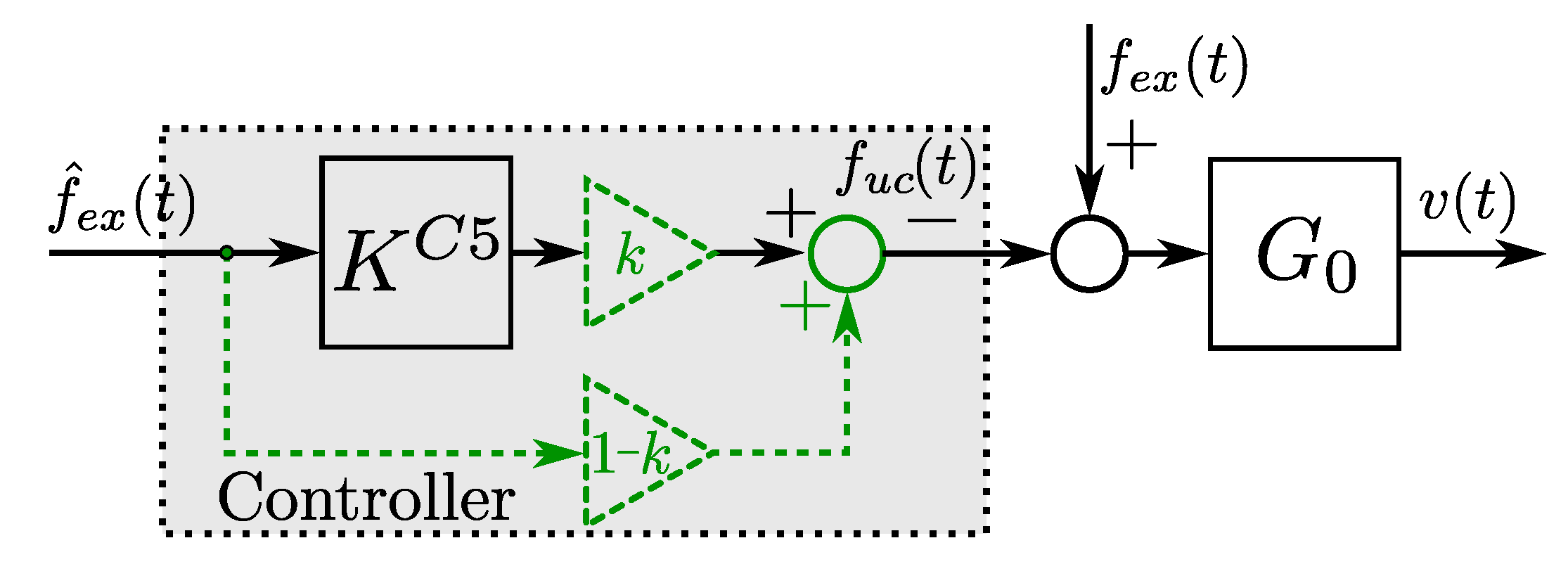
Given the inherent feedforward structure of the C5 controller, estimation of the wave excitation force is required. The control structure C5, as presented in [13], is schematically depicted in Figure 6, where ${\widehat{f}}_{ex}$ denotes the estimate of the wave excitation force $f_{ex}$, and $K^{C5}$ is the C5 controller. Note that a constraint handling mechanism is proposed in C5, extending its applicability range to realistic environments.

The controller methodology that is presented in [13] proposes the approximation of the optimal impedance-matching controller $K_{ff}^{opt}$, as defined in Equation (32), with a LTI-stable and implementable dynamical system $K^{C5}$, such that

$$K^{C5}\left(s\right){|}_{s=jw}\approx K_{ff}^{opt}\left(\omega \right),$$

(33)

where $K^{C5}\left(s\right)$ is obtained using frequency-domain system identification algorithms, such as subspace [25] or moment-matching-based [27] system identification techniques. Subsequently, the resulting control force (in the frequency domain) is expressed as:

$$F_u\left(\omega \right)=K^{C5}\left(\omega \right){\widehat{F}}_{ex}\left(\omega \right).$$

(34)

In order to implement the synthesised C5 controller in a realistic environment, a constraint handling mechanism is essential to prevent inflicting damage on the mechanical system. In particular, [13] proposes a constraint handling mechanism, using a constant value $k\in \left[0,1\right]$, so that the control force $F_u$ in Equation (34) is redefined as:

$$F_{uc}\left(\omega \right)=\underset{\mathrm{Controller}}{\underbrace{\left[k{K}^{C5}\left(\omega \right)+(1-k)\right]}}{\widehat{F}}_{ex}\left(\omega \right),$$

(35)

where it is straightforward to check that $F_{uc}\left(\omega \right)=F_u\left(\omega \right)$ when $k=1$. Assuming perfect matching in Equation (33), the optimal mapping in Equation (15) can be defined as:

$$T^{C4}\left(\omega \right)=k\left(\frac{{\mathbb{R}\mathrm{𝕖}\left\{G_0\left(\omega \right)\right\}}^2+\mathbb{Im}{\left\{G_o\left(\omega \right)\right\}}^2}{2\mathbb{R}\mathrm{𝕖}\left\{G_0\left(\omega \right)\right\}}\right).$$

(36)

Note that, if $k=1$ in Equation (36), then the optimal condition in Equation (15) is obtained, i.e., $T^{C4}\left(\omega \right)=T^{opt}\left(\omega \right)$. On the other hand, if $k=0$, then $T^{C4}\left(\omega \right)=0$. In other words, the inclusion of the term k allows for a simple implementation of position and velocity constraints, effectively constraining the position and velocity between zero and their theoretical maxima. The constraint handling mechanism of the C5 is indicated in Figure 6 using a dotted-grey box, while dashed-green lines are used to represent the internal block interconnections.

Some comments that are related to this control strategy and its applicability, particularly focusing on stability features, can be mentioned. On the positive side, the feedforward nature of the C5 controller requires a simple and relatively effortless implementation in real-world applications, while also effectively taking into account device limitations in terms of a simple constraint mechanism. Nonetheless, the C5 controller requires an estimate of the wave excitation force, which can potentially have a negative impact on the energy-maximising performance of the controller [28] and computational complexity. However, in contrast to, for instance, the C2 controller (which uses requires an EKF structure), the estimation that is required by the C5 can be addressed while using relatively standard wave excitation force estimation techniques. In particular, a LTI Kalman filter5, featuring a harmonic description for ocean waves, is considered in [28]. As demonstrated in [19], this observer provides good overall estimation quality, while inherently handling measurement noise (in an optimal sense). From a stability perspective, the complete control structure stability (WEC system, excitation force estimator, and controller) is guaranteed as long as each individual component (WEC model, estimator, and controller) is stable, i.e., under the separability principle [23].

Finally, note that this control strategy is purely based on LTI systems (even taking into account the required estimation process for the wave excitation force). Regarding the order of the controller, it directly depends upon the system identification process that is employed to compute $K^{C5}$. For instance, using a moment-based identification approach [27], where the user can select a number of interpolation frequencies (or points) to preserve steady-state response characteristics (see Section 5.1.5), the order of the controller $K^{C5}$ is twice the number of matching points.

5. Results

This section presents a case study, where the performance obtained with the set of five (5) controllers presented in Section 4, i.e., C1, C2, C3, C4, and C5, is assessed. Aiming to provide a set of benchmark cases in terms of maximum achievable absorbed energy, two reference measures are considered. Firstly, for the unconstrained case, the performance that is obtained with each controller is compared with the corresponding theoretical maximum, which is analytically computed while using Equation (15). Such a benchmark case is denoted here as CR1. Secondly, in the constrained case, where, unlike its unconstrained counterpart, there is not an explicit analytical formulation for the maximum achievable performance, an optimisation-based controller is considered. Even though the resulting performance that is obtained with optimisation-based formulations is not a theoretical maximum per-se (due to any potential errors arising from the intrinsic necessity of discretisation and use of numerical routines), it is considered here as a surrogate reference for maximum achievable performance in a constrained scenario. In particular, a moment-based controller [29], denoted in this study as CR2, is considered in this application case for the performance comparison in the constrained case, analogously to the performance assessment that is presented in [13]. It is important to note that, for the constrained case, only the C2 and C5 control methodologies can be considered for the performance assessment presented in this section: the controllers C1, C3, and C4 do not provide any constraint handling mechanism at all, which directly compromises their application in realistic scenarios. This is further discussed in the following paragraphs.

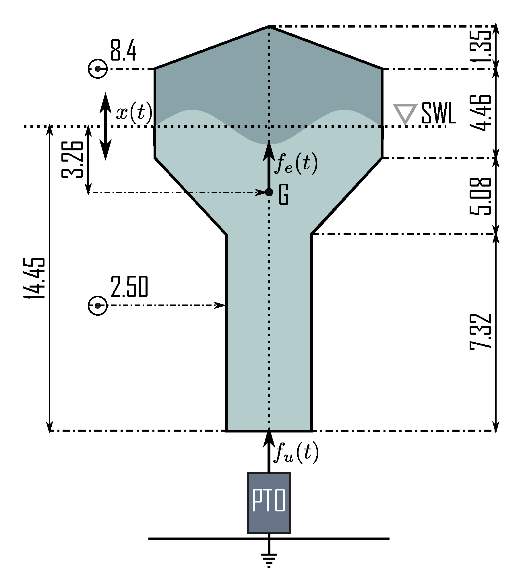
The control strategies are applied to a state-of-the-art full-scale CorPower-like device oscillating in heave (translational motion) [30]. This type of device is often considered throughout the WEC literature, being one of the most well-established WEC system within the wave energy field (see, for example, [31] or [32]), and it is illustrated in Figure 7 with its corresponding physical dimensions specified in meters. To perform the simulations and analysis shown in this section, the considered the WEC model, as in Figure 7, is described using an seventh-order LTI state-space representation, which is denoted in the frequency-domain as $G_0\left(\omega \right)$.

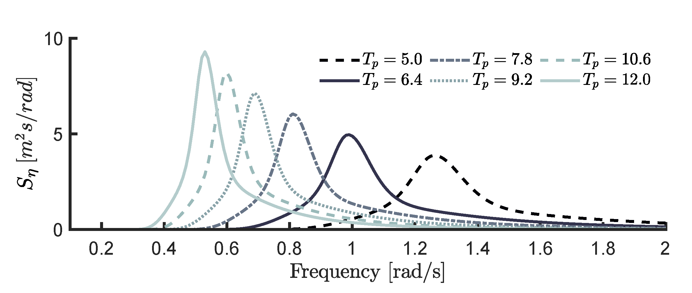
In this application case, the time-trace of the wave excitation force, $f_{ex}\left(t\right)$, considering irregular waves, is determined from the so-called free-surface elevation, $\eta \left(t\right)$, based on a JONSWAP spectrum $S_{\eta }\left(\omega \right)$ [33]. The corresponding sea-state parameters, which characterise the nature of the mapping $S_{\eta }$, are as follows: Peak period in the interval $T_p\in \left[5.0,12.0\right]$ s, significant wave height $H_s=2.0$ m, and a peak-enhancement factor $\gamma =3.3$. In Figure 8, $S_{\eta }\left(\omega \right)$ is depicted for $T_p=\left\{5,6.4,7.8,9.2,10.6,12\right\}$ s, where $T_p=5$ s and $T_p=12$ s indicate the extremes of the considered range for $T_p$.

The power spectral density of the excitation force is given by the relation $|F_{ex}\left(\omega \right)|=|G_{\eta }\left(\omega \right)\left|\right|S_{\eta }\left(\omega \right)|$, where $G_{\eta }\left(\omega \right)$, obtained using NEMOH [34], represents the frequency-response function associated with the mapping $\eta \mapsto f_{ex}$. The resulting performance is studied in both unconstrained, and constrained, scenarios, as detailed previously in this same section. In particular, in the constrained case, the maximum allowed displacement is set to $X_{max}=1.5$ m. In this study, $\eta \left(t\right)$ is generated using a white noise signal, filtered according6 to the spectrum $S_{\eta }\left(\omega \right)$ [35].

Throughout this section, performance is assessed in terms of the average absorbed power, which is evaluated as

$$P_{abs}=-\frac{1}{T}{\int }_0^T{f}_u\left(t\right)v\left(t\right)dt.$$

(37)

Note that, when considering the stochastic nature of the process involved, and to be statistically consistent, the results that are shown in this study are always representative average values, which are generated when considering 20 realisations of each specific sea-state.

Controllers C1, C2, and C5 require (potentially different) wave excitation force estimation procedures, as detailed throughout Section 4. For the case of C1 and C5, which rely upon an instantaneous estimate of the excitation force time-trace $f_{ex}\left(t\right)$, a linear Kalman filter is utilised, in combination with the internal model principle of control theory [36]. The design and synthesis procedure for such an observer, which is based upon a harmonic internal description of ocean waves, is well-established in the literature of WEC control, and it can be consulted elsewhere (see, for instance, [19]). Note that, in this study, the infinite-horizon Kalman gain is always utilised, i.e., the solution to the infinite-horizon algebraic Riccati equation, which directly implies that the associated estimator is LTI. The estimation requirements for controller C2 are different, and more ‘sophisticated’ methods than those associated with C1 and C5 are needed. In particular, this strategy relies upon having estimates of instantaneous amplitude $\widehat{A}\left(t\right)$ and frequency $\omega \left(t\right)$, which, as previously discussed, inherently require a nonlinear estimation procedure, given the nature of the internal model used to describe the wave excitation force (see Equation (22)). As detailed in Section 4.2, an EKF is, as proposed in [10], considered to perform this task7, which is designed and tuned following [10].

Although beyond the scope of this study, where ‘idealised’ conditions are assumed for simulation to guarantee a level playing field for the totality of the controllers studied, i.e., perfect knowledge of the WEC dynamics and noise-free measurements are considered, the reader is referred to, for instance, [17], for further detail on the impact of modelling mismatch in both feedback and feedforward structures, and [19,28], for potential performance deterioration caused by noisy measurements in wave excitation force estimators.

The remainder of this section is organised, as follows. Section 5.1 presents the design procedure of each controller recalled in Section 4. Section 5.2.1 and Section 5.2.2 show the performance results for each controller, in both unconstrained, and constrained scenarios, respectively, while Section 5.3 discusses the time-domain behaviour obtained with each controller.

5.1. Design Procedures

This section outlines the design procedure of each controller presented in Section 4. Throughout the following paragraphs, detailed comments and insight, with respect to design process, are also included, when appropriate.

5.1.1. C1

The design procedure for the C1 controller, as presented in Section 4.1, can be separated into two clear stages. Firstly, the constant function $1/2\widehat{H}$ has to be designed, so that a suitable velocity reference $v_{ref}$ is generated. The second stage involves the design and synthesis of a closed-loop controller, which is able to track such a velocity reference profile.

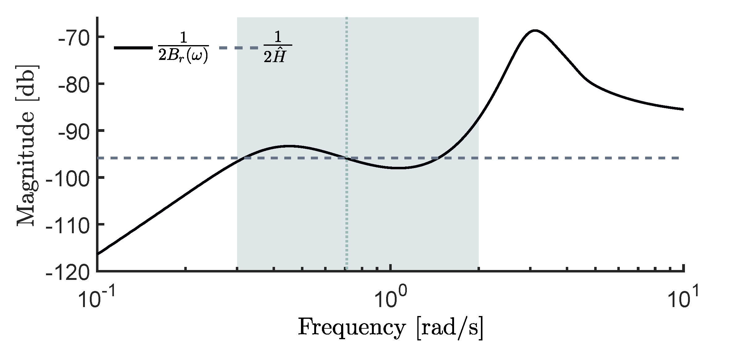
To approximate the optimal mapping $T^{opt}\left(\omega \right)$, in terms of $1/2\widehat{H}$, note that the waves that are considered in this study are generated using a stochastic description with peak period $T_p\in \left[5,12\right]$ s, i.e., waves with significant energy components in a frequency range of approximately $[0.3,2]$ rad/s (see Figure 8). Motivated by this, the value of $\widehat{H}$ is determined to be as representative as possible in such a frequency range, as depicted in Figure 9. In particular, the obtained $1/2\widehat{H}$ is shown using a dashed line, while the optimal mapping $T^{opt}\left(\omega \right)$ is depicted with solid line.

Note that, in Figure 9, the mean period $T_p=8.5$ s (which is obtained as the average between the extreme of the complete range) is depicted using a dotted line. Additionally, the corresponding frequency range, i.e., $\approx [0.3,2]$ rad/s, is depicted with a grey box. By the direct observation of Figure 9, one can appreciate that the best approximation of this optimal mapping $T^{opt}\left(\omega \right)$, provided by the constant gain $\widehat{H}$, happens precisely at $2\pi /8.5$ rad/s, i.e., the C1 controller interpolates $T^{opt}\left(\omega \right)$ at $T_p=8.5$ s.

As can be directly recalled from Section 4.1, the design procedure that is associated with the reference tracking loop is addressed while using a standard Youla-Ku$\breve{\mathrm{c}}$era parametrisation for stable systems, which can be directly considered for the WEC case due to its passive and non-minimum phase nature [8]. To be precise, the velocity tracking loop, as depicted in Figure 2, can be synthesised using the following structure:

$$K^{C1}\left(s\right)=\frac{Q\left(s\right)}{1-Q\left(s\right)G_0{\left(s\right)}^{-1}},$$

(38)

where $Q\left(s\right)=F\left(s\right)G_0{\left(s\right)}^{-1}$ and

$$F\left(s\right)=\frac{\frac{{\omega }_c}{q_f}s}{s^2+\frac{{\omega }_c}{q_f}s+{\omega }_c^2},$$

(39)

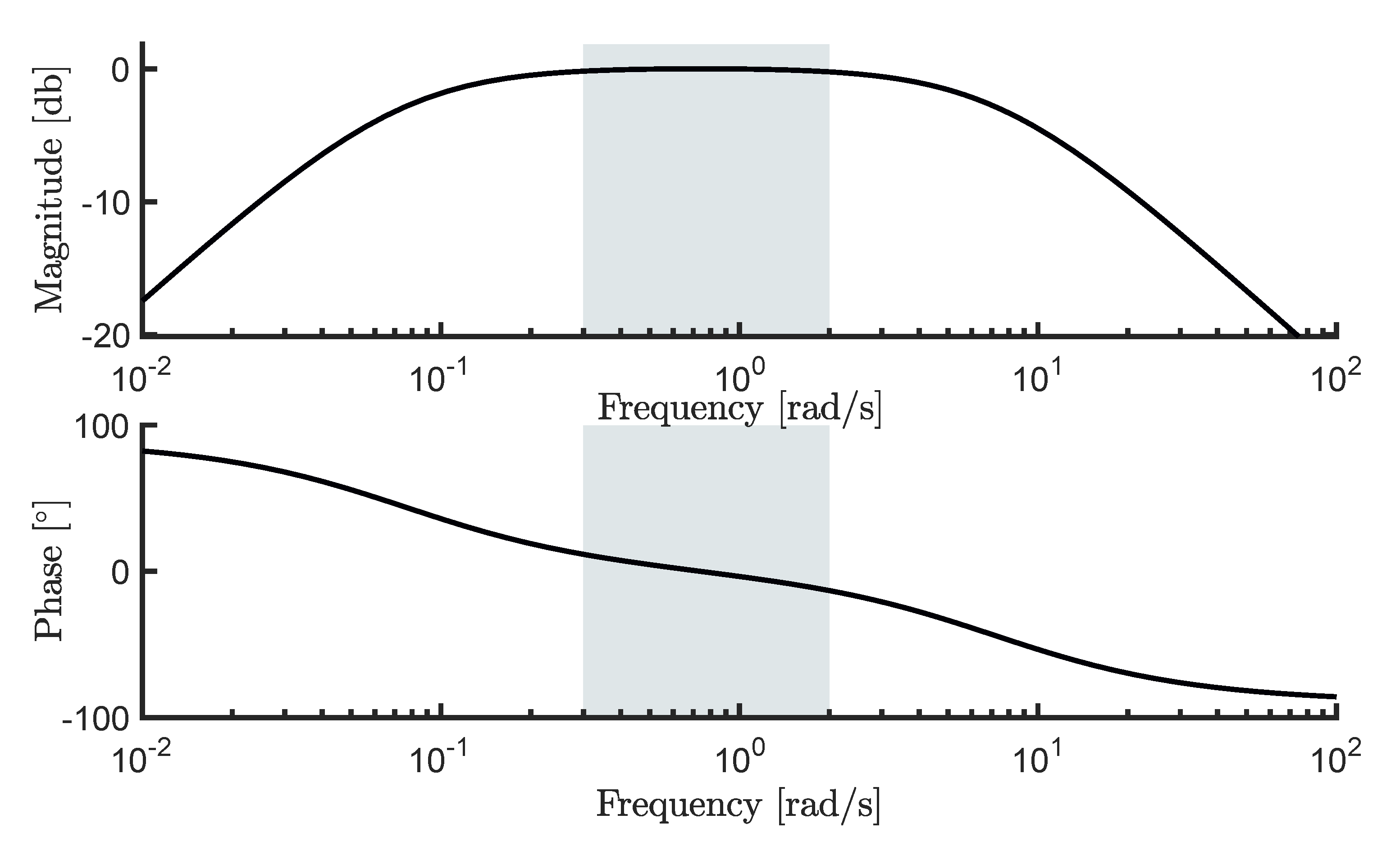
with ${\omega }_c=2\pi /8.5$ and $q_f=0.1$. Thus, a LTI feedback controller $K^{C1}$, with order 8, is obtained. Figure 10 depicts the resulting mapping $v_{ref}\mapsto v$, i.e., the closed-loop frequency-response from the reference velocity, to the actual velocity of the CorPower-like device. A flat 0 dB response (both in terms of magnitude and phase) is achieved in the frequency range of interest, effectively indicating that the design criteria are being met, i.e., the output velocity is approximately following the input reference velocity, according to the spectral description of the ocean waves that are considered in this study.

5.1.2. C2

This section describes the design procedure that is required by the C2 controller, schematically depicted in Figure 3. Similarly, as in the case presented in Section 5.1.1 for the C1 strategy, the design of the C2 controller can also be separated into two clearly distinctive stages: A velocity reference generation procedure, followed by a suitable closed-loop tracking mechanism. The reference tracking loop required by this control strategy can be analogously designed to that presented for the C1 controller in Equations (38) and (39), so the same tracking controller is utilised for the C2 controller, exhibiting the input-output behaviour previously illustrated (and described) in Figure 10, i.e., $K^{C2}\left(s\right)=K^{C1}\left(s\right)$.

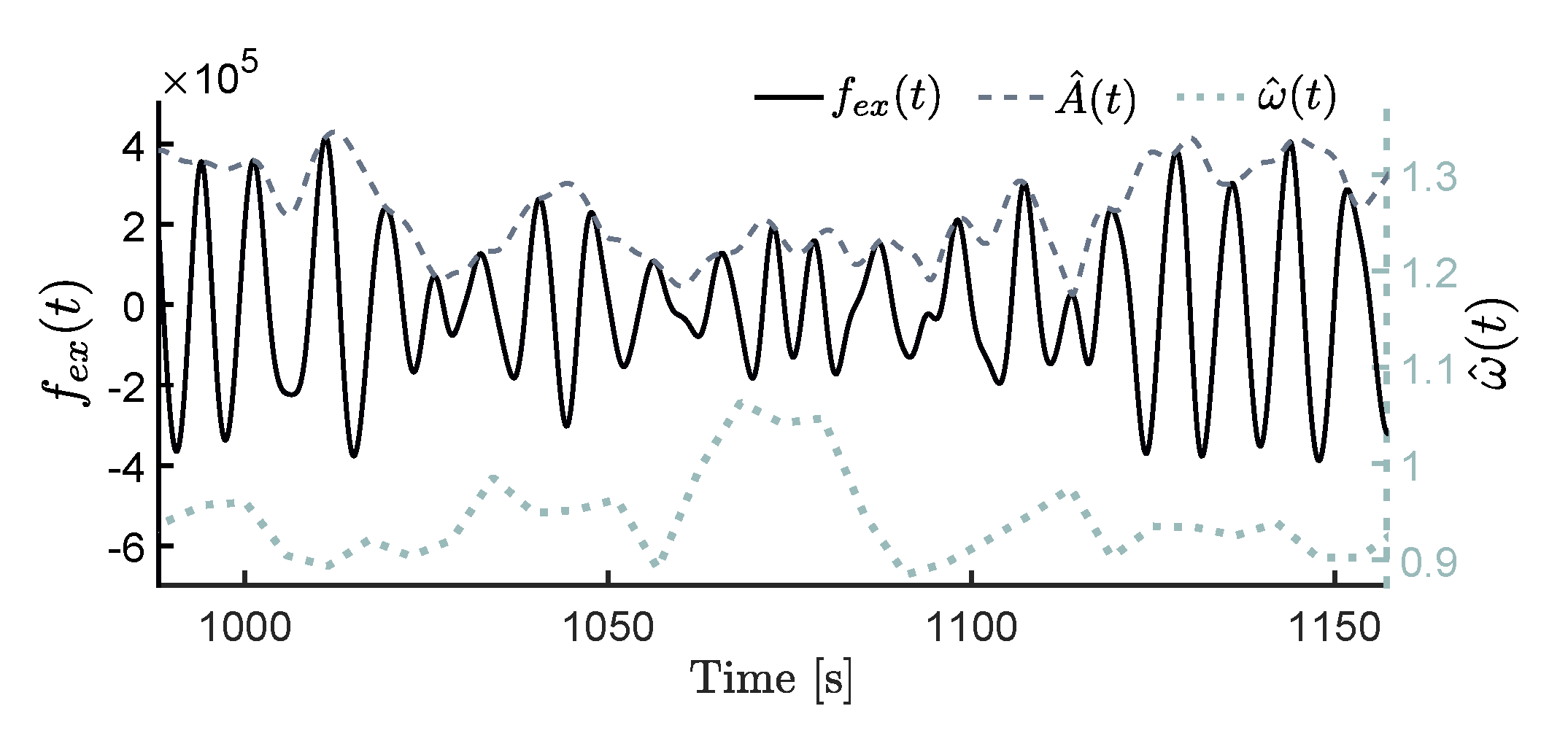
The main difference between the C2 controller and its predecessor (i.e., the C1 controller) lies in the generation of the velocity profile, and its subsequent impact in final energy absorption. In the case of the C2 controller, the reference profile is generated in terms of instantaneous estimates of frequency and amplitude of the wave excitation force signal, computed by means of an EKF strategy. By way of example, Figure 11 shows estimation results for instantaneous amplitude $\widehat{A}\left(t\right)$ (left axis—dashed) and frequency $\widehat{\omega }\left(t\right)$ (right axis—dotted), for a particular sea-state realisation (left axis—solid), with $T_p=8.5$ s.

Note that the sea states that are selected for this case study (see Figure 8) are based on a JONSWAP description with a peak enhancement factor of $\gamma =3.3$, i.e., they are relatively narrowbanded. C2 generally performs better in narrowbanded seas, where a dominant frequency is present, as discussed in Section 4.2. However, and beyond the scope of this case study, the reader is reminded that this assumption might not always be fulfilled in a practical scenario. See Section 4.2 for further discussion.

5.1.3. C3

The design of this feedback controller begins with the definition of a finite set of frequencies $\mathsf{\Omega }$, as detailed in Equation (24), which allows for the computation of an approximation of the device velocity in terms of a finite set of frequency components (see Equation (26)). Such a set $\mathsf{\Omega }$ can be empirically defined, by explicitly using the frequency-domain characterisation of the stochastic process describing the different sea-states under analysis. In other words, the set $\mathsf{\Omega }$ is generated in order to guarantee a suitable representation of excitation forces with significant frequency components in the range corresponding with $\left[0.3,2\right]$ rad/s, i.e.,

$$\mathsf{\Omega }=\left\{{\omega }_k\in {\mathbb{R}}^{+}\left|{\omega }_k=\frac{\pi }{10}+\frac{(\frac{\pi }{2}-\frac{\pi }{10})}{63}k,k\in \{0,\dots ,63\}\right.\right\},$$

(40)

which represents a set with a cardinality of 64.

Subsequently, to determine estimates of each $A_i$ and ${\varphi }_i$, in Equation (26), different FFT windows lengths, which are empirically determined using an exhaustive search methodology, are used for each different considered sea-state. In addition, each controller $K_i^{C3}\left(s\right)$ (see Equation (29)) is tuned, so that energy-maximisation is achieved, at each ${\omega }_i$, while bearing in mind closed-loop stability. Thus, from a dynamical systems point of view, the resulting set ${\mathbf{K}}^{C3}$, considering the cardinality of the set $\mathsf{\Omega }$, represents a diagonal system of order 64.

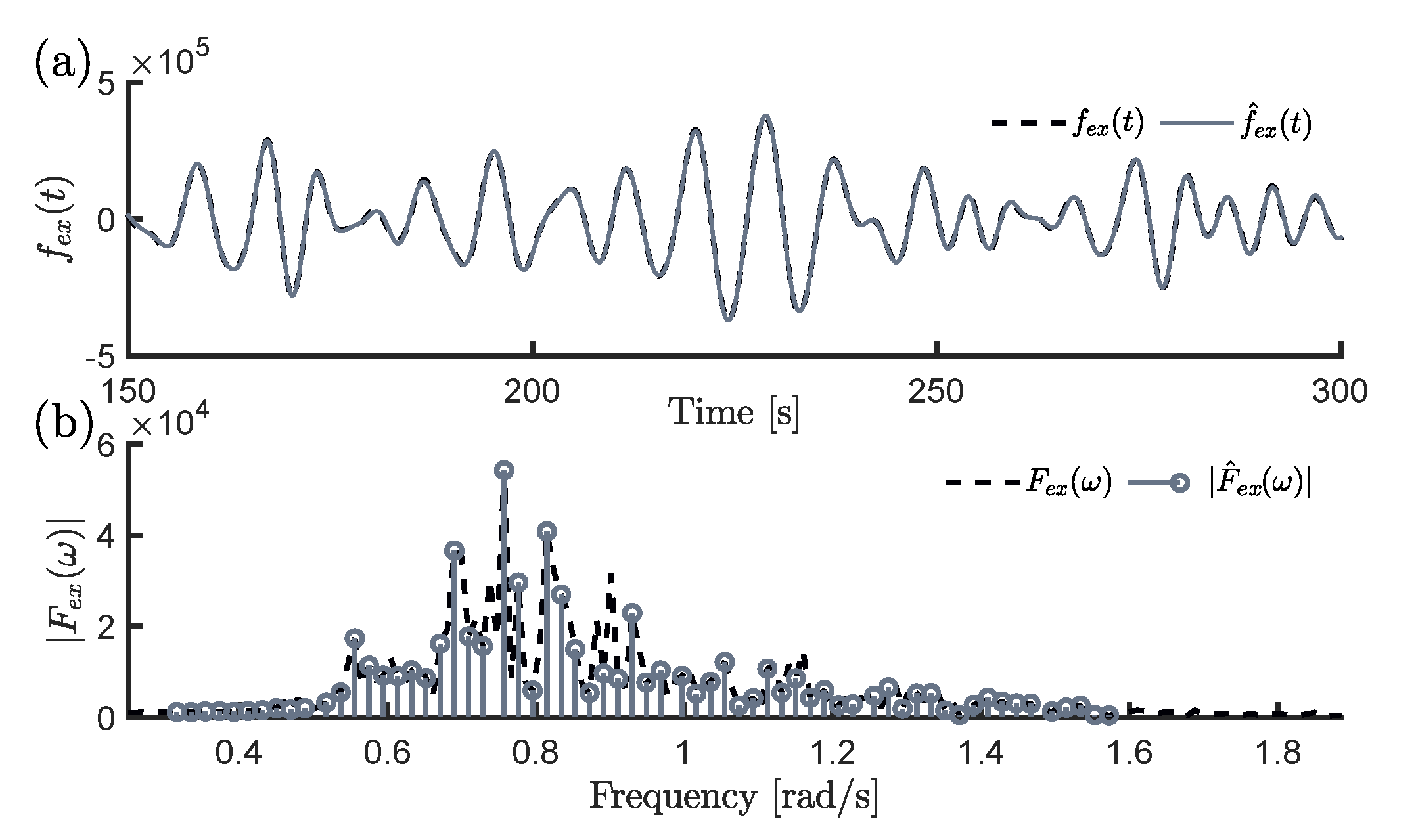
By way of example, when considering the assumption expressed in Equation (25), which essentially inspires this control strategy, Figure 12a illustrates the approximation ${\widehat{f}}_{ex}\left(t\right)$ (dashed line) obtained with the associated set of finite frequencies that are described in (40), for one particular realisation of the excitation force $f_{ex}\left(t\right)$ (solid line), computed according to a stochastic description with $T_p=8.5$ s. Furthermore, Figure 12b provides the spectral representation of each of the excitation force time-traces, i.e., ${\widehat{f}}_{ex}\left(t\right)$ and $f_{ex}\left(t\right)$, using dashed and solid lines, respectively.

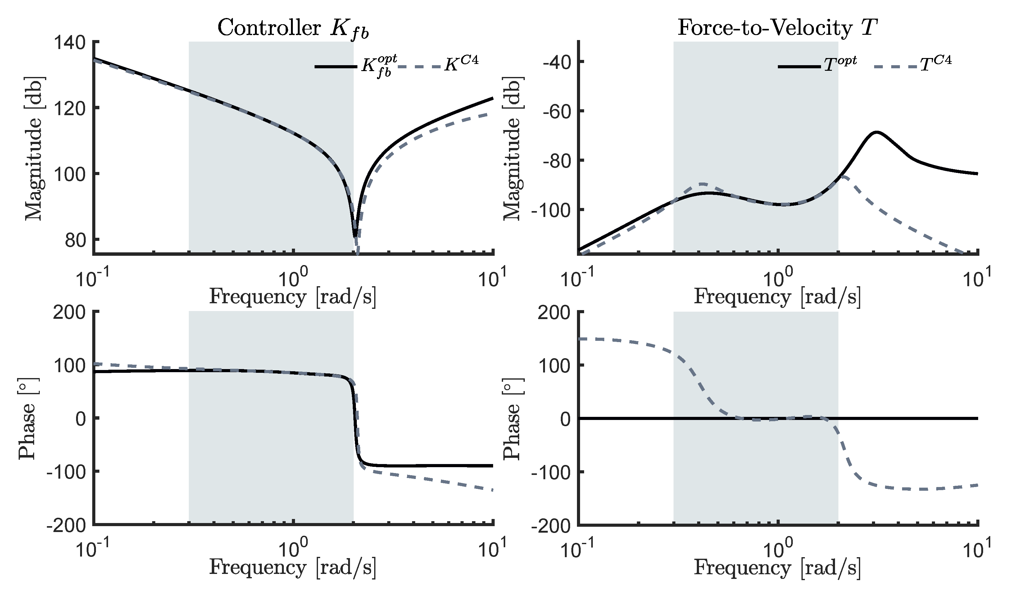
5.1.4. C4

The C4 control strategy, as depicted in Figure 5 and expressed in Equation (31), is essentially based on the application of system identification routines, considering a feedback control structure, as mentioned in Section 4.4. In order to satisfy Equation (31), frequency domain-based system identification routines are applied in this study. In particular, traditional least-mean-square error minimisation algorithms, for transfer function structures, are considered8. The identification process, required to compute $K^{C4}$, is performed using the data set defined for $K_{fb}^{opt}$ in Equation (10), which is essentially based on the WEC frequency-response mapping $G_0$. The resulting controller, for the CorPower-like device that was considered in this case study, is given by the expression

$$K^{C4}\left(s\right)=\frac{-1.195\times {10}^6{s}^2+5.883\times {10}^{4}s-5.244\times {10}^6}{s^2+9.800s+0.216}.$$

(41)

Note that the focus of the frequency-domain identification algorithm is on ensuring the controller approximation in the frequency range characterising the wave inputs, i.e., $[0.3,2]$ rad/s. To be precise, the following relation

$$K^{C4}\left(\omega \right)\approx K_{fb}^{opt}\left(\omega \right),\forall \omega \in \left[0.3,2\right],$$

(42)

holds. This can be clearly appreciated in Figure 13, where the frequency-response mappings, which are associated with the control-loop featuring the approximating structure $K^{C4}$, are explicitly shown. In particular, the left column of Figure 13 shows $K^{C4}\left(\omega \right)$, together with the frequency-response associated with the (theoretical) optimal feedback controller $K_{fb}^{opt}$. In addition, the right column of Figure 13 depicts the input-output frequency-response mapping when the approximating feedback controller $K^{C4}$ is considered, i.e., $T^{C4}\left(\omega \right)$, along with the corresponding (theoretical) optimal input-output frequency-response $T^{opt}\left(\omega \right)$.

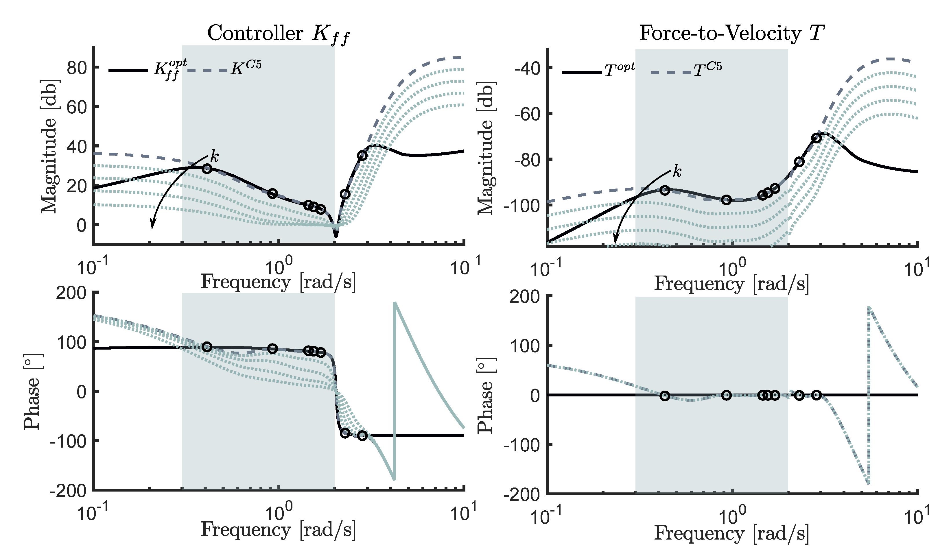
5.1.5. C5

The C5 control strategy, as outlined in Section 4.5, is similar to that of the C4 controller, in the sense that both strategies are essentially based on performing system identification routines, aiming to approximate pre-defined optimal frequency-response mappings. However, there is one fundamental difference: While the C4 control methodology approximates a feedback structure, the C5 control strategy proposes a feedforward equivalent, which allows for constraint handling to be accommodated in a relatively straightforward manner. In particular, the C5 controller $K^{C5}$ aims to approximate the impedance-matching condition that is expressed in Equation (33), i.e.,

$$K^{C5}\left(\omega \right)\approx K_{ff}^{opt}\left(\omega \right),\forall \omega \in \left[0.3,2\right],$$

(43)

where, once again, the focus for the frequency-domain identification algorithm is put on the frequency range characterising the wave inputs. The identification of the feedforward structure $K_{ff}^{opt}$ is performed using a moment-matching-based identification approach, in order to ensure perfect frequency-response matching at a set of user-selected frequencies, as considered by the authors in [13]. Note that the definition of these matching points is designed to improve the fit between $K^{C5}$ and $K_{ff}^{opt}$, within the target bandwidth defined in Equation (43). According to moment-matching-based identification theory [16], the order of the resulting controller is twice the number of matching points. In this study, seven matching points are considered, selected as

$${\omega }_M=\left\{\begin{array}{ccccccc}0.42,& 0.92,& 1.49,& 1.65,& 1.74,& 2.29,& 2.86\end{array}\right\},$$

(44)

generating an approximating structure $K^{C5}$ of order 14. Figure 14 shows the set of frequency-response mappings that are related to the C5 controller. In particular, the left column of Figure 14 illustrates $K^{C5}\left(\omega \right)$, together with the optimal feedforward mapping $K_{ff}^{opt}\left(\omega \right)$. The right column of Figure 14 depicts the force-to-velocity mapping associated with the C5 controller, i.e., $T^{C5}\left(\omega \right)$, along with the optimal force-to-velocity frequency response $T^{opt}\left(\omega \right)$. Note that both the left and right columns also show the effect of varying the constant gain k, used to handle physical limitations, on each respective frequency-response profile. In particular, values for k in the set $\left\{0.5000,0.2500,0.1250,0.065\right\}$ are considered, while using an arrow to indicate a decrease in k. Finally, the matching points, chosen to achieve moment-matching within the system identification procedure (i.e., the elements of the set (44)), are indicated using circular markers.

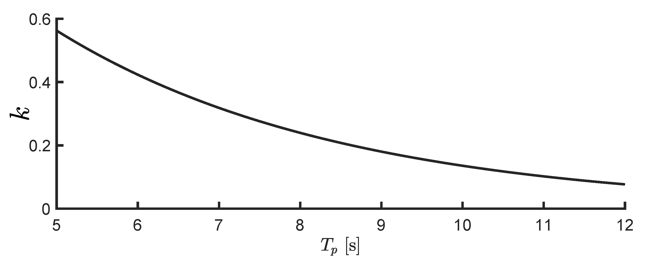
Regarding the tuning of the constraint handling mechanism, for this application case, the value of the constant k (as described in Equations (35) and (36)) is determined using exhaustive (simulation-based) search, depending on each particular sea-state considered. Figure 15 shows the resulting k, for each $T_p\in \left[5,12\right]$ s.

5.2. Performance Analysis: Energy Absorption

In this section, the resulting performance that is obtained which each controller presented in Section 4 is analysed and discussed, for both unconstrained and constrained scenarios. Two performance benchmarks are considered here, as mentioned in the introductory paragraph of Section 5. For the unconstrained case, the theoretical maximum absorbed energy (computed analytically, as in, for instance, [8]), denoted CR1, is considered as a reference measure. In contrast, for the constrained scenario, the performance obtained with an optimisation-based controller, denoted here as CR2, is considered as a surrogate performance reference.

Throughout this section, the performance results for each controller are shown in terms of relative values with respect to each corresponding benchmark case, i.e.,

$$\mathrm{RGP}=\frac{P^C}{P^R},$$

(45)

where RGP denotes the relative absorbed power, $P^C$ represents the power generated with the controller C, i.e., C1, C2, C3, C4, or C5, and $P^R$ denotes the power that is generated with the reference controller R, i.e., CR1 (unconstrained case) or CR2 (constrained case).

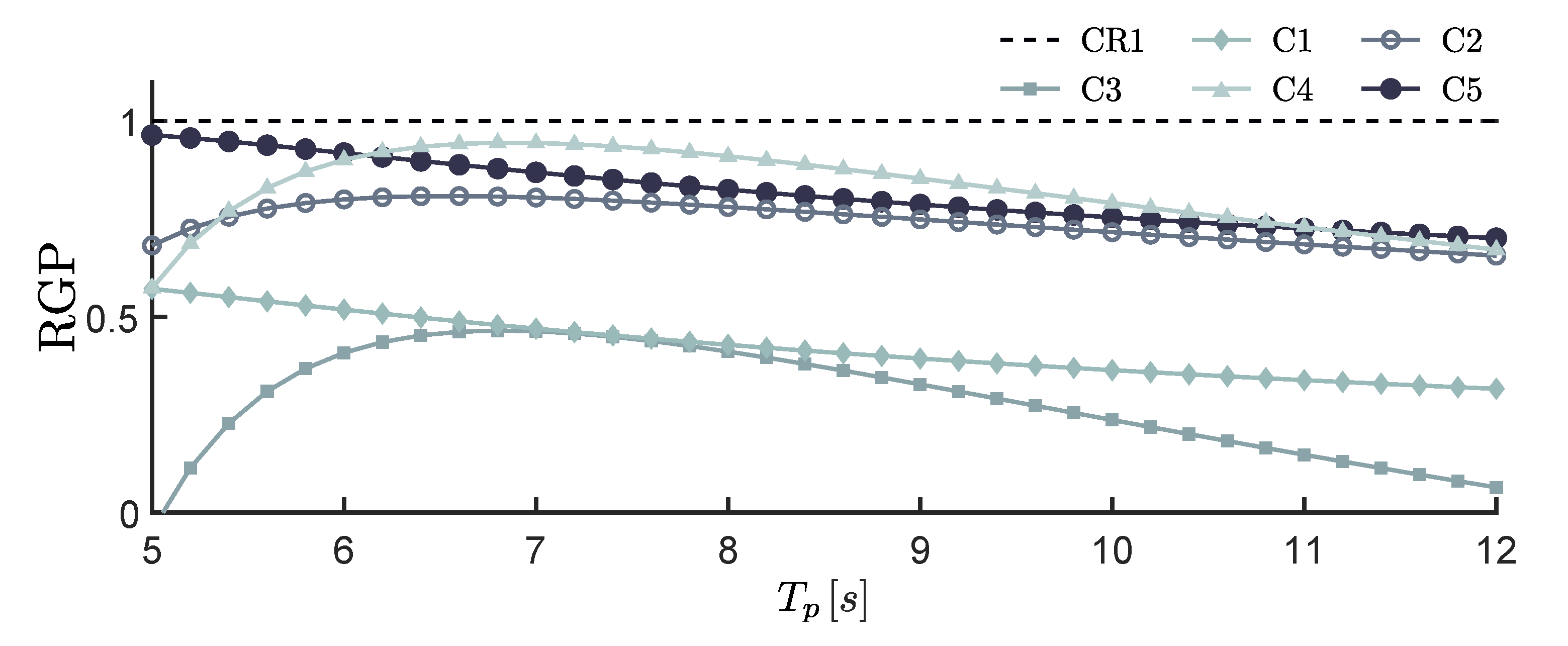
5.2.1. Unconstrained Control

Figure 16 shows performance results in terms of RGP, for the unconstrained case. Note that Figure 16 also includes the maximum relative RGP (dashed-black line), defined as the maximum theoretical achievable energy absorption, i.e., CR1. The RGP values that were obtained with the C1, C2, C3, C4, and C5 strategies, are denoted in Figure 16 using diamond, circle, square, triangular, and dot markers, respectively. It is important to note that, from an overall analysis, it is clear that the C2, C4, and C5 control methods obtain a high performance level, which, in practical terms, is comparable with the maximum achievable RGP. This is especially noteworthy for the case of the C4 controller, which is essentially a simple second-order system. The lowest performance level is obtained with the C3, which achieves its maximum for the central range of $T_p$. However, significant performance degradation can be observed for both lower and higher peak periods.

Note that a significant difference in terms of performance can be appreciated for the only two feedback structures analysed in this study, i.e., C3 and C4. In particular, the C4 controller significantly outperforms the C3 controller, in both terms of power absorption and controller simplicity (i.e., LTI second-order system vs. time-varying control system).

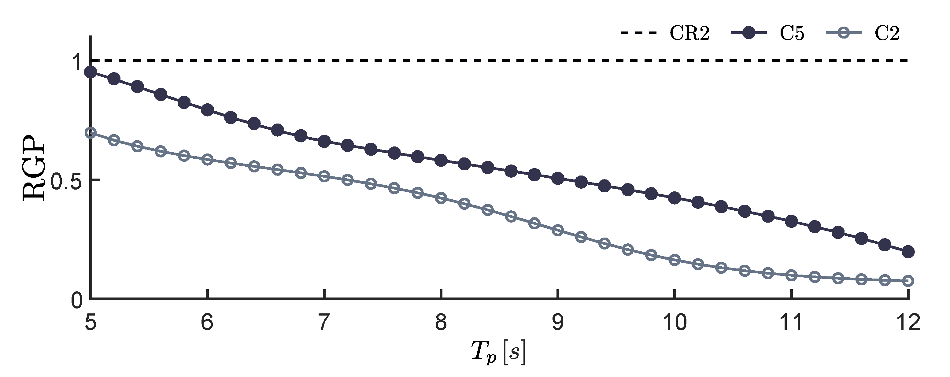
5.2.2. Constrained Control

In accordance with the unconstrained case, as described in Section 5.2.1, the resulting generated power for the constrained scenario is depicted in Figure 17. Analogously to Figure 16, Figure 17 also illustrates the maximum achievable performance, obtained via the surrogate reference measure CR2 (dashed-black line). Note that only the C2 and C5 control methodologies can be considered for performance assessment in the constrained case, since the other control strategies that are presented in Section 4, i.e., C1, C3, and C4, do not provide constraint handling mechanisms. The RGP obtained with the C2 and C5 strategies, is denoted using circle and dot markers, respectively. From an overall analysis, it can noted that, in general, the C5 controller performs better than the C2, for the totality of the analysed peak wave periods. In addition, both of the controllers show decreasing performance with increasing period $T_p$.

In particular, both of the controllers achieve their best performance when short $T_p$ values are considered, i.e., $T_p\approx 5$, since the oscillation amplitude of the considered waves decreases along with $T_p$ (according to the spectrum considered) and, consequently, the displacement constraint is not active. Further discussion on this topic can be found in [32].

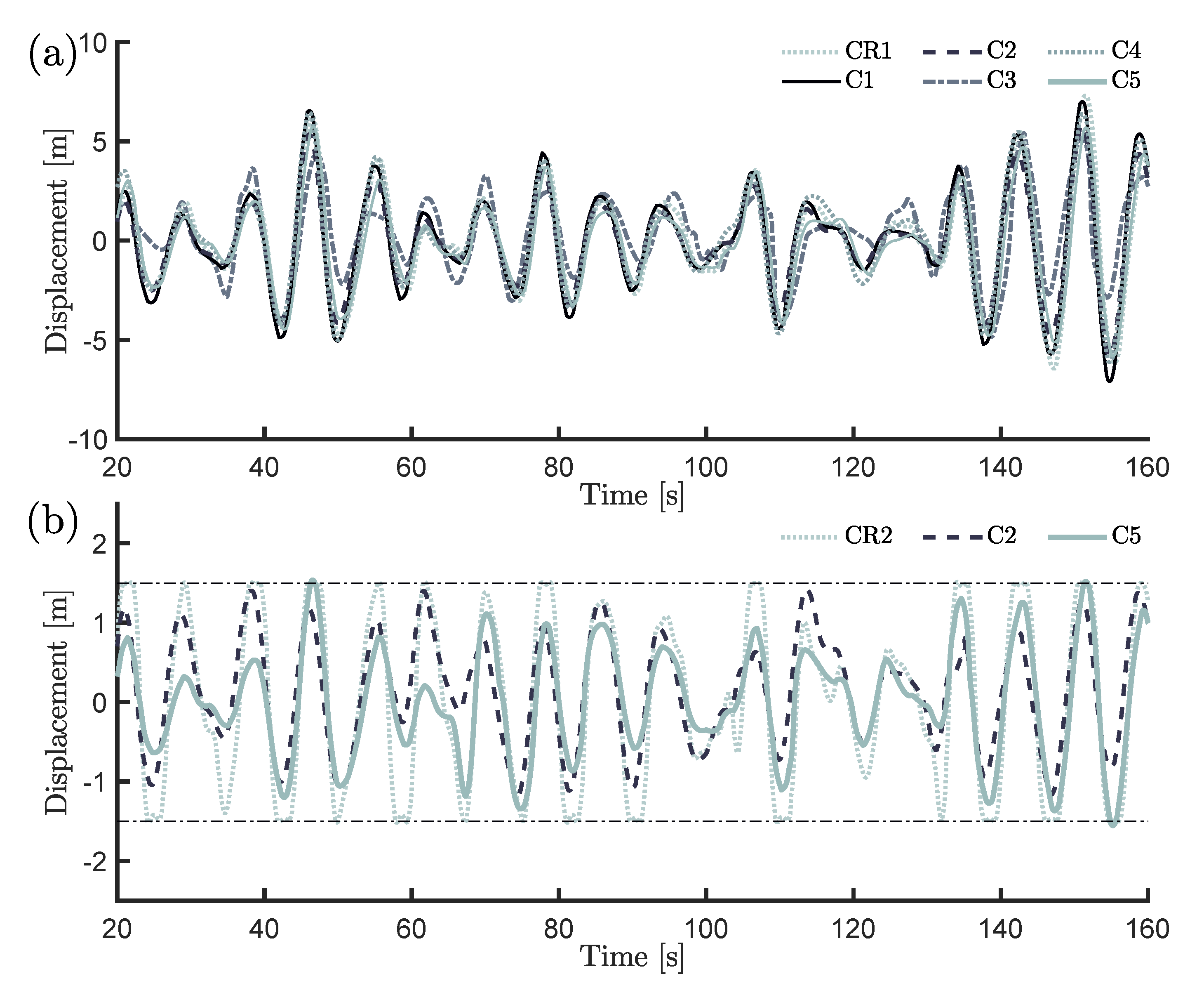
5.3. Time-Domain Response

Figure 18 illustrate a particular set of time-traces obtained with each control strategy studied, for a JONSWAP sea-state (as described in Section 5), with a peak period of $T_p=8.5$ s, for both constrained (a) and unconstrained (b) cases. The results related to each controller, i.e., C1, C2, C3, C4, and C5, are denoted using thick-solid black, dashed, dash-dotted, thick-dotted, and solid-grey lines, respectively. In addition, unconstrained and constrained benchmark references, i.e., CR1 and CR2, are indicated with thin-dotted lines, in Figure 18a,b, respectively.

In the unconstrained case, as shown in Figure 18a, a large deviation with respect to the reference CR1 can be noted for the C3 controller, both in terms of instantaneous amplitude and phase. Note that, the effects that were observed in each corresponding time-domain behaviour, directly support the performance results (in terms of generated power) presented in Figure 16. Finally, in the constrained case, as depicted in Figure 18b, the C5 controller exploits the allowed displacement region more effectively than the C2 controller, which is directly translated into an increase in power production, supporting the results that are presented in Figure 17.

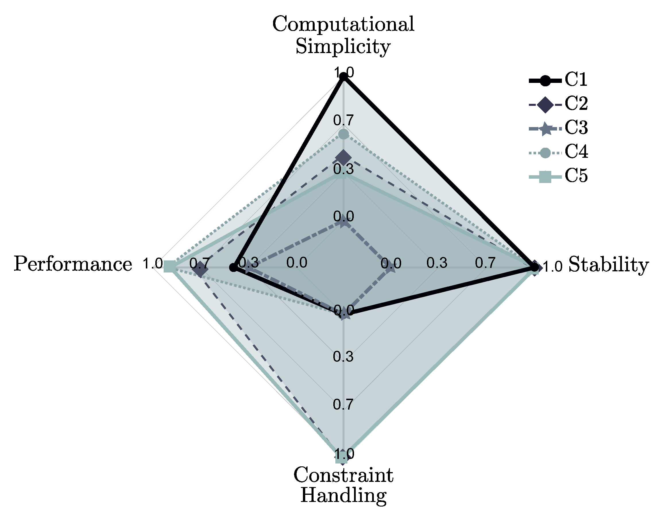
6. Discussion

This section presents a general discussion on the overall controller design procedure, while taking into account both capabilities and energy-maximising performance of each simple control strategy. To this end, this section provides a critical comparison between methods, using four distinguishing features (or categories): (1) computational simplicity; (2) stability; (3) constraint handling capability; and, (4) performance. In particular, a rating system is proposed, aiming to assign a score to each of the above categories, with such a score taking values between 0 (minimum) and 1 (maximum), for each controller analysed in this paper. The underlying principles behind each of this features, and its associated scoring system, are described in the following paragraphs.

• Computational Simplicity. With the aim of analysing computational simplicity,

  Table 3. Normalised run-time and computational simplicity scoring for each controller.

  Controller	Run-Time ${\mathit{t}}_{\mathit{R}}$	Scoring $\mathit{S}\left({\mathit{t}}_{\mathit{R}}\right)$
  C1	$0.2\times {10}^{-3}$	1.00
  C2	$9.8\times {10}^{-3}$	0.46
  C3	$303\times {10}^{-3}$	0.00
  C4	$2.5\times {10}^{-3}$	0.65
  C5	$28\times {10}^{-3}$	0.32

  presents controller normalised run-time (denoted as $t_R$), i.e., ratio between the time required to compute the control signal for each controller, and the length of the simulation itself (in seconds). The computations are performed using Matlab^® R2019a, running on a PC comprising an Intel^® Core™i3-2120 CPU @ 3.30 GHz processor with 16 GB of RAM operated by a Windows 10 Pro 64 bits version 2004 compilation OS 19041.450. Table 3 also presents the corresponding scoring that is assigned to each of the analysed controllers, based on the relation described in the following. Note that, given the wide range of normalised run-times calculated (see Table 3), a normalised logarithmic scale is used for scoring the computational simplicity. Let $t_R^{\min }$ and $t_R^{\max }$ be the minimum and maximum normalised run-times among the set of five controllers. The scoring $S:\mathbb{R}\to [0,1]$, $t_R\mapsto S\left(t_R\right)$, for each controller is defined via:

  $$S\left(t_R\right)=1-\frac{{log}_{10}\left[\frac{t_R}{t_R^{min}}\right]}{{log}_{10}\left[\frac{t_R^{max}}{t_R^{min}}\right]}.$$

  (46)
  It is straightforward to note that $S\left(t_R^{\min }\right)=1$ and $S\left(t_R^{\max }\right)=0$, i.e., in terms of run-time, the slowest controller is rated with 0 (minimum score), while the fastest is scored with 1 (maximum score).
• Stability. It is well-know that stability is a classical issue in controllers based on the energy-maximising impedance-matching principle, as mentioned in Section 4. When considering the discussion provided in Section 4 related to the stability of each controller, this category is rated, as follows:
  • If the stability of the control loop can be fully guaranteed, the controller is rated with 1,
  • if the stability of the control loop cannot be fully guaranteed, the controller is rated with 0.
• Constraint Handling Capability. This category analyses the capabilities of each controller in handling physical limitations, i.e., constraints. In particular, this category is rated as follows:
  • If a controller provides a constraint handling mechanism, the controller is rated with 1,
  • if a controller does not provide a constraint handling mechanism, the controller is rated with 0.
• Performance. Using the performance results that are presented for the unconstrained case (since constrained performance metrics are not available for all controllers), presented in Figure 16, this category measures the total energy-maximising performance with respect to the RGP (defined in Equation (45)), as follows:

  $$\frac{1}{7}{\int }_5^{12}\mathrm{RGP}d{T}_p$$

  (47)

  where the denominator of the quotient, i.e., 7, arises from computing the length (in seconds) of the range of peak periods that are considered to generate the wave inputs. Note that, if the reference measure CR1 is considered, then the expression in Equation (47) is effectively 1.

The results of evaluating each control strategy, following the set of features that are defined above, can be found in both

Table 4. Score assigned to each controller considering each category.

Controller	Computational Simplicity	Stability	Constraint Handling	Performance
C1	1.00	1	0	0.42
C2	0.46	1	1	0.75
C3	0.00	0	0	0.30
C4	0.65	1	0	0.82
C5	0.32	1	1	0.81

, and the four-dimensional spider plot presented in Figure 19.

From the observation of Table 4, Figure 19, and the discussion in Section 4 and Section 5, some comments, related to the status and perspectives of energy-maximising WEC controllers based on the impedance-matching principle, are worth highlighting. Firstly, a strong trade-off between the estimation of wave excitation forces, and capabilities of managing constraints, can be mentioned. In addition, it is noteworthy that, even with a simple feedback structure, high performance levels can be reached, as demonstrated by the C4 controller, which features a second-order LTI system. Nonetheless, the lack of a constraint handling mechanism renders the C4 controller unsuitable for realistic applications, in which large (and potentially unrealistic) displacements may be induced in unconstrained control conditions. This fact, which is also discussed here in Section 3, can be directly appreciated in Figure 18a.

From the analysis of Table 4 and Figure 19, it can be noted that the C5 controller provides a framework in which physical constraints are considered, while, at the same time, good performance levels are effectively achieved. Note that the C2 controller also provides a constraint handling mechanism, via a suitable modification of the feedforward velocity reference generation, although such a mechanism depends upon a nonlinear estimation process. In other words, constraint handling in the C2 has an inherently higher computational (and analytical) complexity than the C5 controller.

The results that are presented in Table 4 and Figure 19 give some clear directions and perspectives for future research and the development of simple controllers for wave energy systems. In particular, there is a clear lack of LTI feedback strategies that are capable of handling physical limitations. Such a scenario, if achievable, would provide controllers capable of optimising energy-absorption by using motion measurements only, dropping any requirement of wave excitation force estimation, while being able to successfully handle constraints. This would be, effectively, an ideal simple controller for WEC systems, completely covering essential requirements for WEC energy maximising controllers.

7. Conclusions and Future Directions

This paper documents a set of (5) controllers, all based on the impedance-matching principle, which have been developed over the period 2010–2020, and compares and contrasts their characteristics, in terms of performance, the handling of physical constraints, dynamical features, and computational load. The comparison is carried out both analytically and numerically, focusing on issues, such as stability, which can arise in the implementation of panchromatic resonant control, and the availability of suitable constraint handling mechanisms, given that the unrealistic motion often required by the impedance-matching condition. The holistic performance of the controllers is assessed under irregular waves in unconstrained, and constrained (where possible), scenarios. The assessment is carried out in terms of relative absorbed power, including a set of benchmark reference performance metrics for each case, and relative computational load.

A scoring system, which considers four specific features, is proposed in this study, aiming to perform a fair comparison between the five controllers. In particular, computational simplicity, stability, constraint handling, and resulting performance, are explicitly taken into account. From this analysis, a number generic limitations can be identified. In particular, as shown and summarised in Section 6, there is an intrinsic link between feedback-based controllers and an inability to handle constraints, while feedforward controllers, able to handle physical constraints, inevitably require wave excitation force estimates, bringing extra computational load and potential sensitivity to excitation force estimation errors.

While this study has some limitations, for example, the relative sensitivity of controllers to modelling error and measurement noise, etc. has not been considered (though the interested reader is referred to [17] in relation to the relative sensitivity of feedforward and feedback controllers), it shows that, for the unconstrained case, low-order LTI controllers can achieve almost theoretical performance levels, in realistic irregular waves. However, to date, there is not a control methodology that provides an estimator-free, low-order structure (i.e. demanding low hardware requirements), while, at the same time, being able to handle physical constraints. This points to an important potential future research direction: the development of an alternative simple, estimator-free, feedback controller, incorporating a suitable constraint handling mechanism. Whether such a controller is possible, given the generic limitations of the set of controllers studies in this paper, remains an open question.