A Useful Manufacturing Guide for Rotary Piercing Seamless Pipe by ALE Method

Abstract

The development of numerical simulations is potentially useful in predicting the most suitable manufacturing processes and ultimately improving product quality. Seamless pipes are manufactured by a rotary piercing process in which round billets (workpiece) are fed between two rolls and pierced by a stationary plug. During this process, the material undergoes severe deformation which renders it impractical to be modelled and analysed with conventional finite element methods. In this paper, three-dimensional numerical simulations of the piercing process are performed with an arbitrary Lagrangian–Eulerian (ALE) formulation in LS-DYNA software. Details about the material model as well as the elements’ formulations are elaborated here, and mesh sensitivity analysis was performed. The results of the numerical simulations are in good agreement with experimental data found in the literature and the validity of the analysis method is confirmed. The effects of varying workpiece velocity, process temperature, and wall thickness on the maximum stress levels of the product material/pipes are investigated by performing simulations of sixty scenarios. Three-dimensional surface plots are generated which can be utilized to predict the maximum stress value at any given combination of the three parameters.

1. Introduction

Metal pipes are categorized into welded pipes and seamless pipes. Welded pipes are commonly manufactured by bending and welding metal sheets, while seamless pipes are produced using the rotary piercing process. It is well recognized that seamless pipe provides more benefits than welded pipe, such as (1) increased pressure ratings; (2) uniformity of geometry, material properties, and matter; and (3) structural strength and fatigue capacities under load. Offshore industry especially requires over 30–40 years of design life and robust design of the piping system, pipeline, and riser structures are requested by adopting reliable materials, manufacturing processes, installation, and operation. Many benefits of seamless pipe, i.e., uniformity of shape and fatigue and strength capacity, allow for higher safety during the operation period of offshore pipeline [1,2,3] and riser structures [4,5,6] from repeated environmental loadings [7,8].

In the rotary piercing process, a heated round billet is fed into a plug by the action of two skewed rolls which rotate in the same direction. The rolls are tilted and placed on opposite sides of the workpiece, providing both rotation and translation to the workpiece. As mentioned by Komori [9], the rolls can be barrel-shaped or cone-shaped. Since the invention of the piercing process over a century ago, numerous empirical and analytical studies have been conducted and one of the good reviews have been conducted by Komori and Mizuno [10]. Experimental studies on cone-shaped-type rotary piercing using lead and wax were performed and a comparison was drawn between two-roll and three-roll cone systems. It was shown that the three-roll cone systems are superior to that of two-roll systems by Khudeyer et al. [11]. The effects of varying the feed angle on the shear strain were studied experimentally using hot steel. Hayashi and Yamakawa [12] found that with larger cross angles, the decrease in the circumferential shear strain is more significant. Moon et al. [13] and Sutcliffe and Rayner [14] conducted experimental work on the rolling process using modelling clay (Plasticine) due to the similarities of its stress–strain behaviour with that of metals and because of its malleability and low cost.

Finite element analysis (FEA) of metal forming processes was further performed to gather the necessary information to design and control these processes properly. In addition, the number of experimental trials can be minimized through the exploitation of FEA, which would significantly reduce the product development lead time. Moreover, with the decrease of experimental work, the overall development cost of the product would be reduced. Nowadays, the advancement of powerful computer technology enables the numerical simulations to consider various physical phenomena during metal processing which include deformation, heat transfer, phase transformation, and ductile fracture [15,16,17].

A two-dimensional rigid-plastic finite element simulation of rotary piercing was performed by Mori et al. [18]. However, the accuracy of the results was low since generalized plane strain was assumed from the simulation. Three-dimensional rigid-plastic finite element analysis was performed by Komori [9]. The number of the elements was limited, and the mesh was relatively coarse because large amounts of computational time were required. Berazategui et al. [19] used the pseudo-concentrations technique to conduct three-dimensional rigid-viscoplastic finite element simulations and a new algorithm was proposed to describe the contact boundary conditions between the tools and the blank. The algorithm was validated with industrial tests of the barrel-type rotary piercing process. However, the numerical analysis of the process was found to be complicated and the computational cost was rather large. Thus, an alternative simplified method was highly required [10]. Shim et al. [20] used a rigid-thermo-viscoplastic finite element method and conducted simulations with AFDEX 3D software to predict the final shape in better detail. Intelligent re-meshing and tetrahedral elements were used which resulted in increased computational cost. The same method was then used to conduct numerical studies on the Mannesmann effect in the piercing process, as well as to compare between the Diescher’s guiding disk and Stiefel’s guiding shoe [21,22].

Lee et al. [23] presented a novel method for adaptive tetrahedral element generation for precision simulation of moving boundary problems such as bulk metal forming. The effects of using tetrahedral solid elements were investigated in a three-dimensional simulation of the forging process with an AFDEX 3D forging simulator. The predictions of both tetrahedral and standard hexahedral elements were in good agreement with experimental data provided that the remeshing technique is employed by Lee et al. 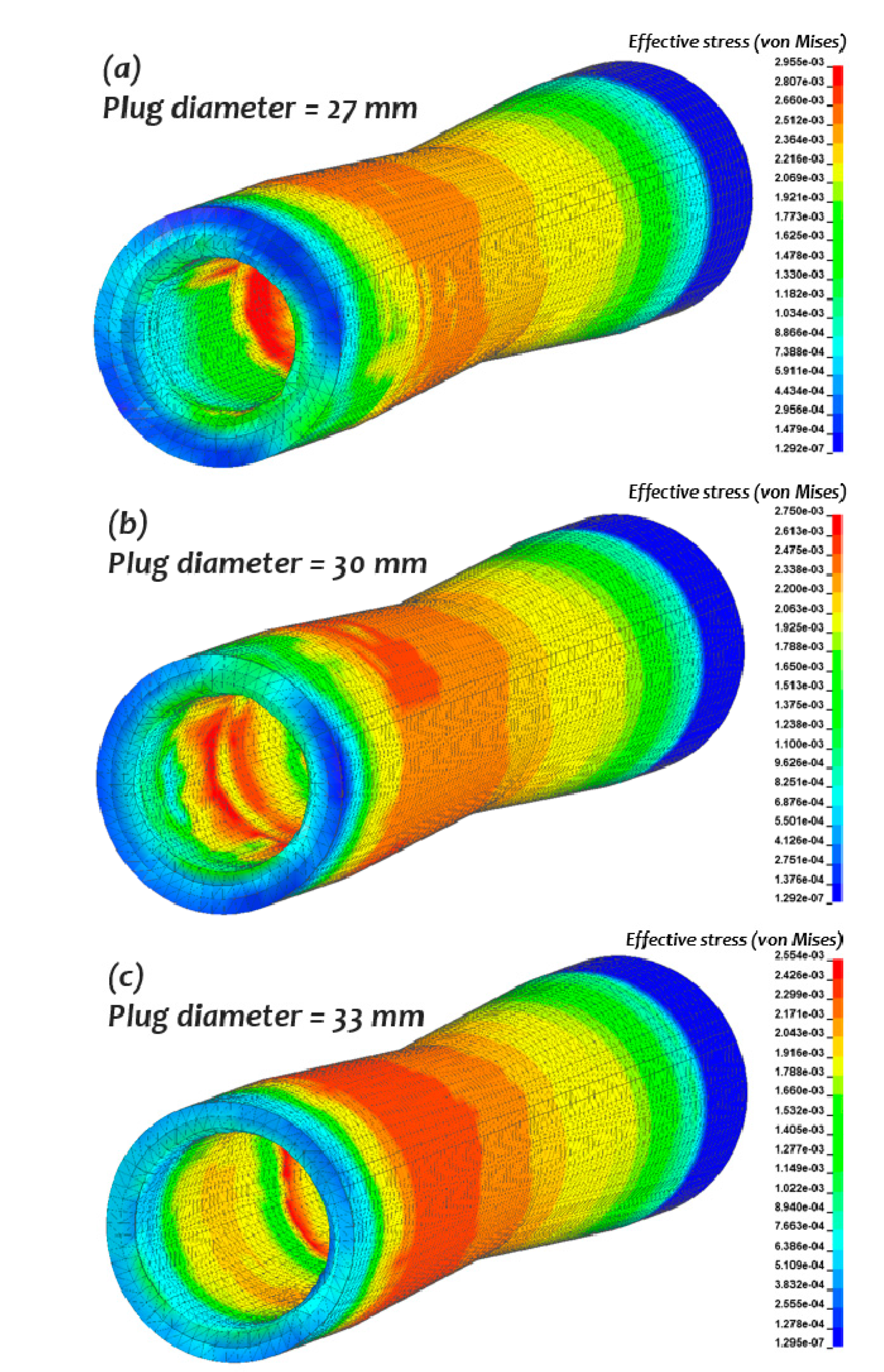[24]. Pater and Kazanacki [25] used Simufact Forming software to analyze the effects of the plug diameter, plug advance, and feed angle on the piercing process. The influence of different plug shapes was further investigated by Skripalenko et al. [26]. ProCAST and QForm commercial software were used for the numerical simulation of piercing aluminium alloy. Jung et al. [27] conducted 3D numerical simulations on the elongation rolling process to study how the rolling speed (rpm) and distance of guide shoes influenced the outer diameter and thickness of the pipe. MSC-SuperForm software was used and an automatic re-meshing method of hexagonal elements was implemented. Xiong et al. [28] used the reproducing kernel particle method for the steady and non-steady analysis of bulk-forming processes and validated the numerical predictions with experimental measurements. Topa and Shah [29] performed 3D numerical simulations for a forging process with a complex tool geometry using the smooth particle hydrodynamics (SPH) method. The results were in fair agreement with experimental data, but the method had a poor visual representation of the final geometry. Hah and Youn [30] presented an effective Eulerian approach for bulk metal forming based on representing boundaries as non-uniform rational B-spline (NURBS) and the effectiveness of the proposed approach was demonstrated by comparing with other numerical methods. However, this approach had the drawback of a blurred boundary condition imposition.

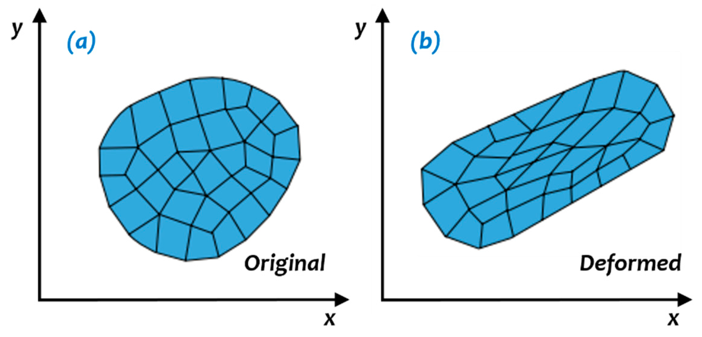
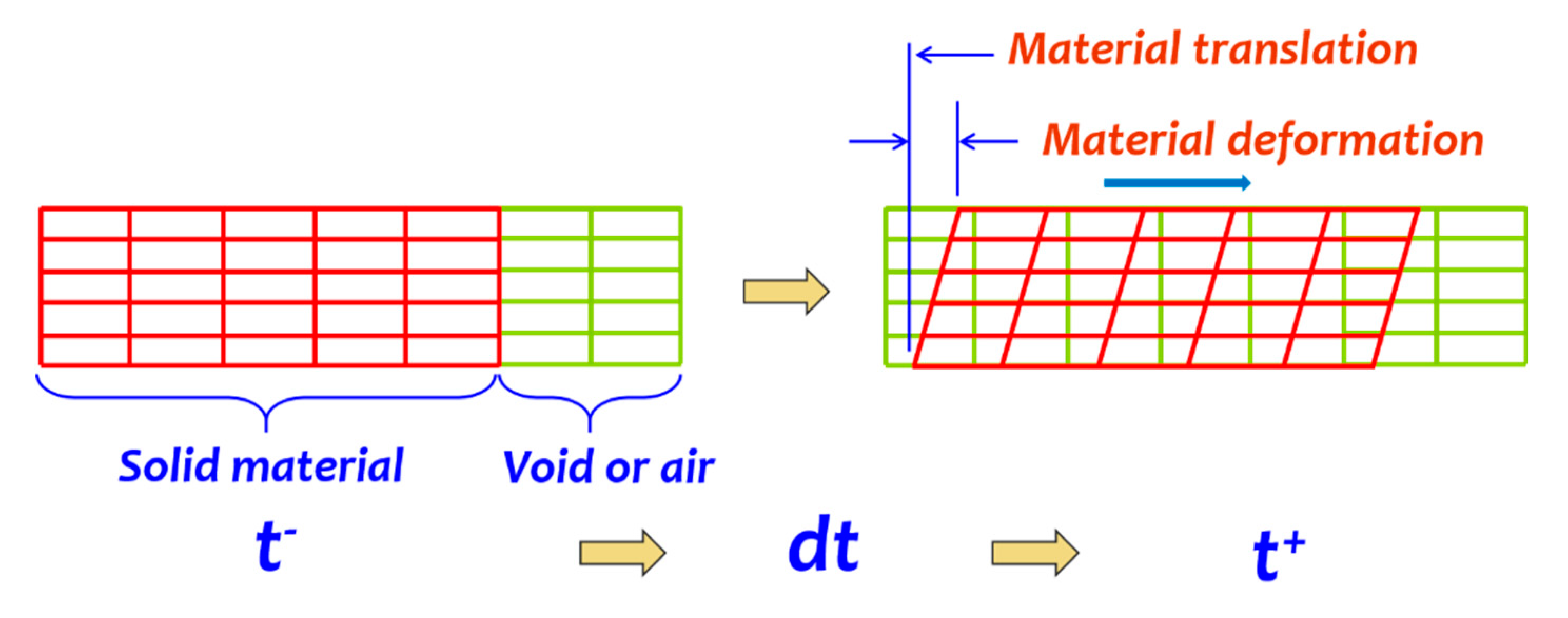
FEA is based on the concept of discretization. A physical structure is divided into a finite number of elements which has a limited number of degrees of freedom. Since the physical structure has an infinite degree of freedom, a discretization error exists. This error can be minimized if the object is discretized into more elements. However, this will increase the computational cost. Another drawback of the conventional finite element method is the limitations in modelling fluid-like behaviour, in which there was excessive deformation of the material. Severe deformation may result in mesh entanglement as illustrated in Figure 1. This limits the material flow and reduces the geometric accuracy of the simulations. Therefore, a new formulation called Arbitrary Lagrangian–Eulerian (ALE) was introduced to solve these challenges. In this formulation, mesh movements and material movements are uncoupled, thus, reducing the elements’ distortion. This formulation was proven to be successful in modelling the fluid-like behaviours of materials during bulk metal forming [31,32,33,34,35].

Vavourakis et al. [36] used a decoupled ALE approach for the extensive deformation modelling of plane-strain elastoplastic problems and the obtained results were validated with limit analysis solutions. The numerical simulations of non-Newtonian fluid flow in a three-dimensional moulding process were performed with the ALE method and the capabilities of this method were demonstrated by Wang and Li [37]. ALE formulations were used for the numerical simulation of a complex continuous-type roll-forming process using the in-house finite element code METAFOR and results were in good agreement with the classical Lagrange method [38]. Recently, the manufacturing chain, including the continuous roll-forming operation, the in-line welding process for closed sections, and the post-cut functions, was numerically simulated with the ALE method by Crutzen et al. [39]. However, validation of the proposed modelling technique was needed as there was no available experimental data in the literature. ALE has proven successful in modelling other areas of metal forming as well. Ducobu et al. [40] adopted the ALE formulation and performed three-dimensional numerical simulations of the orthogonal cutting operation of Ti6Al4V (an alpha-beta titanium alloy with a high strength-to-weight ratio and excellent corrosion resistance). The finite element model was validated against experimental data and recommendations on modelling techniques were proposed. Avevor et al. [41] analysed the chip formation process in the high-speed machining of aluminium alloy AA2024–T351 (a high strength to weight ratio with good fatigue resistance alloy) and utilized the ALE method in the numerical simulations. The predicted cutting forces were compared to those of experimental work and good agreement was found.

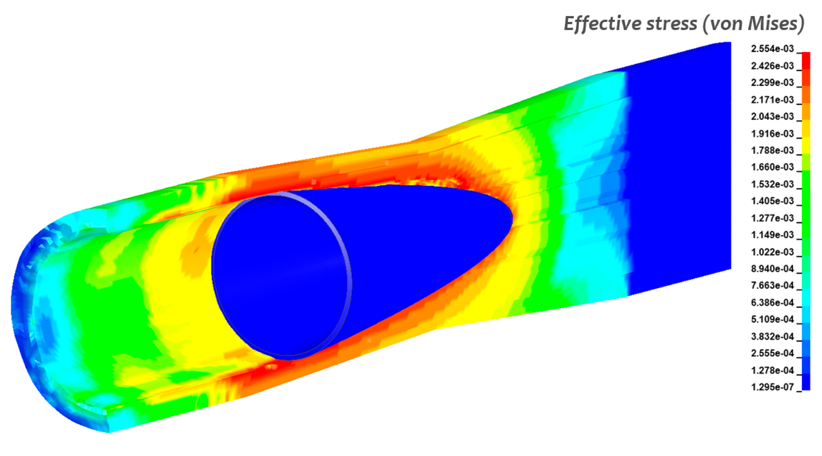
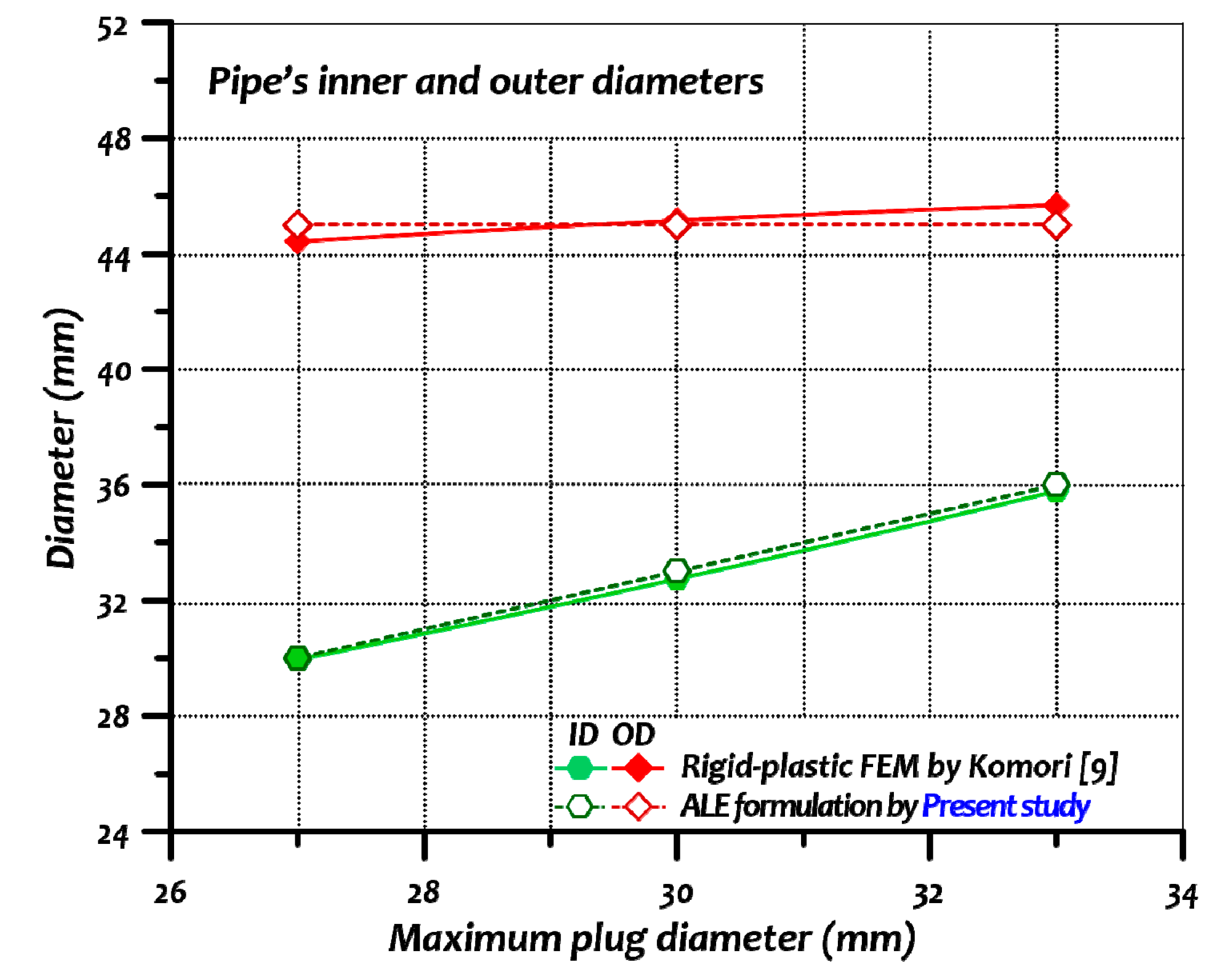
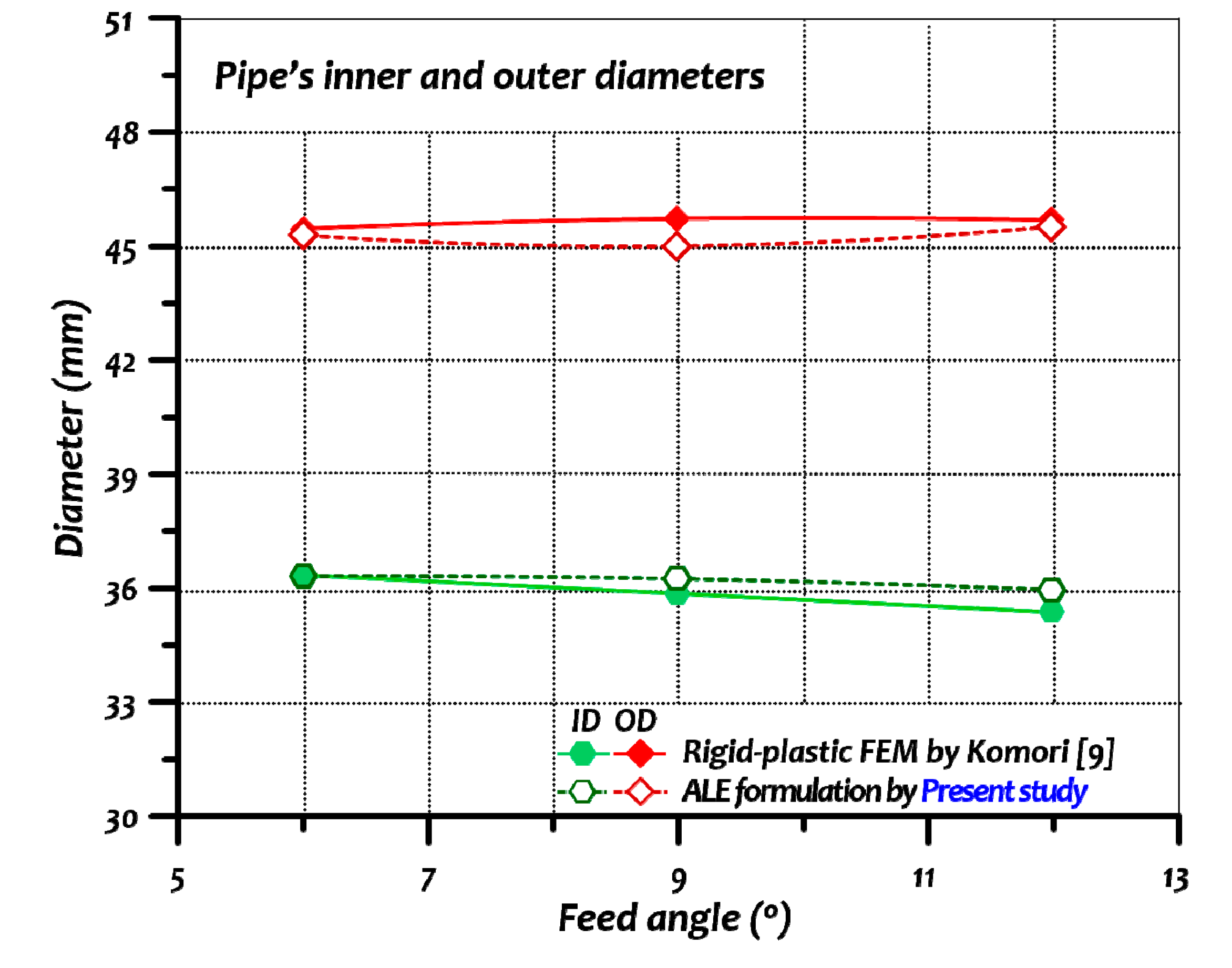
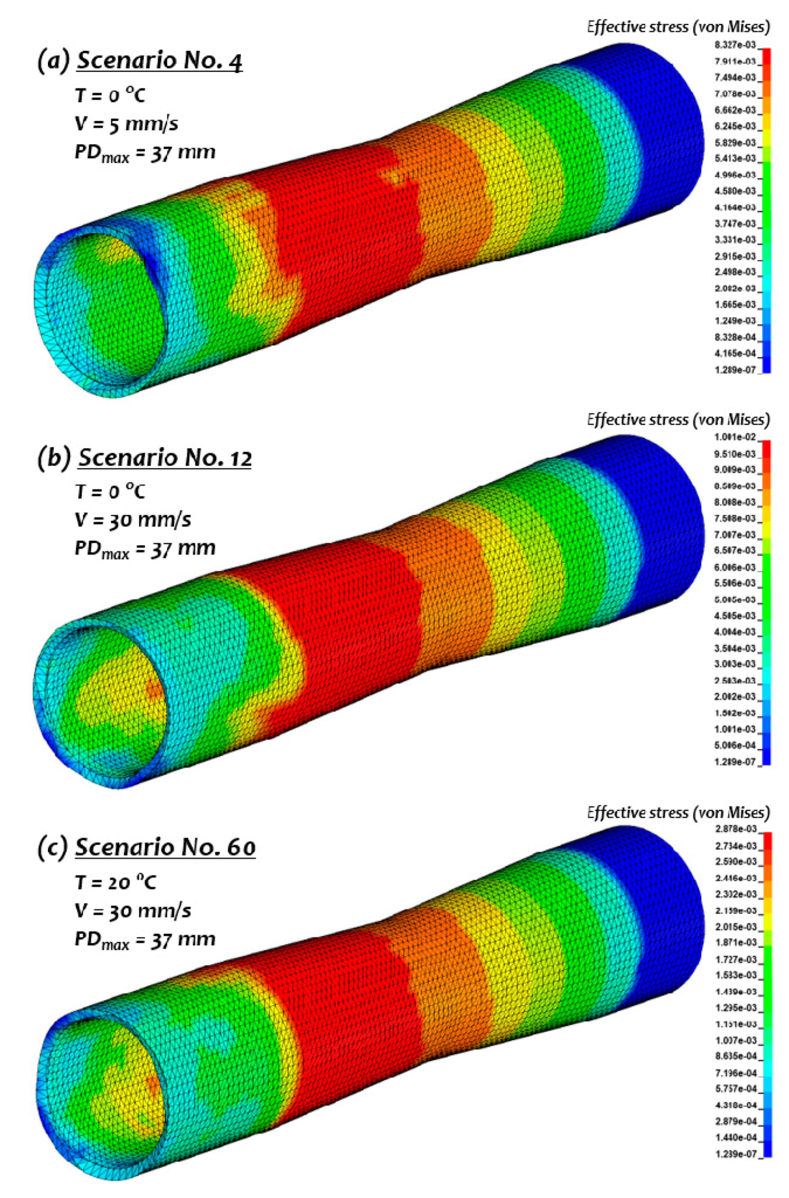
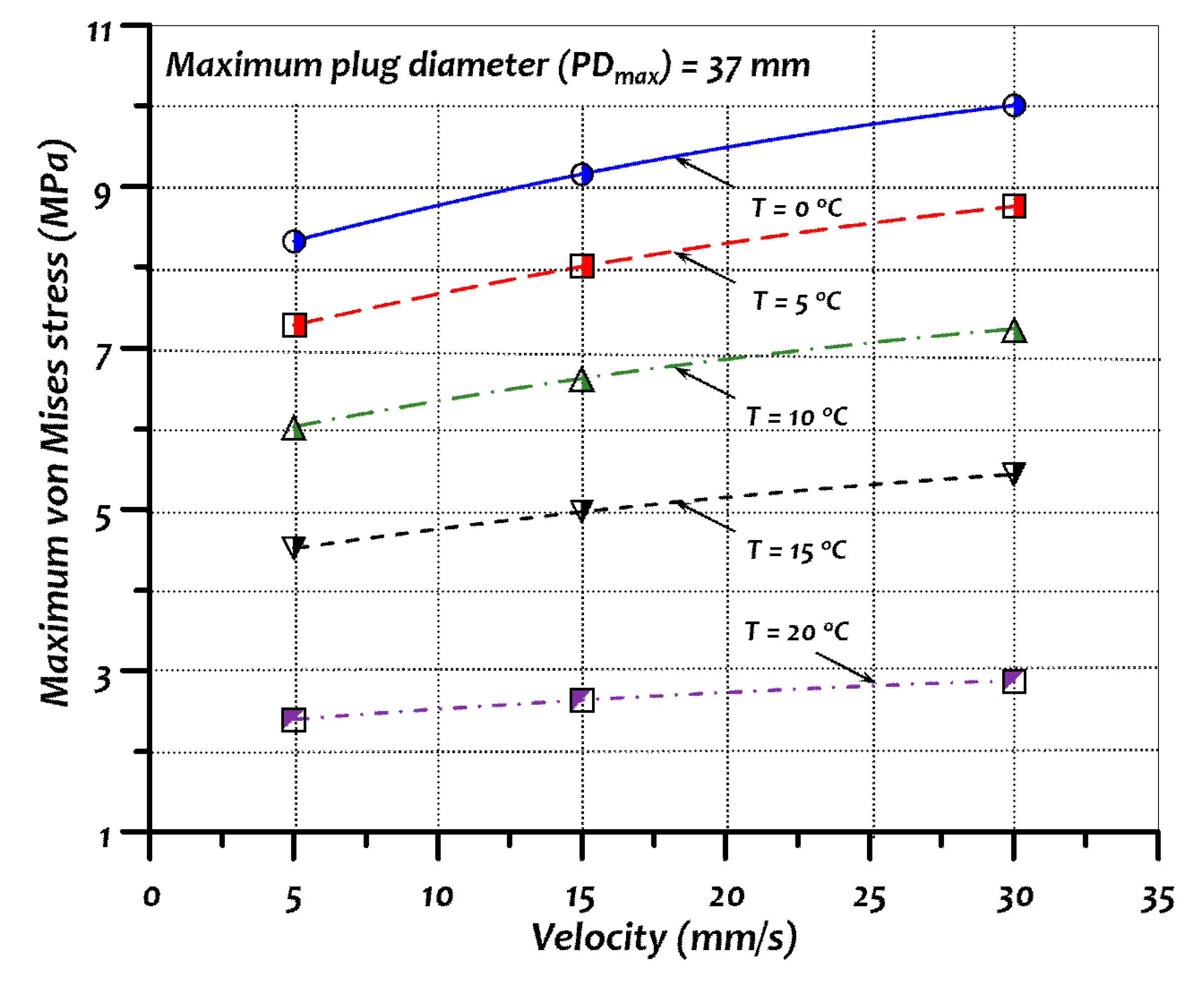
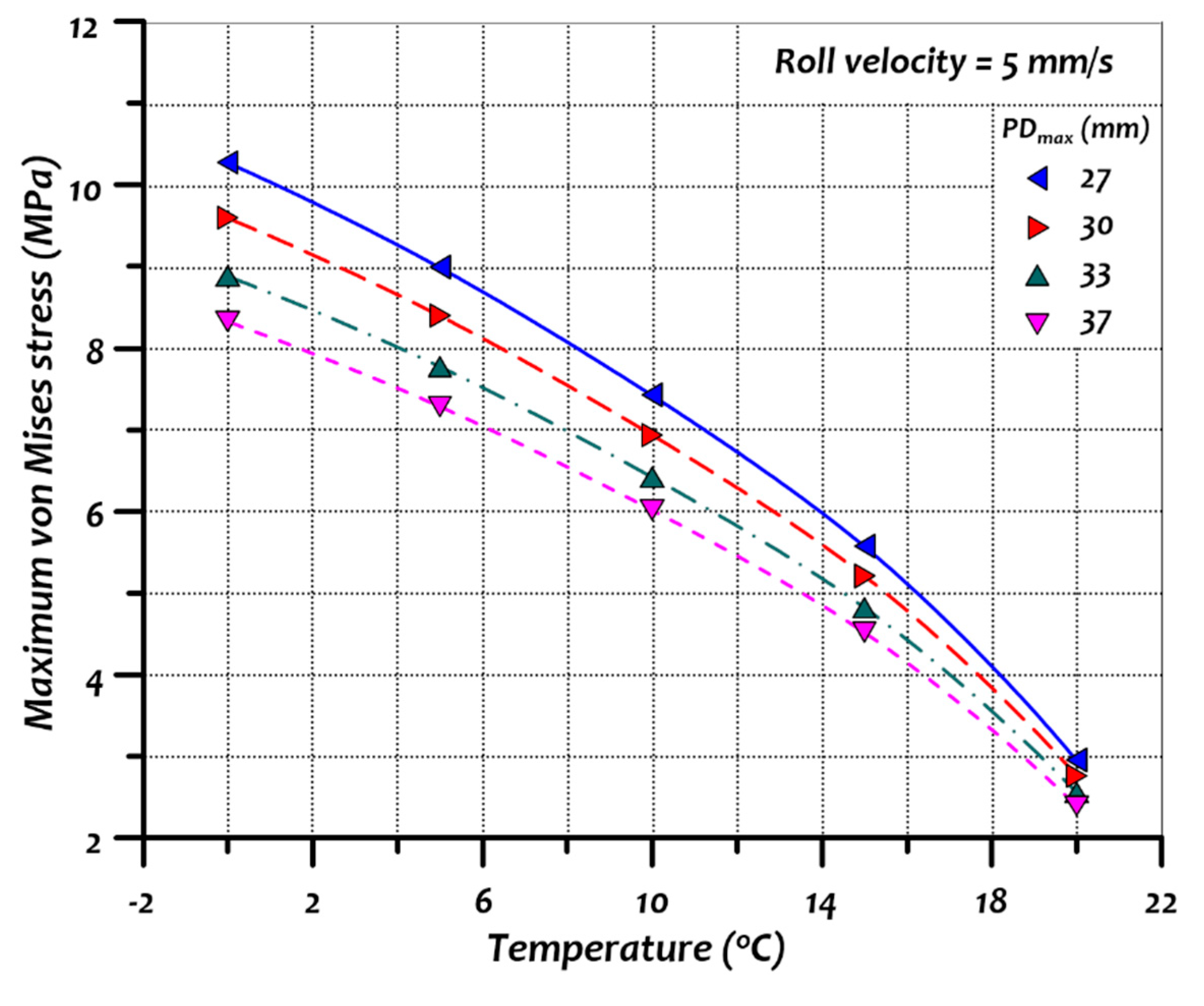
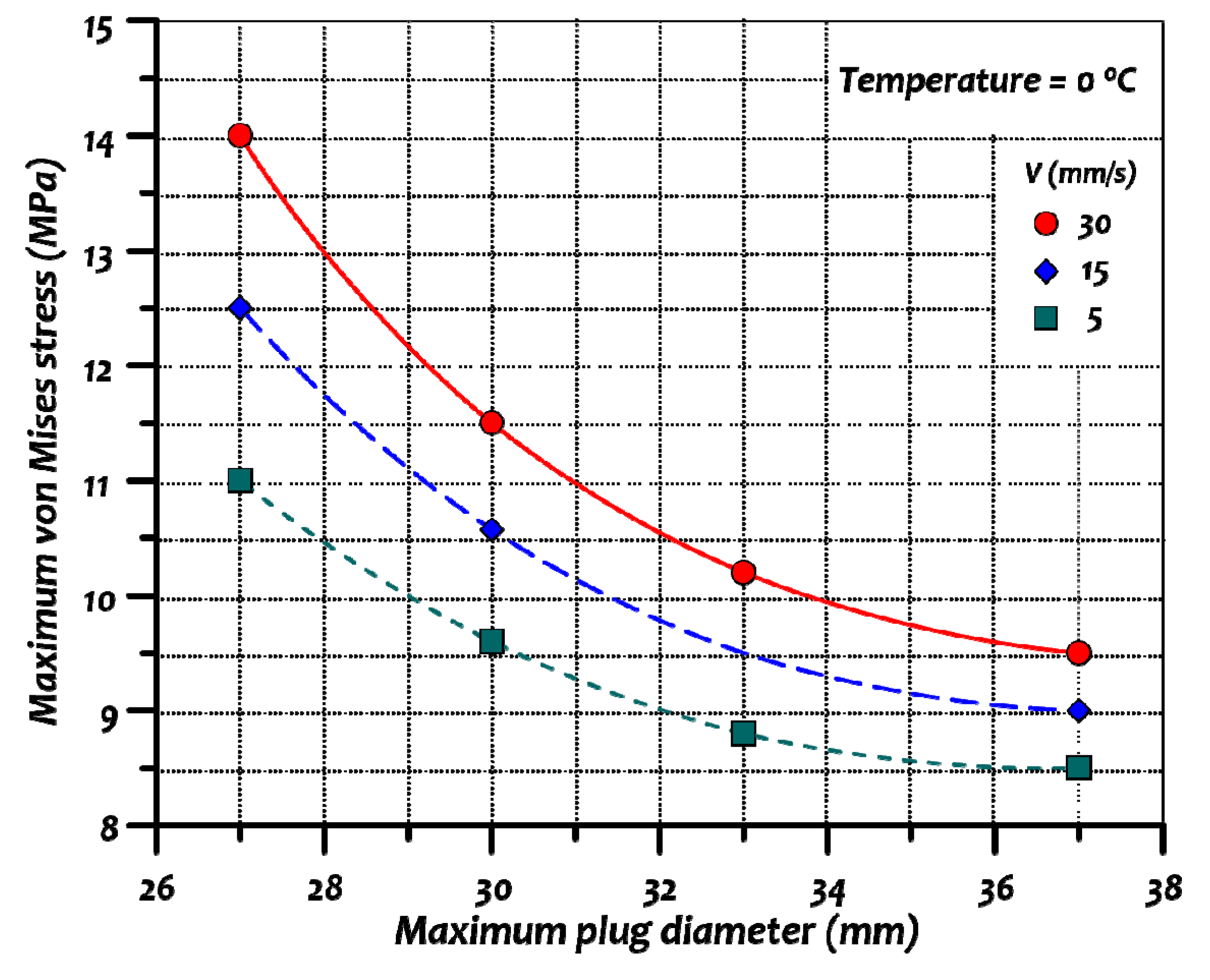
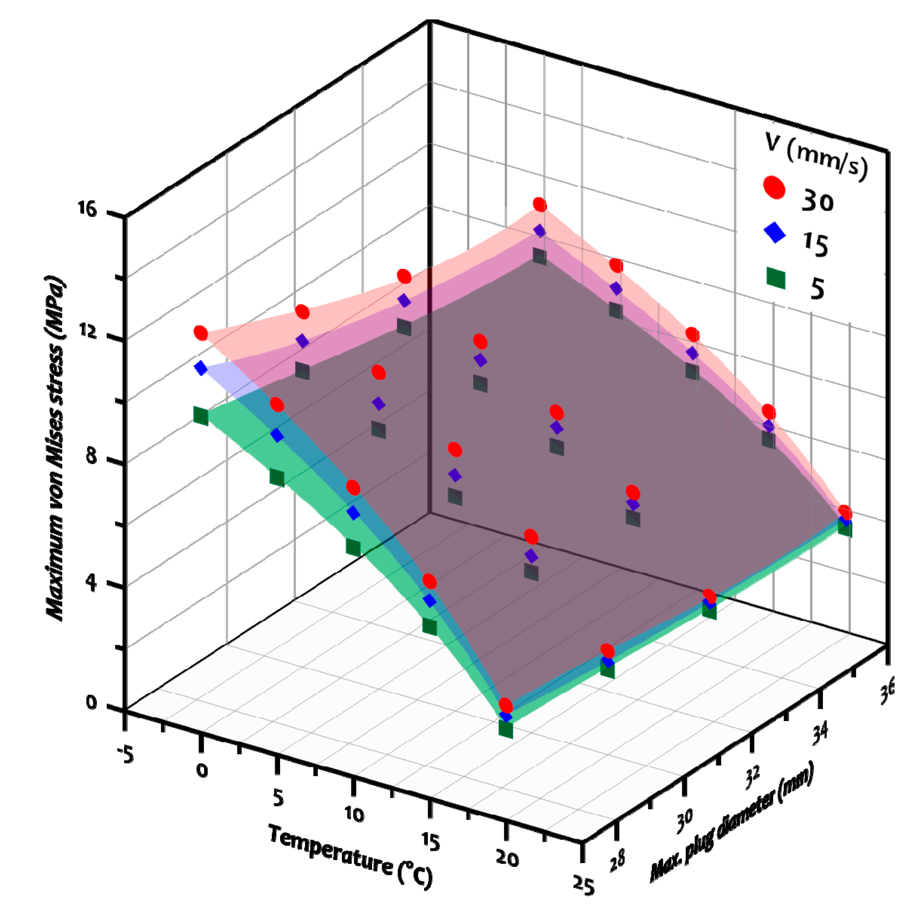
In this paper, the numerical simulations of the rotary piercing process were conducted using an arbitrary Lagrangian–Eulerian formulation with LS-DYNA commercial software [42]. The workpiece used in the experiments has a fluid-like behaviour due to its high workability and large deformation during the piercing process. The results of the numerical simulations were then compared to the empirical data available in the literature [9]. The effects of varying the workpiece velocity, the temperature of the raw material, and pipe thickness on the maximum stress values were investigated.

2. Numerical Simulations of Seamless Pipe Manufacturing Process by ALE Numerical Simulation Method

2.1. Material Models Selection

The stress–strain behaviour of Plasticine is like that of steel in hot conditions, thus, it is a good substitute for modelling the material behaviour during the piercing process. Apart from lead, which is another choice of material, Plasticine is more commonly used due to its low cost and the simplicity of analysing its material kinematics flow during formation [43,44]. The mechanical properties of standard Plasticine were obtained from previous studies [45,46,47], which are listed in

Table 1. Mechanical properties of Plasticine.

Property	Unit	Value
Density	kg/m3	1800
Young’s Modulus	MPa	42.5
Yield Stress	MPa	0.18
Poisson’s ratio	-	0.434

. The stress–strain curves of Plasticine for different strain rates at room temperature are illustrated in Figure 2.

The tools are assumed to be rigid parts as their deformation is insignificant and out of the scope in the current study. They are modelled with shell elements to minimize computational cost. Material model 24 (Piecewise Linear Plasticity) was used to model the Plasticine material behaviour. In this model, the stress–strain curve of the material can be imported to the keyword file to define the relationship between stress and strain. Multiple curves at different strain rates can be used to take into consideration the strain rates’ effects via the stress yield scaling method. Large deformation will cause an increase in the temperature and thermal softening. However, due to the high velocity of the process, it was assumed that changes to temperature were minimal and there was insufficient time for heat transfer to occur between the workpiece and the tools. Thus, the process is simplified to an isothermal system.

The piecewise linear plasticity material model is implemented in steps which are summarized in Figure 3. The pressure, deviatoric stress, and deviatoric strain are expressed as follows, respectively:

$$p=-\frac{1}{3}{\sigma }_{ij}{\delta }_{ij}$$

(1)

$$s_{ij}= {\sigma }_{ij}+p{\delta }_{ij}$$

(2)

$${\dot{\epsilon }}_{ij}^{\prime }= {\dot{\epsilon }}_{ij}-\frac{1}{3}{\dot{\epsilon }}_{ij}{\delta }_{ij}$$

(3)

where ${\sigma }_{ij}$ is the Cauchy stress tensor and ${\dot{\epsilon }}_{ij}$ is the strain rate tensor. ${\delta }_{ij}$ is the Kronecker delta whose value is one when $i=j$ and zero when $i\ne j$. The yield stress is defined as follows:

$${\sigma }_Y=\beta \left[{\sigma }_0+f_h\left({\epsilon }_{eff}^p\right)\right]$$

(4)

where ${\sigma }_0$ is the initial yield stress, $\beta$ the strain rate effects parameter, and $f_h\left({\epsilon }_{eff}^p\right)$ is the hardening function. The hardening function may be specified in tabular form. Otherwise, the hardening will be linear in the form of

$$f_h\left({\epsilon }_{eff}^p\right)=E_p{\epsilon }_{eff}^p$$

(5)

where $E_p$ is the plastic hardening modulus and ${\epsilon }_{eff}^p$ is the effective plastic strain which are given as:

$$E_p=\frac{E_{t}E}{E-E_t}$$

(6)

$${\epsilon }_{eff}^p={\displaystyle \underset{0}{\overset{t}{{\displaystyle \int }}}}\sqrt{\frac{2}{3}{\dot{\epsilon }}_{ij}^p{\dot{\epsilon }}_{ij}^p}dt$$

(7)

In the first step of implementing this material model, the deviatoric stress is elastically updated from $s_{ij}^n$ to $s_{ij}^{n+1}$

$${\overline{s}}_{ij}^{n+1}=s_{ij}^n+s_{ip}{\omega }_{pj}+s_{jp}{\omega }_{pi}+2G{\dot{\epsilon }}_{ij}^{\prime }dt$$

(8)

where the overbar denotes a trial stress value and ${\omega }_{pj}$ denotes the rate of rotation of the neighborhood of P, and $G$ is the shear modulus. Then the von Mises flow rule is checked:

$$\varphi =\frac{1}{2}{s}_{ij} s_{ij}-\frac{{\sigma }_Y{}^2}{3}\le 0$$

(9)

If the condition is satisfied, then the deviatoric stress is accepted. However, if is it violated, then an increment in the effective plastic strain is computed as follows:

$$\Delta {\epsilon }_{eff}^p=\frac{\sqrt{\frac{3}{2}{\overline{s}}_{ij}{\overline{s}}_{ji}}-{\sigma }_Y}{3G+E_p}$$

(10)

where $E_p$ is the current hardening modulus. The trial deviatoric stress is scaled back to the yield surface:

$$s_{ij}^{n+1}=\frac{{\sigma }_y}{\sqrt{\frac{3}{2}{\overline{s}}_{ij}{\overline{s}}_{ji}}}{\overline{s}}_{ij}$$

(11)

This concludes the brief review of the constitutive equations of the piecewise linear plasticity material model. For further details about the theory of plasticity, the reader can refer to references [48,49].

2.2. Workpiece and Tools Geometry

The workpiece is a round billet with an original diameter of 45 mm, which is fed between two tilted coned-shaped rolls with a feed angle of 9 degrees (°) and a constant velocity of 5 mm/s. The rolls have a maximum diameter of 292 mm and the distance between their axes of rotation is 330 mm. Thus, the minimum roll gap is 38 mm. The plug advance is 25 mm and its maximum diameter is 33 mm. These piercing process parameters are listed in

Table 2. Parameters of rotary piercing process.

Parameter	Value	Parameter	Value
Initial workpiece diameter (mm)	45	Distance between roll axes (mm)	330
Minimum roll gap (mm)	38	Feed angle (°)	9
Maximum plug diameter (mm)	33	Entrance face angle (°)	3.5
Plug advance (mm)	25	Exit face angle (°)	3
Guide shoe diameter (mm)	47	Workpiece velocity (mm/s)	5

. These parameters were made identical to those previously reported by Komori [9] for comparison purposes. The schematic diagrams and simulation model of the process are shown in Figure 4 and Figure 5, respectively.

2.3. ALE Keywords and Mesh

In order to use the ALE formulation, the meshes of the initial workpiece geometry and the surrounding space must have merged nodes at their shared boundaries. Solid element formulation 12 was used which stands for 1-point integration element with single material and void. In this element formulation, two overlapping meshes exist. The first is a fixed or movable background mesh while the second mesh is connected to the material which flows through the first mesh. This process can be visualized as two steps. In one step, the material undergoes deformation as in standard finite element methods. In the next step, the element’s state variables such as stress, strain, and velocity are re-mapped or distributed back onto the mesh. Figure 6 is a visualization of material “flowing” in the ALE formulation. As the workpiece was largely deformed during the process, it was modelled with this element formulation and solid hexagonal elements were used.

The interactions (or coupling) between the ALE parts (workpiece) and the Lagrangian parts (tools) are materialized with “Constrained Lagrange In Solid” command. The code will search for the penetrations between the abovementioned parts and apply coupling forces to redistribute the material back into both meshes. A penalty coupling algorithm was used. An improper input of this command will cause leakage problems in which the ALE parts will pass through the tools.

Table 3. Input values for the coupling definition.

Parameter	Description	Value
NQUAD	Number of quadrature points	3
CTYPE	Coupling type	4
DIREC	Coupling direction	2
PFAC	Penalty factor	0.1
FRCMIN	Minimum volume fraction for coupling activation	0.4
ILEAK	Leakage control	2
PLEAK	Leakage control penalty factor	0.1
PFACMM	Mass-based penalty stiffness factor	3

summarizes the input parameters for this command.

2.4. Mesh Sensitivity Study

The accuracy of any FEA analysis depends on many factors including the mesh size. Commonly, a coarse mesh is used in the preliminary stages of the studies in order to get quick results. The finer mesh is used at later stages to obtain more accurate results. However, models with a greater number of elements have higher computational cost. Sensitivity analysis was performed to obtain the optimal mesh size.

Sensitivity analysis was performed for six different mesh sizes. Figure 7 shows the convergence of maximum energy absorbed as the number of elements was increased. Furthermore, the simulations with more than 54,612 elements (average mesh size of 2 mm) resulted in slight changes in the energy absorbed values. By roughly tripling the number of elements to 140,600, only a small change of 3.11% was reported. Therefore, a 2 mm mesh size was selected as the optimum size for subsequent simulations. Figure 8 demonstrates the final obtained result from the process. The chosen mesh size generated a smooth representation of the geometry of the pipe compared to a coarser mesh.

2.5. Results and Validation

The deformation of the workpiece as it is compressed by the rollers and pierced by the plug is shown in Figure 9. This illustrates how the ALE formulation can capture the large deformation of the workpiece. Contour plots of the equivalent von Mises stress in Figure 10 reveal that the maximum stress values are not located on the external surface of the pipe wall, but rather are located near the plug tip. This is due to the stress concentration at this region as the material is being pushed towards the small area of the plug tip. Furthermore, the friction between the workpiece and the plug will contribute to the shearing of the material as it flows tangentially to the plug surface.

Figure 11 shows the volumetric strain contours at different cross-sectional views. It was observed that strain values increased as the material deforms, and the inner diameter became larger. Throughout the process, the strain values were axisymmetric. Investigation of the Lode parameter plot reveals it equals to zero around the area of contact with the plug tip. This state corresponds to a shear stress combined with a hydrostatic stress state which indicates that the material is most susceptible to ductile fracture [51]. Therefore, the plug shape plays an important role in the reliability of the final product.

The results revealed some imperfections in the inner diameter of the pipe. As shown in Figure 12, the final shape is represented by the green solid while the red dotted line indicates a perfect circle. This demonstrated the capability of the ALE method to describe and predict defects in the final shape. Due to these imperfections, different processes are usually required to treat the pipe and improve its dimensions. The outer diameter had no significant imperfections due to the existence of guide shoes which assisted in achieving the final outer diameter.

For validation purposes, the numerical simulations were performed at two additional maximum plug diameters—30 mm and 27 mm—as shown in Figure 13. The average values of the inner and outer diameters were measured in each simulation. Varying the maximum plug diameter affected the inner diameter of the final pipe geometry but had little influence on the outer diameter. Comparisons between the results obtained and experimental data revealed a good positive correlation with a low percentage of error (2.11%) as illustrated in Figure 14. For further validation of the FEA model, additional simulations were performed at different feed angles: 6, 9, and 12 degrees. The variation of the feed angle had an insignificant influence on the pipe’s final dimensions. In all three cases, the results of the final diameters matched well with previous data as shown in Figure 15.

As seen in Figure 13, with smaller plug diameters, the larger final thickness is achieved. For plug values of 33, 30, and 27 mm, the outer diameter to thickness ratios are 7.5, 6.0, and 5.0, respectively. The outer diameter is kept constant throughout this study and the D/t ratio is varied by changing the plug diameter.

3. Sensitivity Analysis by Considering the Effect of Velocity, the Temperature, and the Maximum Plug Diameter

3.1. Selection of Scenarios

The effects of workpiece velocity, material temperature, and maximum plug diameter in different combinations were investigated numerically by performing a total of sixty scenarios. The influence of each variable on the maximum stress values was examined separately by fixing the other two variables. The simulation scenarios were generated by three values of velocity, four values of maximum plug diameter, and five values of material temperature, as listed in

Table 4. Summary of the 60 simulation scenarios.

SN	T	V	PDmax	SN	T	V	PDmax	SN	T	V	PDmax
1	0	5	27	21	5	30	27	41	15	15	27
2	0	5	30	22	5	30	30	42	15	15	30
3	0	5	33	23	5	30	33	43	15	15	33
4	0	5	37	24	5	30	37	44	15	15	37
5	0	15	27	25	10	5	27	45	15	30	27
6	0	15	30	26	10	5	30	46	15	30	30
7	0	15	33	27	10	5	33	47	15	30	33
8	0	15	37	28	10	5	37	48	15	30	37
9	0	30	27	29	10	15	27	49	20	5	27
10	0	30	30	30	10	15	30	50	20	5	30
11	0	30	33	31	10	15	33	51	20	5	33
12	0	30	37	32	10	15	37	52	20	5	37
13	5	5	27	33	10	30	27	53	20	15	27
14	5	5	30	34	10	30	30	54	20	15	30
15	5	5	33	35	10	30	33	55	20	15	33
16	5	5	37	36	10	30	37	56	20	15	37
17	5	15	27	37	15	5	27	57	20	30	27
18	5	15	30	38	15	5	30	58	20	30	30
19	5	15	33	39	15	5	33	59	20	30	33
20	5	15	37	40	15	5	37	60	20	30	37

Note: SN = scenario number, T = material temperature (°C), V = velocity (mm/s), and PD_max = maximum plug diameter (mm).

. The results of the three selected scenarios are illustrated in Figure 16.

3.2. Results and Discussion

It was found that increasing the workpiece velocity resulted in higher stress levels. Referring to Figure 16, the first two results are for scenarios 4 and 12, respectively. In these two cases, all the parameters were identical except for the velocity of the workpiece. At 5 mm/s, the maximum stress was 8.33 MPa while at an increased velocity of 30 mm/s, the maximum stress reached 10.01 MPa. Since the effects of strain rates on Plasticine material are similar to those of steel, the trend of the results shown in Figure 17 can be generalized to the piercing of steel pipes. Data in this figure were generated with the maximum plug diameter constant at 37 mm while the velocity and temperature were varied. The increase of maximum stress values due to the velocity variation at 20 °C was less than 0 °C. Therefore, it can be concluded that the effects of strain rate towards the pipes are more significant at lower temperatures. Preheating the specimen is preferred as it increases the malleability and workability of the material.

Referring again to Figure 16, the middle and last contour plots correspond to scenarios 12 and 60, respectively. The only parameter changed in these two scenarios was the temperature. Increasing the temperature from 0 °C to 20 °C resulted in dropping the maximum stress from 10.01 MPa to 2.88 MPa. This is due to a phenomenon called thermal softening. The general influence of material temperature on the maximum stress values is illustrated by the curves in Figure 18. Each curve represents the maximum stress outcome at a different maximum plug diameter. At higher temperatures, the material becomes softer and more malleable. Therefore, the material provided less resistance to deformation, which in turn yielded lower stress values. It was also observed that the vertical distance between each curve decreased as the temperature rose. Hence, it was concluded that changes in the tool geometry, which was represented by the maximum plug diameter, had fewer effects on the stress values at higher temperatures. Thus, for more complex geometries, it would be preferable to increase the temperature of the workpiece material.

Lastly, the effect of the plug diameter was investigated. The stress contours of three cases are illustrated in Figure 13. With a smaller plug diameter of 27 mm, the maximum stress reached 2.96 MPa, and at a larger plug diameter of 33 mm, the value slightly dropped to 2.54 MPa. It was evident from Figure 19 that increasing the maximum plug diameter resulted in lower stress levels. This was due to the change in the curvature of the plug head. For plugs with smaller diameters, the curvature of its head must be increased. This “sharper” head generates higher stresses towards the workpiece material by pressing against it. Reducing the velocity of the workpiece would marginally help in reducing the stress levels.

Combining the findings from the previous figures, the effects of the three variables on the maximum von Mises stress can be summarized as follows: the increase in temperature and plug diameter resulted in lower stress values while increasing the velocity increased the stresses. A three-dimensional surface plot that depicts the combined effects is illustrated in Figure 20. This plot can be utilized to predict the maximum stress values at any combination of the three primary parameters—material temperature, maximum plug diameter, and workpiece velocity—within the respective limits of each variable considered in this study.

Polynomial fitting equations of the third degree with 10 coefficients were generated for the surface plots as follows:

$$\begin{array}{c}{\sigma }_{von Mises}={\displaystyle {\displaystyle \sum }_{i=0}^3{\displaystyle \sum }_{j=0}^3}{C}_{ij}{x}^i{y}^j, for \left(i+j\right)\le 3\\ =C_{00}+C_{10} x+C_{01} y +C_{11} xy+C_{20} x^2+C_{20} y^2 +C_{21} x^{2}y +C_{12} x{y}^2+C_{30} x^3+C_{03} y^3\end{array}$$

(12)

where $P{D}_{max}$ is the maximum plug diameter (27 ≤ $P{D}_{max}$ ≤ 37), $T$ is the material temperature (0 ≤ $T$ ≤ 20), and C is the coefficient of each term in the equation. The coefficients of each fitting equations and their goodness of fit are listed in

Table 5. Determined coefficients of proposed equation.

Surface	C	Value	C	Value
V = 5 mm/s	C00	−13.45	C11	0.02057
	C10	2.82	C21	−0.0002623
	C01	−0.6224	C12	0.0001563
	C20	−0.1031	C30	0.001158
	C02	−0.003655	C03	−0.0002983
V = 15 mm/s	C00	54.73	C11	0.05132
	C10	−3.005	C21	−0.0007234
	C01	−1.154	C12	0.0002157
	C20	0.06465	C30	−0.0004516
	C02	−0.005454	C03	−0.00033
V = 30 mm/s	C00	−28.33	C11	0.06595
	C10	5.272	C21	−0.0009622
	C01	−1.391	C12	0.0003002
	C20	−0.2039	C30	0.002417
	C02	−0.008803	C03	−0.0003383

and

Table 6. Goodness of fit for each surface plot equation.

Surface	Goodness of Fit	Value
V = 5 mm/s	SSE	0.01303
	R2	0.9999
	Adjusted R2	0.9998
	RMSE	0.0361
V = 15 mm/s	SSE	0.01488
	R2	0.9999
	Adjusted R2	0.9998
	RMSE	0.03585
V = 30 mm/s	SSE	0.4139
	R2	0.9998
	Adjusted R2	0.9995
	RMSE	0.06434

Note: SSE = sum of squared errors, R² = coefficient of determination, and RMSE = root mean square error.

, Figure 21, respectively.

This paper proposes the use of an ALE formulation to perform a three-dimensional finite element analysis of the rotary piercing process of Plasticine material. The capability of the method to describe the large deformation and fluid-like behaviour of the workpiece was shown and the results of the numerical simulations were in good agreement with the experimental data. The validated FEA model was utilized to study the influence of the three main variables consisting of material temperature, maximum plug diameter, and piercing velocity. Three-dimensional surface plots were generated to describe the relationship between the three variables and maximum von Mises stress in the material.

The developed FEA model with ALE formulation gave better results than conventional FEA methods as it does not suffer from the limitations of the latter such as mesh distortion and element entanglement. However, it requires more computational time as it necessitates modelling the surrounding space and, thus, the model will be inherently larger in size. In addition, the interaction between the ALE material and different parts depends on the relative mesh size; inadequate modelling of this coupling will result in a leakage problem which is a widespread problem in modelling with ALE formulations. The optimal parameters for the coupling keyword were obtained through trial and error as it varies from one case to another.

It was found that the piercing velocity has a proportional correlation with the maximum stress values while workpiece temperature and plug diameter have the opposite effect. However, further numerical simulations are necessary if the values of any of the three variables are not within the limited range of this study. These relationships can be generalized to the piercing of the steel due to the resemblance of the stress–strain behaviour of Plasticine to that of steel at elevated temperatures. However, benchmarking analysis with empirical data of the steel piercing process is required.

This work focused on the rotary piercing of Plasticine workpiece materials and failure analysis and crack initiation were not considered. Future work will be to investigate the piercing of a full-scale metal pipe at elevated temperatures. The numerical simulation will then be performed with ALE formulation to predict the critical stress and strain values, which may result in defective products with low structural integrity. Additionally, the ductile fracture criteria may be coupled with the simulation to detect the formation of micro-cracks which cannot be visualized by FEA simulations.

Lastly, seamless pipe is considered one of the well-known solutions to minimize the risks from repeated environmental loadings during installation [52] and operation [53]. From the beginning of the introduction, the advantages of seamless pipe (i.e., increased pressure ratings, uniformity of shape, and structural strength and fatigue under load) were highlighted. Especially, uniformity of geometry and material properties of the seamless pipe may help to reduce the possibility of stress concentration, initial deflection, and welding-induced residual stress [54] which can lead age-related structural damage [55], such as fatigue cracking and its propagation, localized dents [56], corrosion [57,58], and combined corrosion-fatigue [59,60] or corrosion stress and deformation issues [61,62]. In particular, seamless pipe is used for the drilling, rigid-production riser, and small size piping systems by considering fatigue and structural capacities subjected to various types of environmental loadings.

It is believed that this is the right time to investigate how to utilize and maximize the advantages of seamless pipe by resolving manufacturing cost and facility-related issues. The obtained outcomes of this study may help the modelling and production of seamless pipe.

References

1. Yu, S.Y.; Choi, H.S.; Park, K.S.; Kim, Y.T.; Kim, D.K. Advanced procedure for estimation of pipeline embedment on soft clay seabed. Struct. Eng. Mech. 2013, 62, 381–389. [Google Scholar] [CrossRef]
2. Mohd, H.M.; Kim, D.K.; Kim, D.W.; Paik, J.K. A time-variant corrosion wastage model for subsea gas pipelines. Ships Offshore Struct. 2014, 9, 161–176. [Google Scholar] [CrossRef]
3. Yu, S.Y.; Choi, H.S.; Lee, S.K.; Do, C.H.; Kim, D.K. An optimum design of on-bottom stability of offshore pipelines on soft clay. Int. J. Nav. Arch. Ocean Eng. 2017, 5, 598–613. [Google Scholar] [CrossRef] [Green Version]
4. Park, K.S.; Kim, Y.T.; Kim, D.K.; Yu, S.Y.; Choi, H.S. A new method for strake configuration design of steel catenary risers. Ships Offshore Struct. 2016, 11, 385–404. [Google Scholar] [CrossRef]
5. Kim, D.K.; Wong, E.W.C.; Lekkala, M.R. A parametric study on fatigue of a top-tensioned riser subjected to vortex-induced vibrations. Struct. Monit. Maint. 2019, 6, 365–387. [Google Scholar]
6. Kim, D.K.; Incecik, A.; Choi, H.S.; Wong, E.W.C.; Yu, S.Y.; Park, K.S. A simplified method to predict fatigue damage of offshore riser subjected to vortex-induced vibration by adopting current index concept. Ocean Eng. 2018, 157, 401–411. [Google Scholar] [CrossRef]
7. Wong, E.W.C.; Kim, D.K. A simplified method to predict fatigue damage of TTR subjected to short-term VIV using Artificial Neural Network. Adv. Eng. Softw. 2018, 126, 100–109. [Google Scholar] [CrossRef]
8. Kim, D.K.; Wong, E.W.C.; Lee, E.B.; Yu, S.Y.; Kim, Y.T. A method for the empirical formulation of current profile. Ships Offshore Struct. 2018, 14, 176–192. [Google Scholar] [CrossRef] [Green Version]
9. Komori, K. Simulation of Mannesmann piercing process by the three-dimensional rigid-plastic finite element method. Int. J. Mech. Sci. 2005, 47, 1838–1853. [Google Scholar] [CrossRef]
10. Komori, K.; Mizuno, K. Study on plastic deformation in cone-type rotary piercing process using model piercing mill for modeling clay. J. Mater. Process. Technol. 2009, 209, 4994–5001. [Google Scholar] [CrossRef]
11. Khudeyer, W.A.; Barton, D.C.; Blazynski, T.Z. A comparison between macroshear redundancy and loading effects in 2- and 3-roll rotary tube cone piercers. J. Mater. Process. Technol. 1997, 65, 191–202. [Google Scholar] [CrossRef]
12. Hayashi, C.; Yamakawa, T. Influence of feed and cross angle on rotary forging effects and redundant shear deformations in rotary piercing process. ISIJ Int. 1997, 37, 146–152. [Google Scholar] [CrossRef] [Green Version]
13. Moon, Y.H.; Chun, M.S.l.; Yi, J.J.; Kim, J.K. Physical modeling of edge rolling in plate mill with plasticine. Steel Res. 1993, 64, 557–563. [Google Scholar] [CrossRef]
14. Sutcliffe, M.P.F.; Rayner, P.J. Experimental measurements of load and strip profile in thin strip rolling. Int. J. Mech. Sci. 1998, 40, 887–899. [Google Scholar] [CrossRef]
15. Rowe, G.W.; Strugess, C.N.; Hartley, P.; Pillinger, I. Finite-Element Plasticity and Metal Forming Analysis; Cambridge University Press: Cambridge, UK, 1991. [Google Scholar]
16. Hawryluk, M.; Jakubik, J. Analysis of forging defects for selected industrial die forging process. Eng. Fail. Anal. 2016, 59, 396–409. [Google Scholar] [CrossRef]
17. Guo, Z.; Lasne, P.; Saunders, N.; Schillé, J.-P. Introduction of materials modelling into metal forming simulation. Procedia Manuf. 2018, 15, 372–380. [Google Scholar] [CrossRef]
18. Mori, K.; Yoshimura, H.; Osakada, K. Simplified three-dimensional simulation of rotary piercing of seamless pipe by rigid-plastic finite-element method. J. Mater. Process. Technol. 1998, 80–81, 700–706. [Google Scholar] [CrossRef]
19. Berazategui, D.A.; Cavaliere, M.A.; Montelatici, L.; Dvorkin, E.N. On the modelling of complex 3D bulk metal forming processes via the pseudo concentrations technique. Application to the simulation of the Mannesmann piercing process. Int. J. Numer. Methods Eng. 2006, 65, 1113–1144. [Google Scholar] [CrossRef]
20. Shim, S.H.; Cho, J.M.; Lee, M.C.; Joun, M.S. Finite element analysis of a roll piercing process equipped with Diecher’s guiding discs. Trans. Mater. Process. 2012, 21, 19–23. [Google Scholar] [CrossRef] [Green Version]
21. Cho, J.M.; Kim, B.S.; Moon, H.K.; Lee, M.C.; Joun, M.S. Comparative study on Mannesmann roll piercing process between Diescher’s guiding disk and Stiefel’s Guiding Shoe. Inst. Met. Res. 2013, 1532, 843–849. [Google Scholar]
22. Joun, M.S.; Lee, J.; Cho, J.M.; Jeong, S.W.; Moon, H.K. Quantitative study on Mannesmann effect in roll piercing of hollow shaft. Procedia Eng. 2014, 81, 197–202. [Google Scholar] [CrossRef] [Green Version]
23. Lee, M.C.; Joun, M.S.; Lee, J.K. Adaptive tetrahedral element generation and refinement to improve the quality of bulk metal forming simulation. Finite Elem. Anal. Des. 2007, 43, 788–802. [Google Scholar] [CrossRef]
24. Lee, M.C.; Chung, S.H.; Jang, S.M.; Joun, M.S. Three-dimensional simulation of forging using tetrahedral and hexahedral elements. Finite Elem. Anal. Des. 2009, 45, 745–754. [Google Scholar] [CrossRef]
25. Pater, Z.; Kazanecki, J. Complex numerical analysis of the tube forming process using Diescher mill. Arch. Metall. Mater. 2013, 58, 717–724. [Google Scholar] [CrossRef]
26. Skripalenko, M.M.; Bazhenov, V.E.; Romantsev, B.A.; Skripalenko, M.N.; Huy, T.B.; Gladkov, Y.A. Mannesmann piercing of ingots by plugs of different shapes. Mater. Sci. Technol. 2016, 32, 1712–1720. [Google Scholar] [CrossRef]
27. Jung, S.H.; Shin, Y.I.; Song, C.K. Finite element analysis of an elongation rolling process for manufacturing seamless pipes. J. Korean Soc. Precis. Eng. 2014, 31, 923–928. [Google Scholar] [CrossRef]
28. Xiong, S.; Li, C.S.; Rodrigues, J.M.C.; Martins, P.A.F. Steady and non-steady state analysis of bulk forming processes by the reproducing kernel particle method. Finite Elem. Anal. Des. 2005, 41, 599–614. [Google Scholar] [CrossRef]
29. Topa, A.; Shah, Q.H. Numerical simulations of bulk metal forming process with smooth particle hydrodynamics. Aust. J. Basic Appl. Sci. 2014, 8, 198–204. [Google Scholar]
30. Hah, Z.H.; Youn, S.K. Eulerian analysis of bulk metal forming processes based on spline-based meshfree method. Finite Elem. Anal. Des. 2015, 106, 1–15. [Google Scholar] [CrossRef]
31. Schreurs, P.J.G.; Veldpaus, F.E.; Brekelmans, W.M. Simulation of Forming Processes, using the Arbitrary Eulerian-Lagrangian Formulation. Comput. Method Appl. Mech. Eng. 1986, 58, 19–36. [Google Scholar] [CrossRef]
32. Aymone, J.L.F.; Bittencourt, E.; Creus, G.J. Simulation of 3D metal-forming using an arbitrary Lagrangian–Eulerian finite element method. J. Mater. Process. Technol. 2001, 110, 218–232. [Google Scholar] [CrossRef]
33. Merklein, M.; Koch, J.; Opel, S.; Schneider, T. Fundamental investigations on the material flow at combined sheet and bulk metal forming processes. CIRP Ann. Manuf. Technol. 2011, 60, 283–286. [Google Scholar] [CrossRef]
34. Topa, A.; Shah, Q.H. Failure prediction in bulk metal forming process. Int. J. Manuf. Eng. 2014, 2014, 385065. [Google Scholar] [CrossRef]
35. Kronsteiner, J.; Horwatitsch, D.; Zeman, K. Comparison of Updated Lagrangian FEM with Arbitrary Lagrangian Eulerian method for 3D thermo-mechanical extrusion of a tube profile. In Proceedings of the AIP Conference Proceedings, Dublin, Ireland, 26–28 April 2017. [Google Scholar]
36. Vavourakis, V.; Loukidis, D.; Charmpis, D.C.; Papanastasiou, P. A robust finite element approach for large deformation elastoplastic plane-strain problems. Finite Elem. Anal. Des. 2013, 77, 1–15. [Google Scholar] [CrossRef]
37. Wang, X.; Li, X. Numerical simulation of three dimensional non-Newtonian free surface flows in injection molding using ALE finite element method. Finite Elem. Anal. Des. 2010, 46, 551–562. [Google Scholar] [CrossRef]
38. Crutzen, Y.; Boman, R.; Papeleux, L.; Ponthot, J.-P. Lagrangian and arbitrary Lagrangian Eulerian simulations of complex roll-forming processes. Comptes Rendus Mécanique 2016, 344, 251–266. [Google Scholar] [CrossRef]
39. Crutzen, Y.; Boman, R.; Papeleux, L.; Ponthot, J.-P. Continuous roll forming including in-line welding and post-cut within an ALE formalism. Finite Elem. Anal. Des. 2018, 143, 11–31. [Google Scholar] [CrossRef]
40. Ducobu, F.; Rivière-Lorphèvre, E.; Filippi, E. Finite element modelling of 3D orthogonal cutting experimental tests with the Coupled Eulerian-Lagrangian (CEL) formulation. Finite Elem. Anal. Des. 2017, 134, 27–40. [Google Scholar] [CrossRef]
41. Avevor, Y.; Vincent, J.; Faure, L.; Moufki, A.; Philippon, S. An ALE approach for the chip formation process in high speed machining with transient cutting conditions: Modeling and experimental validation. Int. J. Mech. Sci. 2017, 130, 546–557. [Google Scholar] [CrossRef]
42. LS-DYNA. Modeling Guidelines Document; LS-DYNA Aerospace Working Group (Livermore Software Technology Corporation): Livermore, CA, USA, 2013. [Google Scholar]
43. Chang, K.T.; Brittain, T.M. An investigation of analog materials for the study of deformations in metal processing simulations. J. Eng. Ind. 1968, 90, 381–386. [Google Scholar] [CrossRef]
44. Sofuoglu, H.; Rasty, J. Flow behavior of plasticine used in physical modelling of metal forming process. Tribol. Int. 2000, 33, 523–529. [Google Scholar] [CrossRef]
45. Crandall, S.H.; Kurzweil, L.G.; Nigam, A.K. On the measurement of Poisson’s ratio for modeling clay. Exp. Mech. 1971, 11, 402–413. [Google Scholar] [CrossRef]
46. Cross, R. Elastic properties of plasticine, silly putty, and tennis strings. Phys. Teach. 2012, 50, 527–529. [Google Scholar] [CrossRef]
47. Wójcik, Ł.; Lis, K.; Pater, Z. Plastometric tests for plasticine as physical modelling material. Open Eng. 2016, 6, 653–659. [Google Scholar] [CrossRef]
48. Chakrabarty, J. Theory of Plasticity; Elsevier: Amsterdam, The Netherlands, 2012. [Google Scholar]
49. Topa, A. A Proposed Solution to the Crack-like Flaws in Hot Forging Process Based on Numerical Simulations with LS-DYNA. Master’s Thesis, International Islamic University Malaysia, Selangor, Malaysia, 2016. [Google Scholar]
50. Do, I.; Day, J. LS-DYNA ALE & Fluid-Structure Interaction Modeling; Livermore Software Technology Corporation: Livermore, CA, USA, 2005; Available online: https://ftp.lstic.com/anonymous/outgoing/jday/aletutorial-278p.pdf (accessed on 26 September 2020).
51. Nahshon, K.; Hutchinson, J.W. Modification of the Gurson model for shear failure. Eur. J. Mech. Solids 2008, 27, 1–17. [Google Scholar] [CrossRef]
52. Jiwa, M.Z.; Kim, D.K.; Mustaffa, Z.; Choi, H.S. A systematic approach to pipe-in-pipe installation analysis. Ocean Eng. 2017, 142, 478–490. [Google Scholar] [CrossRef]
53. Lekkala, M.R.; Mohamed, L.; Hafiz, M.F.U.; Kim, D.K. A practical technique for hydrodynamic coefficients modification in SHEAR7 for fatigue assessment of riser buoyancy modules under vortex-induced vibration. Ocean Eng. 2020, 217, 107760. [Google Scholar] [CrossRef]
54. Cerik, B.C.; Cho, S.R. Numerical investigation on the ultimate strength of stiffened cylindrical shells considering residual stresses and shakedown. J. Mar. Sci. Technol. 2013, 18, 524–534. [Google Scholar] [CrossRef]
55. Wahab, M.M.A.; Kurian, V.J.; Liew, S.; Kim, D.K. Condition assessment of technics for aged fixed-type offshore platforms considering decommissioning: A historical review. J. Mar. Sci. Appl. 2020, in press. [Google Scholar]
56. Cerak, B.C. Ultimate strength of locally damaged steel stiffened cyliners under axial compression. Thin-Walled Struct. 2015, 95, 138–151. [Google Scholar] [CrossRef] [Green Version]
57. Kim, D.K.; Wong, E.W.C.; Cho, N.K. An advanced technique to predict time-dependent corrosion damage of onshore, offshore, nearshore and ship structures: Part I = Generalisation. Int. J. Nav. Arch. Ocean Eng. 2020, 12, 657–666. [Google Scholar] [CrossRef]
58. Kim, D.K.; Lim, H.L.; Cho, N.K. An advanced technique to predict time-dependent corrosion damage of onshore, offshore, nearshore and ship structures: Part II = Application to the ship’s ballast tank. Int. J. Nav. Arch. Ocean Eng. 2020, 12, 645–656. [Google Scholar] [CrossRef]
59. Zhang, H.; Xu, C.; Shen, X.; Jiang, J. Study on the effect of corrosion defects on VIV behaviour of marine pipe using a new defective pipe element. Int. J. Nav. Arch. Ocean Eng. 2020, 12, 552–568. [Google Scholar] [CrossRef]
60. Santus, C.; Burchianti, A.; Inoue, T.; Ishiguro, H. Fatigue resonant tests on S140 and S150 grade corroded drill pipe connections and pipe bodies. Int. J. Press. Vessel. Pip. 2020, 184, 104107. [Google Scholar] [CrossRef]
61. Ilman, E.C.; Wang, Y.; Wharton, J.A.; Sobey, A.J. The impact of corrosion-stress interactions on the toplogical features and ultimate strength of large-scale steel structures. Thin-Walled Struct. 2020, 157, 107104. [Google Scholar] [CrossRef]
62. Ryu, D.M.; Wang, L.; Kim, S.K.; Lee, J.M. Comparative study on deformation and mechanical behaviour of corroded pipe: Part I – Numerical simulation and experimental investigation under impact load. Int. J. Nav. Arch. Ocean Eng. 2017, 9, 509–524. [Google Scholar] [CrossRef]
Figure 1. Mesh used in finite element analysis (a) Original shape of element; (b) Severe deformed shape of element, adapted from [31] with permission from Elsevier publisher.
Jmse 08 00756 g001
Figure 2. Stress–strain curves of Plasticine at room temperature reproduced from reference [47] with permission from author.
Jmse 08 00756 g002
Figure 3. Algorithm of piecewise linear plasticity material model.
Jmse 08 00756 g003
Figure 4. Schematic diagram of the piercing process (a) Top view and, (b) Side view.
Jmse 08 00756 g004
Figure 5. Finite element analysis (FEA) model of tools and workpiece.
Jmse 08 00756 g005
Figure 6. Solid material deforms and translates inside the fixed mesh, reproduced from reference [50] with permission from author.
Jmse 08 00756 g006
Figure 7. Mesh sensitivity analysis result.
Jmse 08 00756 g007
Figure 8. Fine mesh results in smoother final shape: (a) 4650 elements vs. (b) 54,612 elements.
Jmse 08 00756 g008
Figure 9. Contour plots of pressure showing the development of the pipe geometry.
Jmse 08 00756 g009
Figure 10. Stress concentration around the plug.
Jmse 08 00756 g010
Figure 11. Side cross-sectional view shows Lode parameter and frontal cross-section views at different locations.
Jmse 08 00756 g011
Figure 12. Imperfections in the inner diameter.
Jmse 08 00756 g012
Figure 13. Rotary piercing with different maximum plug diameters with (a) plug diameter = 27 mm, (b) plug diameter = 30 mm, (c) plug diameter = 33 mm.
Jmse 08 00756 g013
Figure 14. Pipe average diameter versus maximum plug diameter (Note: ALE = arbitrary Lagrangian–Eulerian, ID = inner diameter, OD = outer diameter).
Jmse 08 00756 g014
Figure 15. Pipe average diameter versus feed angle.
Jmse 08 00756 g015
Figure 16. Stress contour plots of (a) scenario No. 4, (b) scenario No. 12, and (c) scenario No. 60 (Note: T = material temperature, V = velocity, and PDmax = maximum plug diameter).
Jmse 08 00756 g016
Figure 17. Effect of velocity on maximum von Mises stress at PDmax = 37 mm.
Jmse 08 00756 g017
Figure 18. Effect of material temperature on maximum von Mises stress at V = 5 mm/s (Note: PDmax = maximum plug diameter).
Jmse 08 00756 g018
Figure 19. Effect of maximum plug diameter on maximum von Mises stress at T = 0 °C.
Jmse 08 00756 g019
Figure 20. Surface plots illustrating the effects of the variables on the maximum von Mises stress.
Jmse 08 00756 g020
Figure 21. Interpolations of the coefficients of the proposed equation (a) C00, (b) C10, (c) C01, (d) C20, (e) C02, (f) C11, (g) C21, (h) C12, (i) C30, and (j) C03.
Jmse 08 00756 g021aJmse 08 00756 g021b