1. Introduction
Upper layer mesoscale oceanic processes are the primary and most efficient transport of energy across sea regions. Mesoscale phenomena are considered eddies, fronts, cyclonic circulations, meandering currents and other oceanic processes with a spatial radius between 10–100 km [
1]. They are responsible for the largest heat exchange between basins and are relevant in both mixing and enriching different water masses with nutrients and mineral traces. Similarly, submesoscale circulations are oceanic features with a smaller radius (1–10 km), but they have an important role in mixing the upper stratified surface layers with subjacent ones [
2].
Environmental conditions are highly affected by circulation, both by their spatial and temporal variability, influencing the marine life structure and the fishing industry [
3,
4]. Nutrients are the driving force of primary production in the ocean and their distribution is mainly affected by circulation. Specifically, mesoscale and submesoscale processes as eddies and upwellings can trap or introduce nutrients at specific locations, respectively making them suitable feeding or spawning grounds for fish populations [
5]. Research has also shown that various commercial fish species are dependent on their distance from thermal fronts [
6]. Finally, currents and oceanic fronts play a vital role in the interaction between the ocean and the atmosphere and are responsible for enabling or restricting heat transfer across sea regions at different latitudes and longitudes, controlling the conditions of the lower parts of the atmosphere and at extension its circulation [
7].
Traditional mapping and monitoring of mesoscale and sub-mesoscale flows is performed by lagrangian drifters [
8,
9]. These devices produce the most accurate results, as they follow each flow directly giving back a very finely detailed track of their trajectory. They are capable of observing both mesoscale and sub-mesoscale features, but they are limited because each drifter can follow one flow at time. Taking into consideration that they can take weeks to months to complete their survey, they are not suitable for mapping large water bodies at spatial and temporal scales required for understanding fisheries and ecosystem dynamics.
Satellite applications on the other hand, are capable for more frequent measurements over larger geographical regions. Altimetry applications target on measuring the Sea Surface Height and in conjunction with in-situ data, they can estimate the Eulerian velocity of the sea surface flows and the general trajectory of the currents [
10,
11,
12]. However, these are limited due to the time to derive the geostrophic flow field. Applications, relying on ocean color techniques, try to extract information on front location by estimating the difference of sea surface basic parameters values in close distances, and identify sharp edges where potential fronts are located. Such methodologies usually do not rely on complimentary data, and their temporal coverage and resolution are dependent on the sensor from which the data were acquired.
There is an extensive literature of different remote sensing approaches about oceanographic fronts and features detection. The gradient edge detection method is a widespread technique, featured with various alternations and optimizations [
13,
14]. It is an approach that focuses on distinguishing stiff drops and sharp rises of sea surface physical or biochemical parameters in short distances with statistical means. The Canny edge detector is a similar methodology, where edges are extracted from gradient images after filtering for noise removal and the application of a double threshold [
15,
16]. Cayula and Cornillon (1992) [
17] developed a new histogram algorithm, where fronts are detected within a moving window and as thus it is resilient against high value fluctuations and extremes [
18]. Other approaches involve statistical modeling, such as the weighted local likelihood algorithm developed by Hopkins et al. (2010) [
19], or the logistic regression used to classify fronts from the results of a Canny edge detector [
20]. Finally, very promising results are produced from various machine learning techniques, which can identify oceanic features with very high accuracy [
21,
22].
While the spatial information of mesoscale oceanographic processes and circulation is vital for several scientific and industry fields, this information is not yet widely available at fine scales and for enclosed sea regions such as the Aegean Sea. The extraction of such information requires knowledge of remote sensing, image processing and time series analysis. More than that, if that information is to be published, those processes need to be enclosed within a web-based service, which in turn requires further technical expertise.
In this paper, a practical application is presented for mesoscale and sub-mesoscale near-real time mapping for the North Aegean Sea. It refers to a fully developed service that aims to give end-users ready to use data, without the need of theoretical and technical knowledge about satellite data handling and oceanographic processes. The service encompasses all the processing stages, from data acquisition and mesoscale and sub-mesoscale feature extraction, to publishing the results as a geospatial web service. The work aims to enhance the oceanic front detection with modern data usage and practicality through a geospatial web service.
The service aims to benefit directly the fisheries management authorities, the fishing industry as well as the scientific community. Daily provided information on oceanic fronts and (sub) mesoscale circulation can help government officials plan out the fleet distribution and restrict or allow access to certain fishing grounds based on the likelihood to host fish populations and the level of the exploitation it has already sustained. Additionally, having access to maps showing how potent an area is for fishing, based on oceanic circulation, and the distance that a front has from the port, professional fishermen, will be able to make more cost effective voyages, by maximizing their catch and minimizing their expenses in fuel and time. Finally, as an open source service, scientific institutions and researchers will have access to a ready-to-use dataset for analysis and implementation into their own research.
2. Materials and Methods
2.1. Study Area
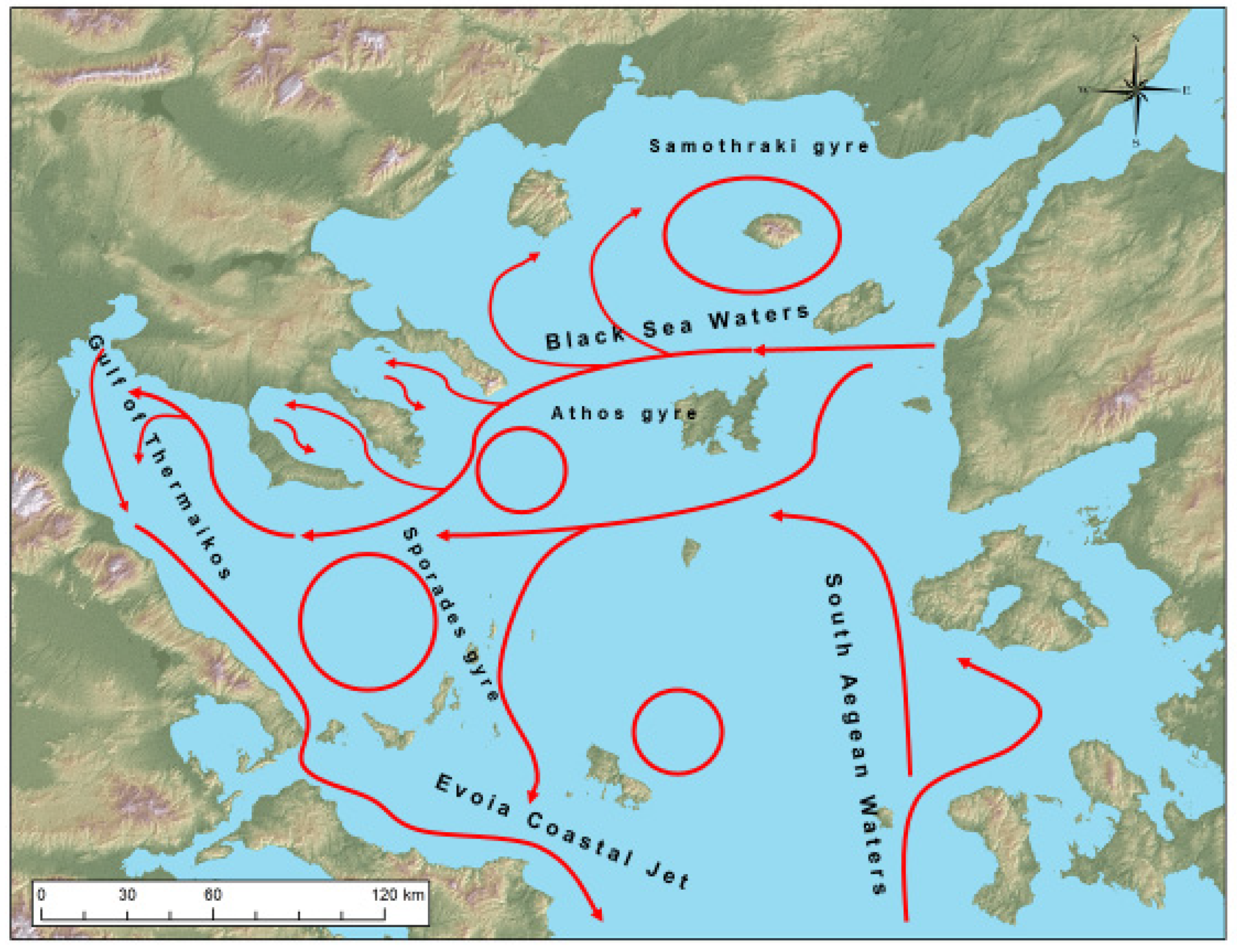
In order to illustrate the geospatial web service potentials, a well-defined case study area in Greece is used (
Figure 1). The study area is located in the North Aegean Sea. The North Aegean is characterized by lower salinity levels (29 psu) compared to the South Aegean (>38.5) [
23] and colder waters. The main contributing factor for the low salinity and temperature is the mixing from the outflow of the Dardanelles Strait, where waters from the Black Sea with an annual variation of salinity of 19–22 psu and a mean temperature of 16 °C penetrate the Aegean [
24]. Another significant influencing factor for the decreased salinity is the freshwater input from major rivers in the Thermaikos Gulf.
The low salinity and cold waters from the Black Sea influence the Northern Aegean Basin circulation, and they are the main reason they distinguish the Northern from Southern Aegean basin. The Black Sea waters, after entering the Aegean, they are divided into two main masses, the first flows to the North towards the Sea of Thrace and the second flows southern, towards the Sporades islands and then reaches the Southern Aegean through the Kafireas and Mykonos-Ikaria straits [
25]. Two major anti-cyclonic formations are present at Limnos and Samothraki islands and a smaller one western of Thasos Island [
26]. Another cyclonic formation can be observed at the Sporades archipelagos, which changes seasonally to an anti-cyclonic one. The flow from this formation continues to the South, along the Eastern Coastline of Evoia island, creating a strong and narrow coastal current.
2.2. Data
The dataset used in this study is derived from the Copernicus Sentinel-3 satellite data-stream. Thermal front detection is based on the Sentinel-3 SLSTR sensor which is equipped with 11 bands; S1–S6 are used for cloud detection and vegetation and ice monitoring at 500 m resolution, S7–S9 are used for Sea Surface Temperature (SST) and Land Surface Temperature (LST) estimations and fire monitoring at 1km resolution and lastly F1 and F2 for active monitoring also at 1km resolution. SST data already processed to Level-2 from the European Organization for the Exploitation of Meteorological Satellites (EUMETSAT) at a 1km resolution used for further analysis. The data are not interpolated but they provide cloud and pixel quality masks.
Sentinel-3 SLSTR imagery’s spatial and temporal properties where the most suitable choice for this application. The high 1km resolution of the SST data is well suited for the differentiation of small enough features, for both mesoscale and submesoscale features. Furthermore, with a swath of 740 km oblique view and 1400 km in nadir view, it covers the whole of the study area without the need of mosaicking. Finally, on the operational side of the service, the sensor has a temporal coverage over the Aegean of 1-2 days, enabling the servicing of daily products.
Level-2 SST data are acquired from the EUMETSATA Copernicus Online Data Access service. The data are stored by the Standard Archive Format for Europe (SAFE), containing the bands (NetCDF) and the manifest header file. A script is run daily searching for newly archived data based on spatial and temporal criteria. If there are data matching the query, their unique product ID is collected and then a URL request is generated for downloading each product, e.g.,
https://coda.eumetsat.int/odata/v1/Products(’ID’)/$value.
2.3. Methodology
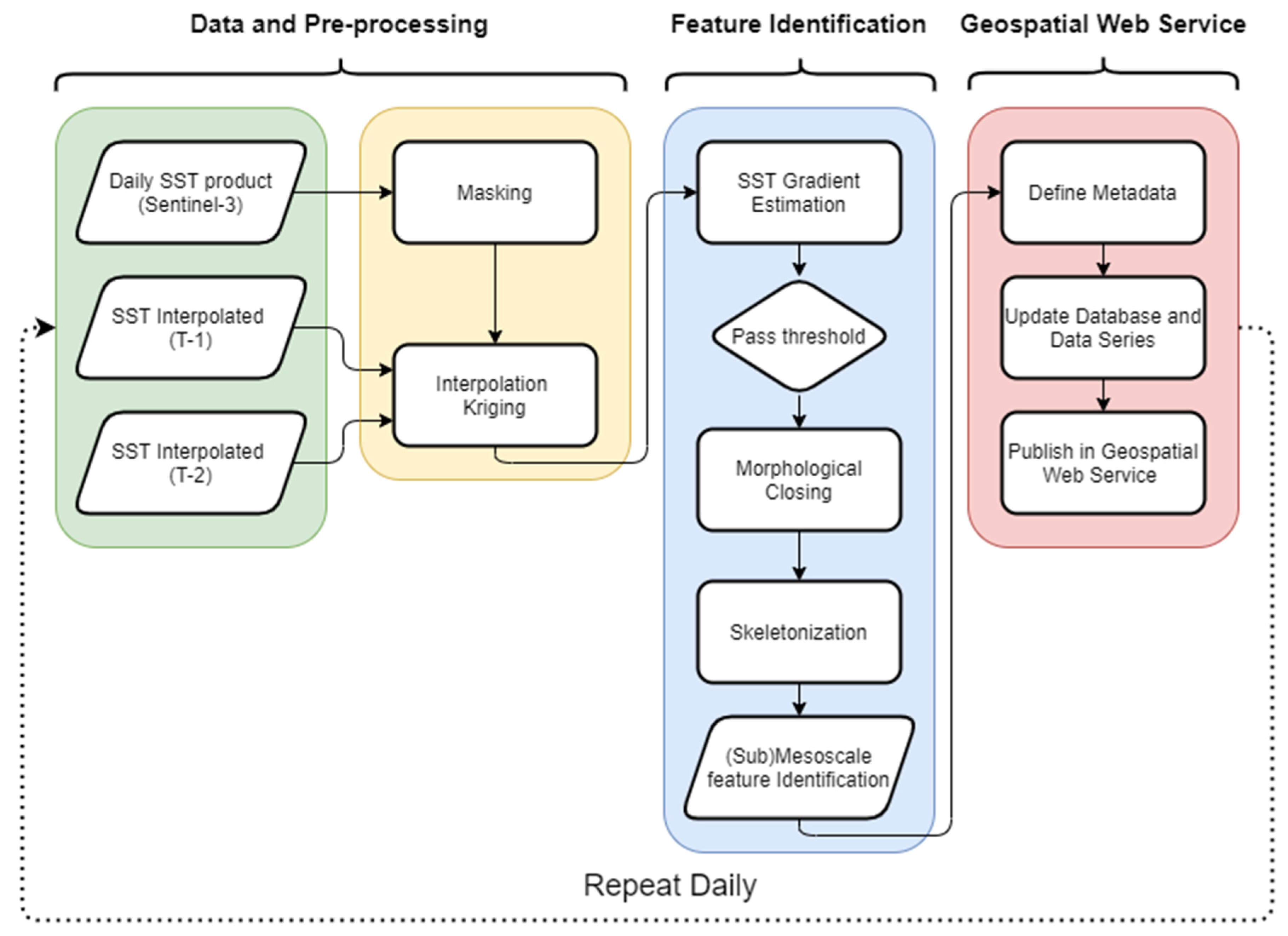
A fully operational service is presented to produce daily mesoscale and sub mesoscale oceanic feature localization maps. The service has three main sections: (a) obtaining the raw satellite data and pre-processing them in order to be used for the detection algorithm; (b) the detection process that produces the maps for the end users; and (c) the implementation of the geospatial web service, that publishes the end results according to the OGC standards (
Figure 2).
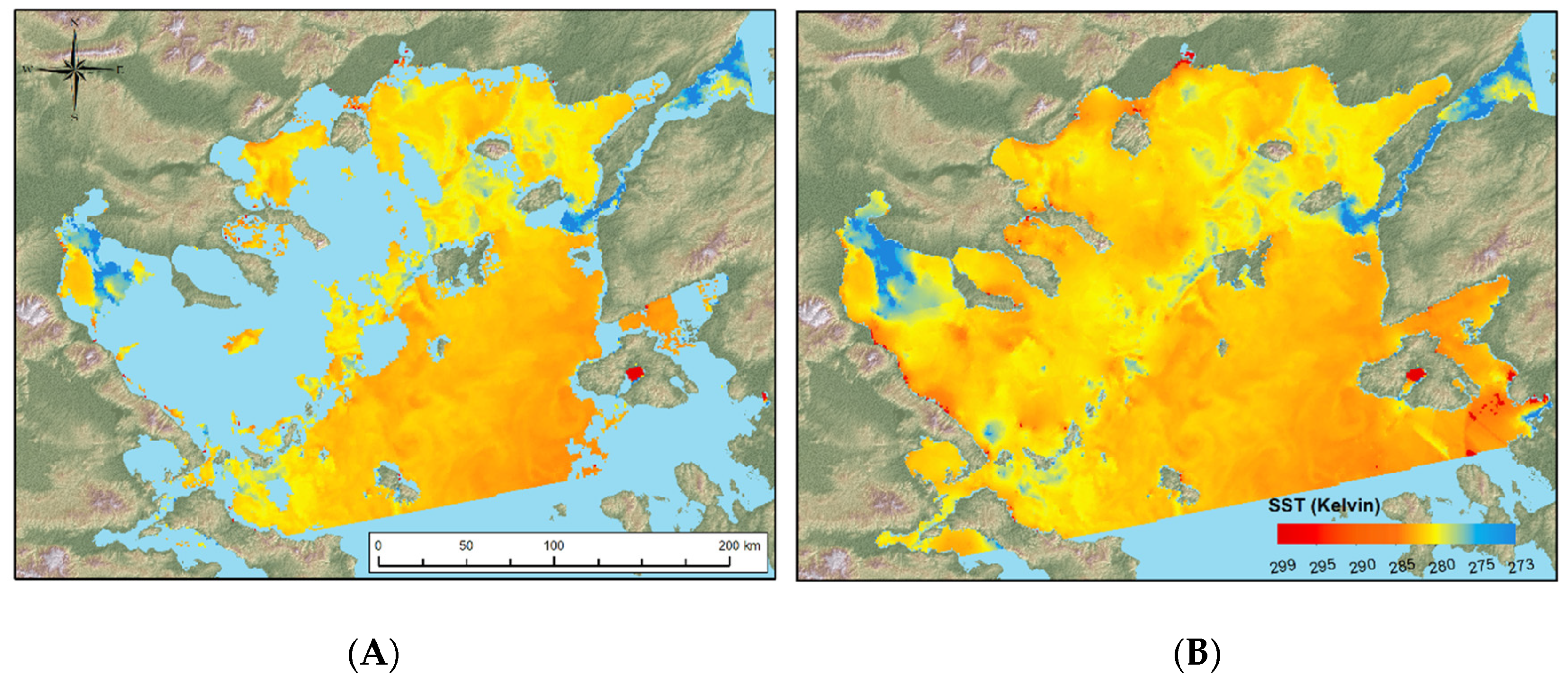
2.3.1. Preprocessing—Interpolation
In an effort to investigate the fluctuations of SST, a number of remotely sensed data were used over a number of timespans for the study area. Primary data include unwanted objects such as cloud coverage and land surface cells, which are not relevant to our research question. Thus, there is the need to remove (a) cloud coverage cells and (b) land surface cells as well as (c) extreme values near the coastal areas. The latter are considered to be data “noise” because of the anthropocentric activities nearby, the river outflows and the possibility of low bathymetry. A 5 km buffer zone around coastlines has been excluded. Cloud and land pixels are removed with a masking approach.
After this cell removal activity, there is a need to evaluate SST for the cell locations over sea. This is a typical spatial interpolation problem where some observations are used in the study area aiming to estimate values of a variable on locations with no information [
28]. In this paper, these observations are extracted from the same SST data that need to be interpolated and from values derived from data of the previous two days, represented as (T-1) and (T-2). All possible combinations of these datasets are tested for the interpolation modelling and are evaluated according to their accuracy.
For the estimation of values in locations with no information, the well-used Kriging group of spatial interpolation methods are introduced. Kriging is a broad family of interpolation methods with the advantage that it minimizes the estimation variance and error estimation, using a model of spatial covariance acquired by a semivariogram, so it has homoescedastic characteristics [
29]. This is a detailed understanding of the spatial variability which comes quite handy in estimating a variable in location with unknown values. The semivariogram is essentially the mean squared difference between pairs of values as a function of increasing separation distance (lagged distance). More details regarding semivariogram is given by Lamorey and Jacobson (1995) [
30]. Two variations of Kriging are tested: Ordinary Kriging and Co-Kriging. For both Kriging and Co-Kriging, a fundamental assumption is that the measurement data are normally distributed across the study area both in terms of statistical distribution and geographical distribution [
31].
The first method, Ordinary Kriging, implicitly evaluates the mean in a moving neighborhood. It is a weighted average estimation of values while weights are based on Best Linear Unbiased Estimator (BLUE). The second method, Co-Kriging, is used when estimating a single variable from several other variables. There should be a theoretical relationship between the variables of the model. Thus, the covariates must have a statistically strong relationship as well. This approach asks for the spatial covariance model of each extra variable as well as the cross-covariance model of the variables. A couple of Co-Kriging estimations were created with different variables. The two attempts included the following sets of variables: T ~ (T-1) and T ~ (T-1) + (T-2).
The evaluation of the performance of Kriging Interpolation was achieved with a classical Data Mining “Leave Out” approach. This is the split of the initial dataset into two group of cases. The first group includes 500 randomly sampled observations which have been excluded from Kriging estimation. This sample serves as the “evaluation group” and it is used only during accuracy assessment of the results. Rest of the cases (n = [8500, 9000]) are used for Kriging estimation.
After estimating values for all locations of the study area, the n = 500 evaluation sample is used for calculating the deviation between estimated values (result of Kriging) against empirical values (evaluation sample data). A group of accuracy metrics are used to compare the two values for the n = 500 observations. These two measures are based on the squared errors, i.e., mean absolute error in Equation (1) as well as the absolute error i.e., root mean squared error in Equation (2).
where
ei is the difference between the estimated SST value and the corresponding evaluation data at grid location
i. The two measures are scale-dependent, which do not affect the outcome of the measures as sample size (n = 500) is constant across all estimations over time spans.
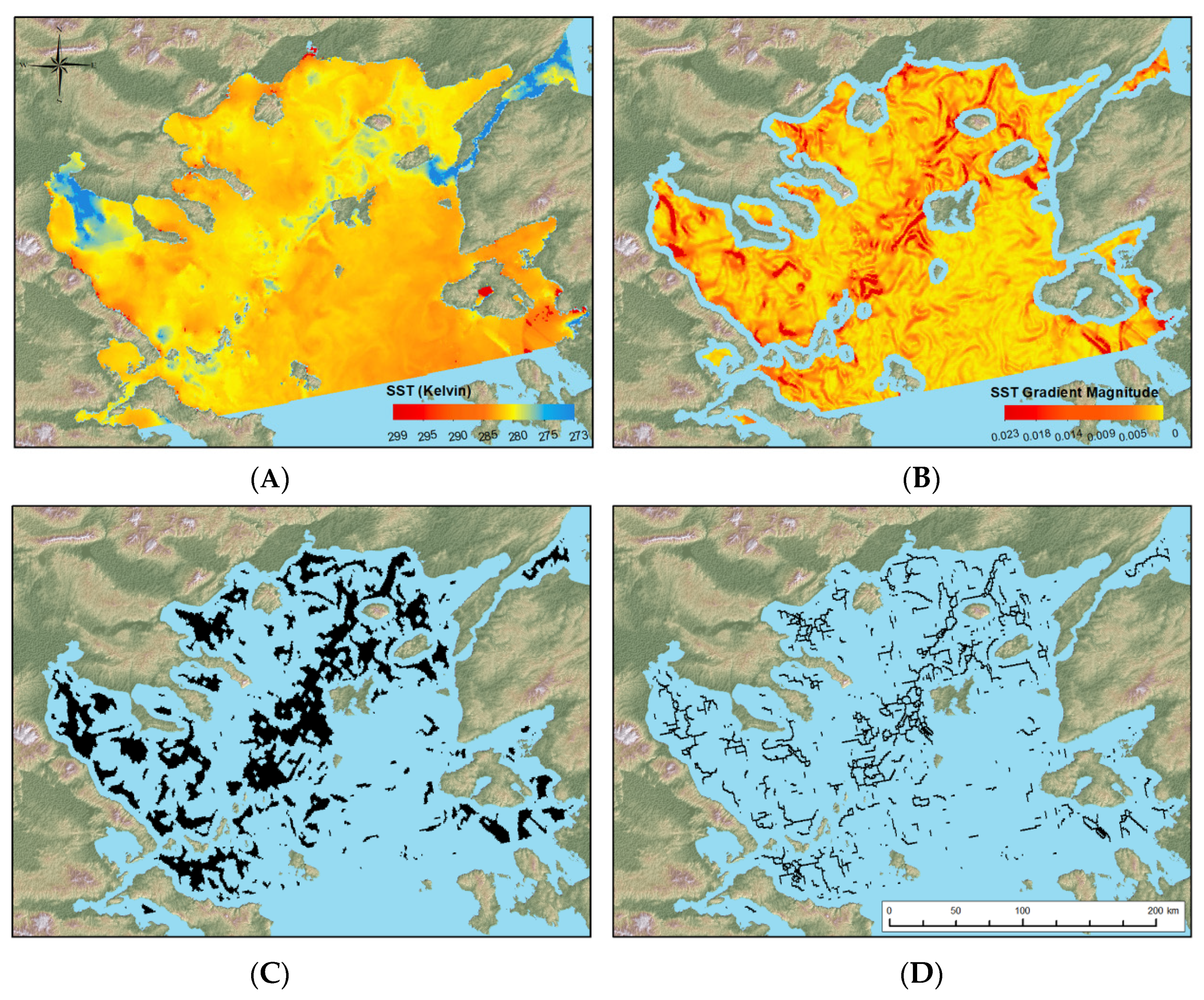
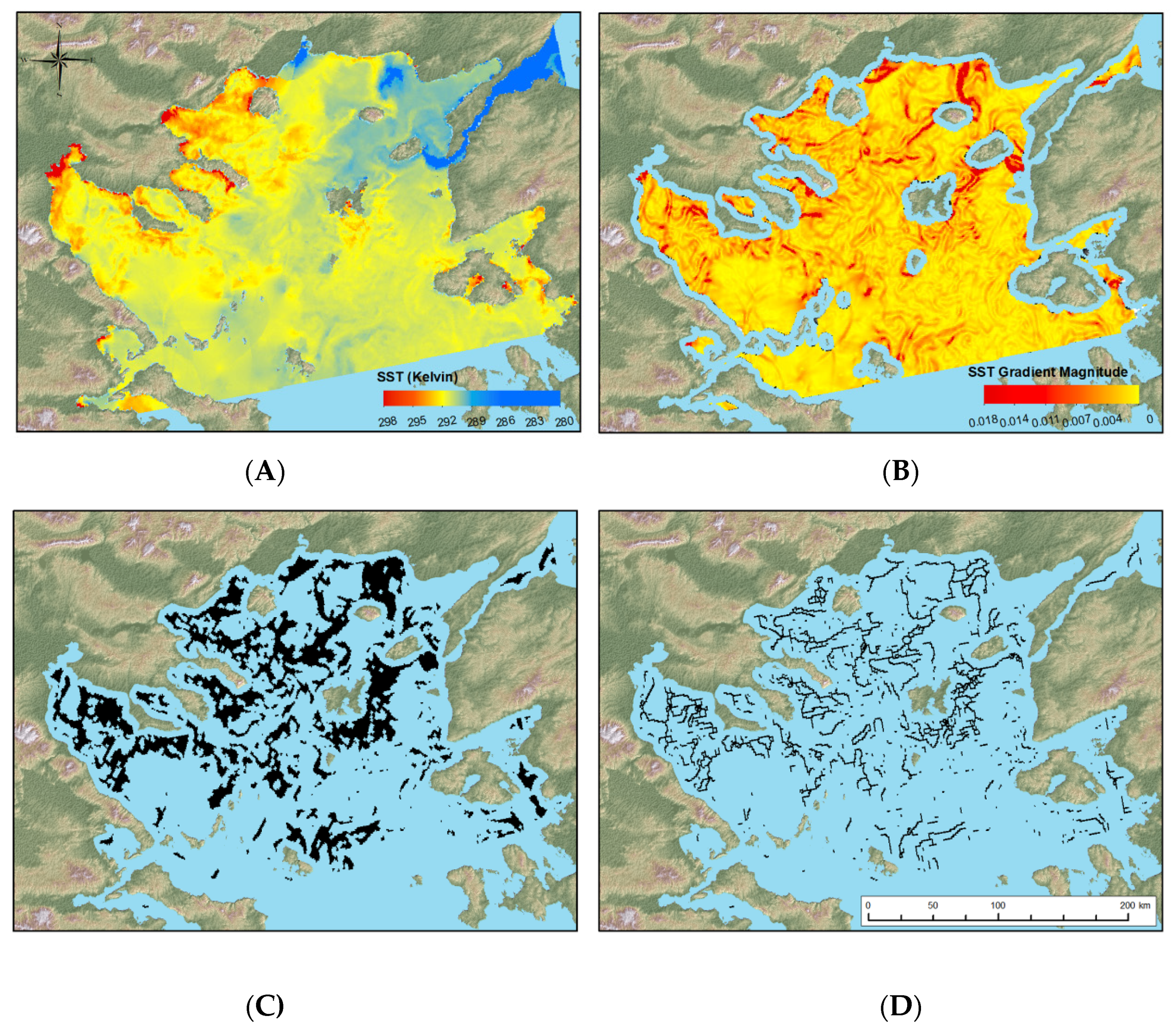
2.3.2. Oceanic Front Detection
The circulation formation detection method stands on the premise that different water bodies have different physical attributes. It is based on the thermal front gradient detection method [
13], which is an edge detection technique for image analysis. A filter is used to identify areas that there is a sudden change of temperature in neighboring pixels. These areas are usually the meet points of different currents that create an eddy, the fringes of a gyre or a cyclonic formation. This category of thermal front detection methods is prone to noise due to inherited low gradient magnitude that characterizes the oceanic flows, but they are very lightweight procedures, making them excellent for operational and automated services.
For the edge detection, the Sobel operator was used [
32]. It is a moving window-based operation that compares each pixel with their immediate neighborhood. Peak values are found at pixels where a sudden change in SST occurs. The operator performs the gradient estimation separately for the x and y axis of the image, by calculating the directional gradient of the SST (Equations (3) and (4), respectively). Those directional gradients are then used to calculate the overall magnitude on the image (Equation (5)). The points where the gradient reaches its peak, are marked as potential edges according to the following equations.
where
Imn, the SST image of day n,
Gxn and
Gxy the SST gradients for the x and y axis, respectively, and
Gn the overall gradient magnitude.
Not all the regions are oceanic fronts though. Pixels can produce some level of gradient magnitude for various reasons not always associated to oceanographic phenomena, such as: sensor noise, shallow areas near the coastline, river outflows and the edges of clouded areas. For that reason, distinction must be made between the possible oceanic fronts and the false positives pixels. Generally, gradient values produced by noise in the image are on the lower range, and those related to coastal processes and clouds at the top extremes. In order to extract only the useful information concerning the oceanic features, a double threshold is performed according to the interquartile ranges of the image histogram. Ranges between the first and fourth quantile are considered pixels with weak gradient magnitude values and those above the fifth pixels related to noise or extremes. These ranges are automatically redefined for each new image and are adapted accordingly.
The weak gradient magnitude that characterizes oceanic processes also has a different effect on thermal front detection, that it occasionally produces discontinuities. Specifically, pixels at the center of a front may have a weak gradient signature and, as thus, they fail to pass the threshold value and split the front into multiple parts. To overcome that effect, a morphological closing technique is applied to the thinned edges. After the threshold is performed, the resulting image is transformed to a binary one, whether each pixel has a strong magnitude signature or not. Next, the closing takes effect and it connects pixels that are in proximity to each other in order to make more coherent objects.
Even though a general positioning of the oceanic features has been established, the localization is not yet accurate enough. At the meeting point of two currents there is usually a mixing zone and if so three water masses are created with different characteristics. The first and second are the two meeting currents with their own separate physical attributes. The third is the mixing zone around the thermal front with characteristics based on the two mixing flows. As such, edges from thermal fronts are not sufficiently strong and the gradient magnitude produces high values around the edge. To compensate for that effect, a skeletonizing technique is applied to reduce the edges to a single pixel line positioned at the center of the edge. The thinning works by comparing each pixel with its neighbors and decides whether to reduce it to a 0 based on a set of rules [
33].
It should be stated that the lack of in-situ data renders the evaluation and the accuracy assessment of the results difficult. To combat this limitation, a visual comparison is performed between the produced oceanic features and the known general circulation conditions of the North Aegean sea.
2.4. Service Structure
Although research institutions and universities produce a significant amount of quality geospatial data during research activities or educational processes, they usually fail in the proper maintenance and distribution of the provided information [
34]. Consequently, valuable scientific datasets are scattered among numerous departmental and laboratory computers, without any provision of exploitation by the wide research community. To overcome this issue and to keep up with the movement of Open Science and the pertinent National Plan of Greece [
35], a Spatial Data Infrastructure (SDI) was developed within the Marine Remote Sensing Group (MRSG), University of the Aegean. The promotion of access to geographic information aims to encourage its publication as open data, i.e., freely available to everyone to use and republish as they wish, without restrictions due to copyright, patents, or other control mechanisms [
36].
SDIs facilitate the discovery, access, exchange and sharing of geographic information and services among stakeholders from different levels in the spatial data community [
37] and they are an essential tool for institutional data dissemination [
38]. They also support decision-making processes and planning activities concerning environmental management and nature conservation [
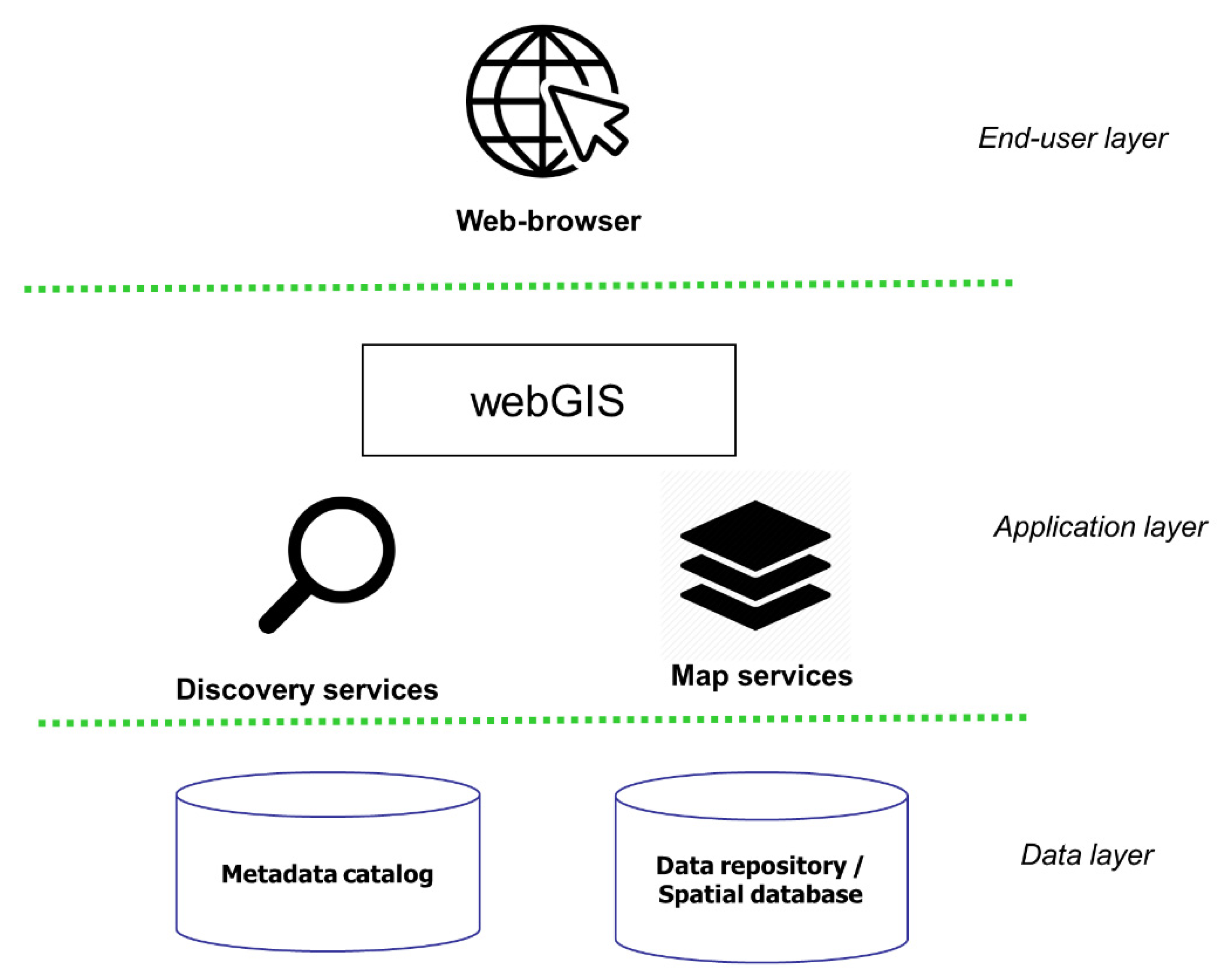
39]. An SDI is considered as an amalgam of data, technologies, standards, policies and people.
Figure 3 depicts the general architecture of an SDI. In the following paragraphs, the components of the MRSG SDI and its operation to support data organization and diffusion of the mesoscale oceanographic feature identification task are presented.
Three datasets will be published to the service, the finalized skeletonized oceanic feature data, and both the raw and gradient magnitude datasets for reference. The oceanic features are in a vector file format in order to be able to store geographic information for each specific object. These data are stored in a PostgreSQL-PostGIS based database, with geographic object queries support, allowing for spatial and temporal interconnectivity between data from different dates.
All datasets related to the procedures of this paper are documented according to the ISO 19115 Metadata standard for geographic information [
40]. In this way, the output datasets are uniformly described in a precise and complete manner and they are discoverable through open interoperability protocols (like OGC CS/W service,
www.ogc.org/standards/cat). The GeoNetwork opensource platform (geonetwork-opensource.org) constitutes the metadata catalog of the SDI, as it provides a number of powerful capabilities, such as metadata editing, validating and search functions, monitoring and reporting tools, API and customization facilities and Free and Open Source Software principles support.
The creation of new metadata records is supported by an in-house developed tool that produces XML files to be imported into the GeoNetwork platform. The Purpose metadata attribute is used to discriminate the type of the dataset (i.e., raw SST data, gradient estimations, output skeletonized vector files). Other attributes—such as Title, Abstract, Keywords, Topic category, Lineage, Resource constraints, Data quality information, Metadata details and Contact information—are automatically filled in, according to the Purpose and Date attributes. The Distribution information metadata attributes are used to provide the appropriate links to the data repository and the map server (described subsequently).
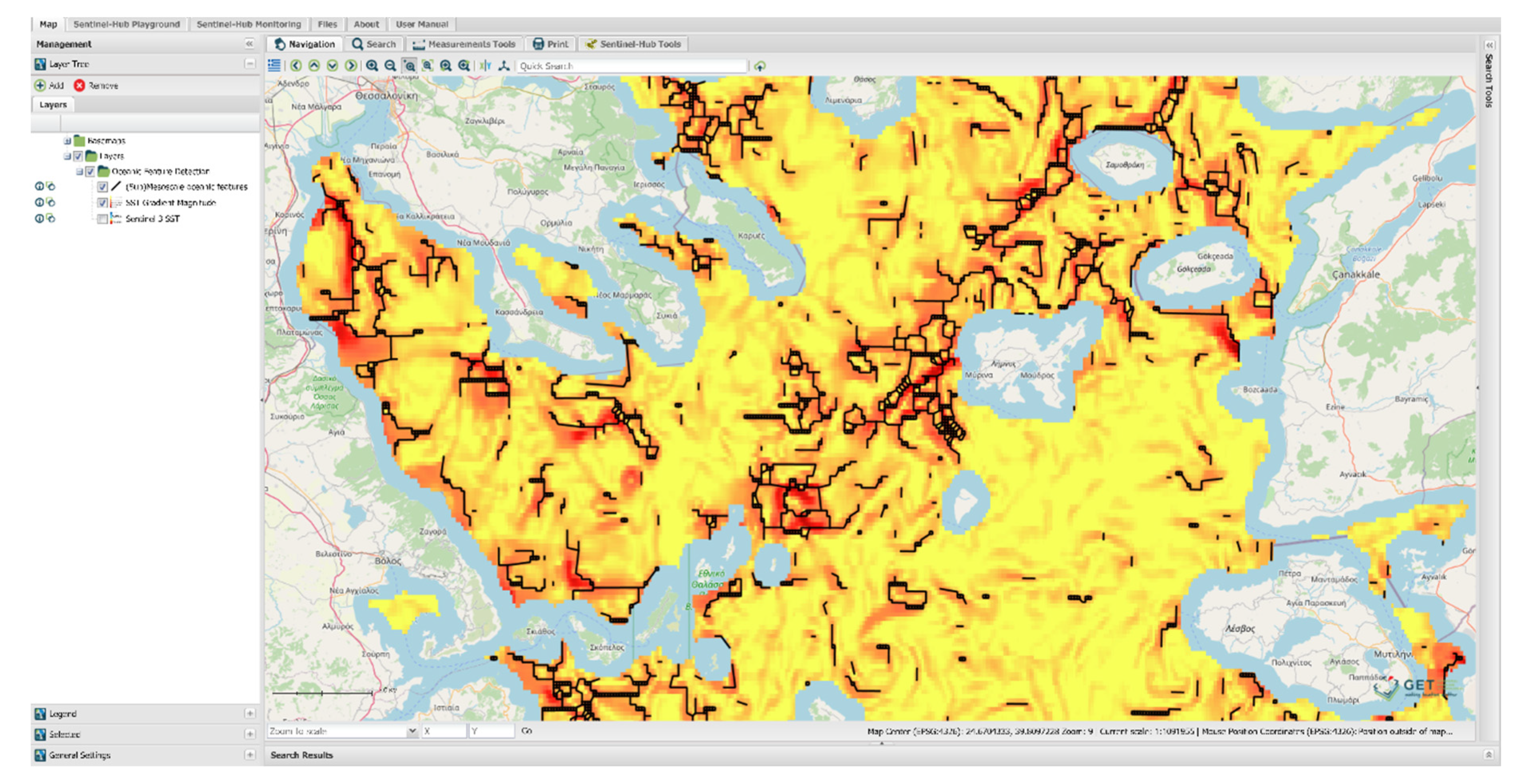
For the visualization, cartographic navigation and downloading of the output products, OGC services are utilized (like WMS, WCS, WFS). Specifically, by exploiting the capabilities of the GeoServer open source map server, all datasets are automatically transformed to interactive map layers that end-users may access, display, query and download using a webGIS platform. The Metadata links and Data links attributes of the GeoServer layer editor are used to record the appropriate links to the metadata catalog and the data repository, respectively. End-users of the SDI may have full access to all datasets by activating different layers into a webGIS platform granted by the GET (Geospatial Enabling Technologies,
www.getmap.eu) company.
The layers are based on the geographic web services already developed and published into the map server. The webGIS mainly consists of an interactive map and provides user-friendly cartographic operations for visualizing and manipulating thematic maps (like map navigation, overlay, base-map selection, etc.), as well as querying, measuring, printing and downloading operations. The adoption of metadata standards and open interoperability protocols for geospatial information has contributed to the increase in recognizability, accessibility and reusability of the products resulting from our work.
4. Conclusions
In this paper, a new geospatial web service implementation is proposed, for providing spatial information on mesososcale and submesoscale processes in the North Aegean Sea. Daily oceanic feature identification maps are produced reliably with a gradient edge detection technique. These processes are encapsulated in a web-based SDI, and the final results are serviced to the end-users ready for use, either for visualization and quick decision purposes or for direct downloading.
The widespread availability of Sentinel-3 satellite data has enabled the extraction of more robust, fine and accurate information. Both temporal and spatial resolutions of the SLSTR sensor have proven that methodologies can be applied for smaller object identification and with smaller periodic cycles. These data are also ready to use and built for convenience, providing already processed data at Level-2, equipped with both cloud and land masks and pixel quality flags.
The proposed methodology combines reliability with simplicity. It is based in a process which is well studied from previous works, modernized, and optimized for current technologies and data. Capable of identifying features at scales bellow 5km in diameter, it has proven that can be applied to both small- and large-scale oceanographic applications. It is not without its flaws, however, as it is sensitive to high gradient magnitude signals it fails to capture features at more homogenous waters. Nonetheless, by not being a trained model but rather a series of image manipulation techniques, it offers great repeatability and correction of such defects should be simpler. Furthermore, as a non-data dependent methodology, it enables immediate application in other marine regions.
The proposed oceanic feature identification processing chain has produced promising results for operational services. Most of the important and impactful mesoscale and submesoscale circulation formations of the North Aegean have been successfully mapped. These data can be readily available through the webGIS interface for visualization and processing or they can be downloaded through open source means for use in various research fields. This is a powerful way to organize and distribute oceanographic data for daily use.
Moving forward, this service is planned to be updated and enriched with additional products as well as expanded for full coverage of the Greek Seas. The first major step towards the improvement of the (sub)mesoscale identification products is the inclusion of Sentinel-3’s OLCI data, as chlorophyll fronts play a vital role in the fish population distribution. Data from the OLCI sensor can provide chlorophyll-a concentration estimations at a spatial resolution of 300 m, enabling the possible detection of even smaller scale processes. Furthermore, the SLSTR’s swath completely overlaps OLCI’s and both datasets can be used in conjunction, detecting both thermal and ocean color fronts, integrated in one product. These products, along with the fine-tuned existing ones, will be used to map the oceanographic processes in the North and South Aegean Sea daily, as well as in the Ionian Sea. Secondly, a statistical quality assessment of the results must also be performed with the use of in-situ measurements, so that any shortcomings can be pin pointed and corrected accordingly. Finally, as one of the goals of the geospatial web service is to work as a decision-making tool for maritime authorities and the fishing industry, a set of marine navigation tools will be incorporated, such as route planning and weather and wind forecast display.


