1. Introduction
The remarkable propulsive and manoeuvring mechanisms of aquatic swimmers, that have fascinated researchers since the 1970s, inspire the design of modern autonomous underwater vehicles (AUV) as well as autonomous underwater gliders (AUG) for marine environmental data acquisition, see, e.g., [
1], biomimetic swimming robots and novel propulsion devices with enhanced efficiency, see, e.g., [
2]. Selection of the swimming mode to serve as inspiration for the artificial devices closely depends on hydromechanical aspects of the application itself. The thunniform swimming mode for example, where the caudal fin of the fish performs a combination of pitching and heaving motions, identifies as the most efficient and therefore suitable for nature-inspired propulsion systems operating at high cruising speeds, see, e.g., [
3,
4]. Devices based on flapping foils have also been studied as auxiliary thrusters augmenting the overall ship propulsion in waves, see, e.g., the works [
5,
6,
7,
8,
9] and project BIO-PROPSHIP [
10]. Moreover, oscillating foils are studied for the development of hydrokinetic energy devices, see, e.g., [
11,
12,
13] or hybrid devices with enhanced performance exploiting combined wave and tidal energy resources, see [
14].
Living organisms through natural selection have been able to further enhance their locomotion capabilities through passive or active deformations of fins. In this direction, computational and experimental work on the principal mechanisms for thrust production in flexible oscillating bodies can be found in the review [
15] with emphasis on aquatic locomotion as well as the works [
16,
17] regarding aerodynamics and aeroelasticity. Further investigation on the parameters that result in performance enhancement of flexible systems remains essential for the development of successful engineering applications in the future.
Over the years many researchers have presented mathematical models and numerical schemes to tackle this complex fluid–structure interaction (FSI) problem. One approach is to assume that the deformations are known a priori, see, e.g., [
18]. The coupled problem can also be treated with strongly coupled methods; i.e., a fluid flow solver used in conjunction with a structural solver, employing iterative processes to solve the coupled problem of passive deformations, see, e.g., [
19,
20].
Notable is the approach by [
21,
22] to investigate thrust production in flexible wings with a potential-based model. Later, [
23] presented a potential-based 2D flexible body vortex sheet model to estimate propulsive forces and optimal efficiency, which was further validated experimentally in [
24]. Fully coupled FSI simulations for flapping wings with chord-wise and span-wise flexibility were carried out in the work of [
25], with extensions in [
26] allowing even the study of skeleton-strengthened fins. By employing the vortex-based method for the fluid flow problem along with a finite difference method for the structural response problem as presented in [
27] it is shown that chord-wise flexibility enhances up to 10% the propulsive performance of a flapping-foil thruster for AUV’s.
The effects of flexibility in propulsive performance enhancement are also illustrated in experimental works, see, e.g., [
28,
29,
30]. The effects of flexibility on the time-averaged thrust can be beneficial for plunging foils even when the flexible region is confined to a small section near the trailing edge, see, e.g., [
31], compared to rigid foil cases. Moreover, proper selection of chord-wise flexibility characteristics in 2D foils in flapping regimes leads to up to 36% increase in efficiency compared to rigid ones, see, e.g., [
32]. During experiments on elastic flat plates it has been observed that the more flexible plates showed enhanced propulsion characteristics, see, e.g., [
33]. Other works [
34,
35] both theoretical and experimental, investigated the structural response of flexible flat plates under heaving motions. The experiments revealed that the thrust displayed peaks in motion frequency values coinciding with the resonance frequencies of the system comprised of the foil and the surrounding fluid. Following a different approach, see, e.g., [
36], the propulsive performance of a flapping system that allows different inclinations of the robotic fin tip has been studied in terms of propulsive efficiency. Despite the increased efforts and contributions in this field, investigation on the parameters that result in performance enhancement of flexible systems remains essential for the development of successful engineering applications in the future.
Especially for fluid flow problems at high Reynolds numbers, moderate angles of attack and Strouhal number, which is the operating regime for marine thrusters, potential-based methods have proven to be suitable for the study of elasticity effects on thrust production. In that sense, lower-fidelity and cost-effective inviscid fluid flow simulations are a useful tool in the preliminary design phase of biomimetic thrusters, where emphasis is given on parametric studies, whereas high-fidelity CFD simulations, see, e.g., [
37], are more computationally intensive and resource demanding compared to potential-based solvers. A direct comparison between the two approaches can be found in [
38].
The scope of the present work is to propose a non-linear fully coupled BEM–FEM scheme for the solution of the FSI problem of chord-wise flexible flapping foils operating as marine thrusters, including thickness and flexural rigidity profile variation. The major contribution of this work is that the developed method and software could serve, after enhancement and further validation, as a useful cost-effective tool for the preliminary design and optimum control of flexible biomimetic thrusters. Although the proposed cost-effective method is less accurate than high-fidelity CFD methods at specific regions of the operational parameters (large angles of attack and Strouhal number), it is suitable for the investigation of the effects of flexibility on the propulsive performance of such systems, the accurate prediction of hydrodynamic loads as well as the structural response of the foil.
In the present formulation, the flexible foil performs prescribed oscillatory motions and is free to deform under inertial and reactive forces caused by its motion and hydrodynamic pressure. The hydro-elastic analysis is based on a non-linear time domain boundary element method (BEM) for the unsteady lifting flow problem and a high-order finite element method (FEM) for the prediction of the deformed body geometry using the Kirchhoff–Love thin plate theory for cylindrical bending under plane strain conditions. The foil is considered clamped at a position along chord length, while its trailing edge (TE) and leading edge (LE) act as free ends. The structural and hydrodynamic aspects of the problem are coupled in an implicit manner, encapsulating forms of non-linearity.
The structure of the paper is as follows: In
Section 2, we describe the physical problem of a flexible flapping-foil thruster.
Section 3 presents the mathematical formulation of the hydromechanical problem and
Section 4 the numerical methods as well as the proposed BEM–FEM coupling schemes. In
Section 5 we present numerical results consisting of a convergence study and comparisons of the method with experimental data. The effects of elasticity over a range of design parameters, including Strouhal number, heaving and pitching amplitudes are presented and discussed in a series of parametric numerical studies, illustrating that chord-wise flexibility and flexural rigidity profile variations can significantly improve the propulsive efficiency of the biomimetic thruster. Conclusions and a short discussion are presented in
Section 6.
2. Problem Description
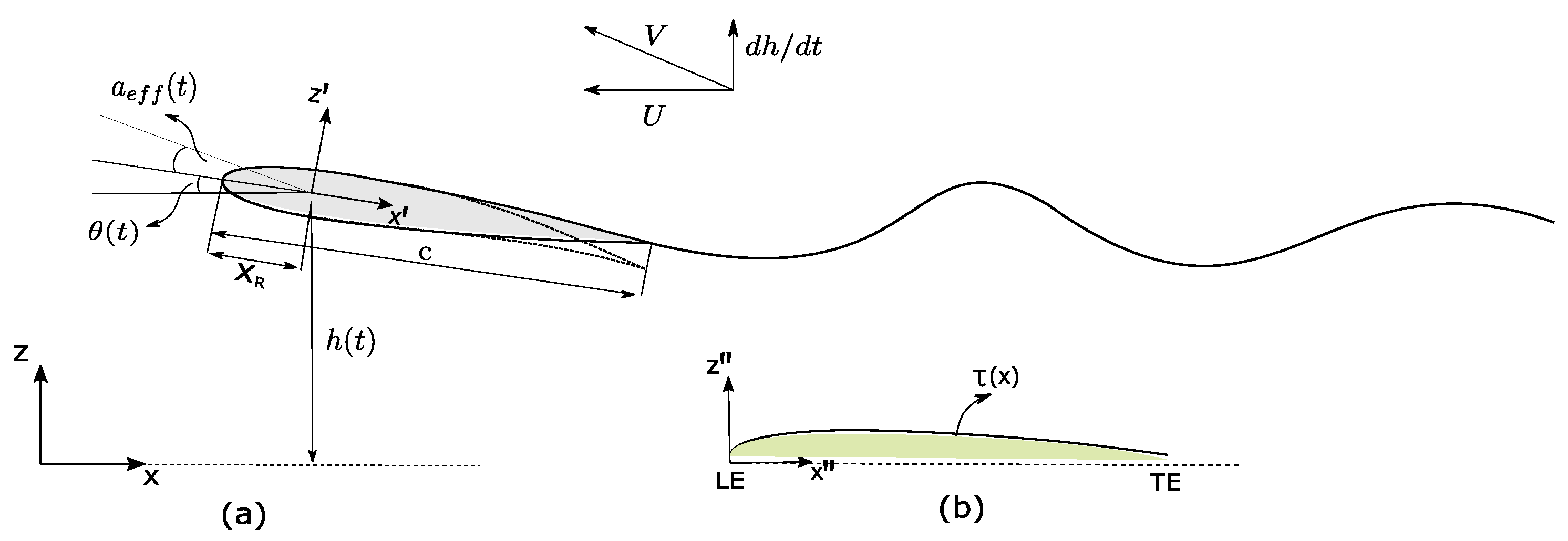
In the present work we consider the unsteady motion of a large-aspect-ratio rectangular foil with chord length
and thickness profile
, see
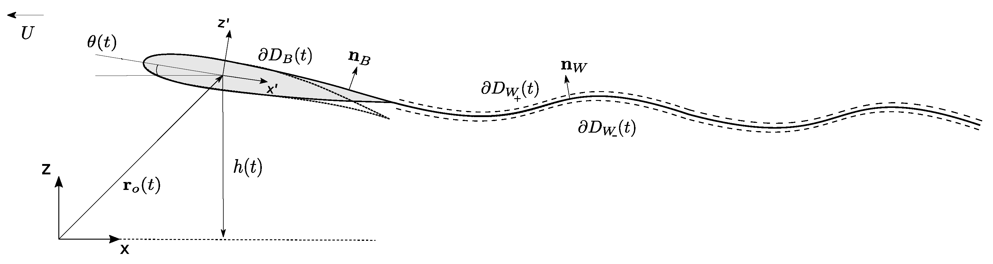
Figure 1. In general, a foil made of flexible material bends and twists in all directions. However, for large-aspect-ratio foils under the assumption of cylindrical bending, spanwise deformations are neglected. In this work, our aim is to predict the inertia and fluid-driven chord-wise deformations of a foil that undergoes large general motions. The following Cartesian coordinate systems are introduced in this work:
the space-fixed frame , with respect to which the foil moves in the negative direction of with constant cruising speed
the body-fixed (non-inertial) positioned at the foil’s center of rotation with in the direction of the un-deformed chord line
the body-fixed (non-inertial) position at the leading edge (LE). This frame is exclusively used for the structural response problem.
Additionally, the foil is subjected to a combination of harmonic heaving
and pitching
motions,
where
denotes the motion amplitudes,
the phase difference and
the oscillation frequency. In that sense, the effective angle of attack
is
For the hydrodynamic performance of flexible oscillating foils with large aspect ratio, the following modelling parameters identify as primary: (a) the non-dimensional heaving amplitude
; (b) the feathering parameter (ratio of pitching angle
compared to the maximum angle of attack induced by the heave motion
); (c) the phase angle between heave and pitch
; (d) the relative position of the pitching axis
(center or rotation) and (e) Strouhal number as a measure of unsteadiness
, where
is the flapping frequency,
is the nominal trailing edge amplitude, see, e.g., [
15]. In this study, the characteristic flexural rigidity
is also introduced, with
denoting the material density and
the acceleration of gravity.
5. Results
Regarding the BEM solver, as presented in
Section 4.2 for the hydrodynamic analysis of rigid flapping foils, extensive validation against experimental data as well as calculations concerning the solver’s numerical performance over a range of motion parameters can be found in [
49] and [
37]. An indicative comparison of the 2D-BEM and experimental data in the case of a rigid flapping foil is shown below in below in
Section 5.2, used as a reference for illustration of the effect of elastic deformation.
As concerns the accuracy of the present FEM solver, as a first example results concerning the free vibration analysis of tapered cantilever beams with taper ratio
are considered. The thickness distribution along the beam is linear. The relative error for the first five eigenfrequencies, between the present FEM for a mesh of
and the analytical solution from [
50], is listed in
Table 1 for two values of the taper ratio. The present method results are in excellent agreement with reference values and are further enhanced with refined discretization.
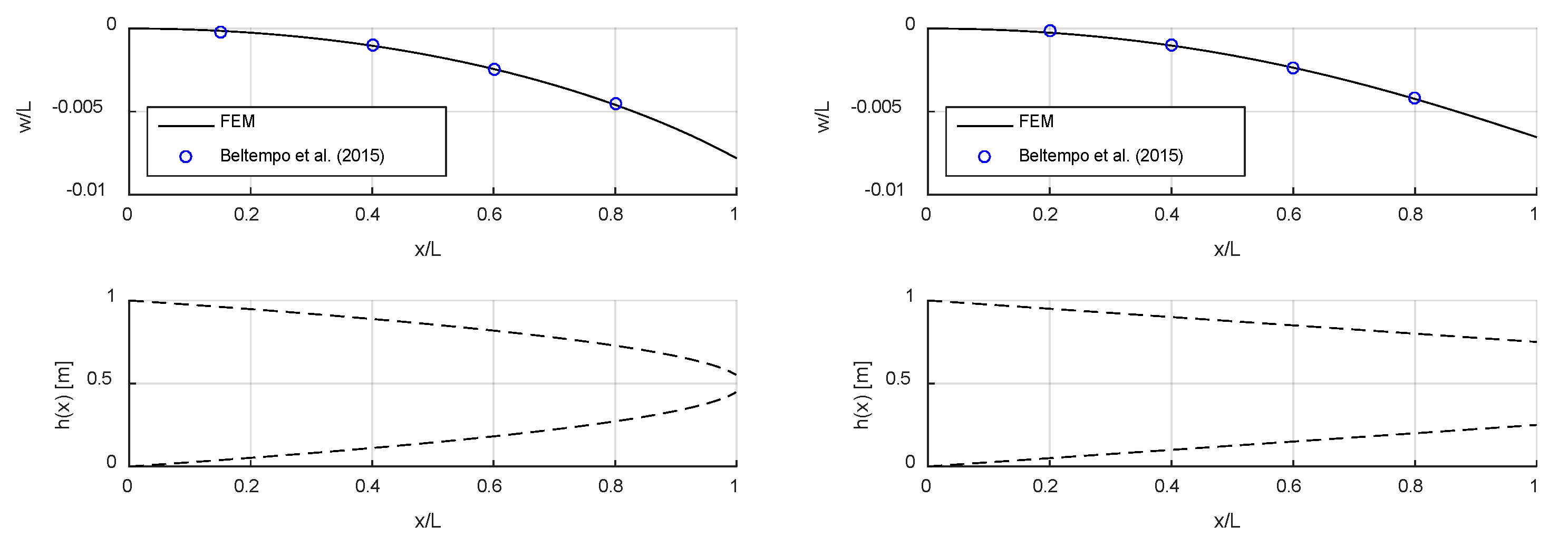
Another example concerns the static behavior of cantilever beams of length
of variable thickness under tip load forcing
; see [
51]. In
Figure 4, we present a comparison between the FEM and data obtained from [
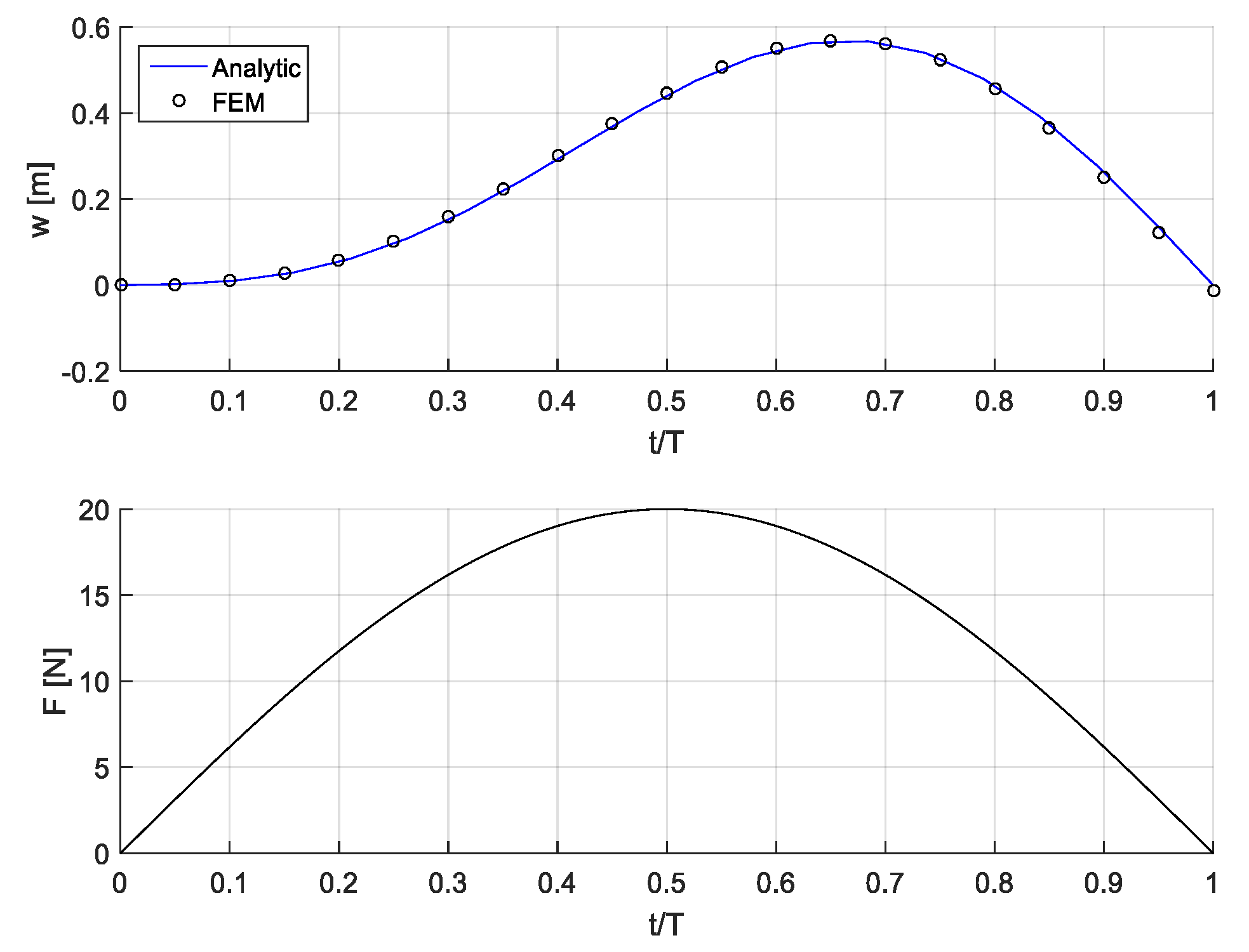
51] regarding the transverse displacement. Finally, the FEM solver is validated against a dynamic test case of a cantilever beam of a constant thickness profile, under transverse dynamic tip loading
The beam’s response in terms of tip transverse displacement profile is compared in
Figure 5 against the analytic solution presented in [
52].
5.1. Convergence Characteristics of the Numerical Scheme
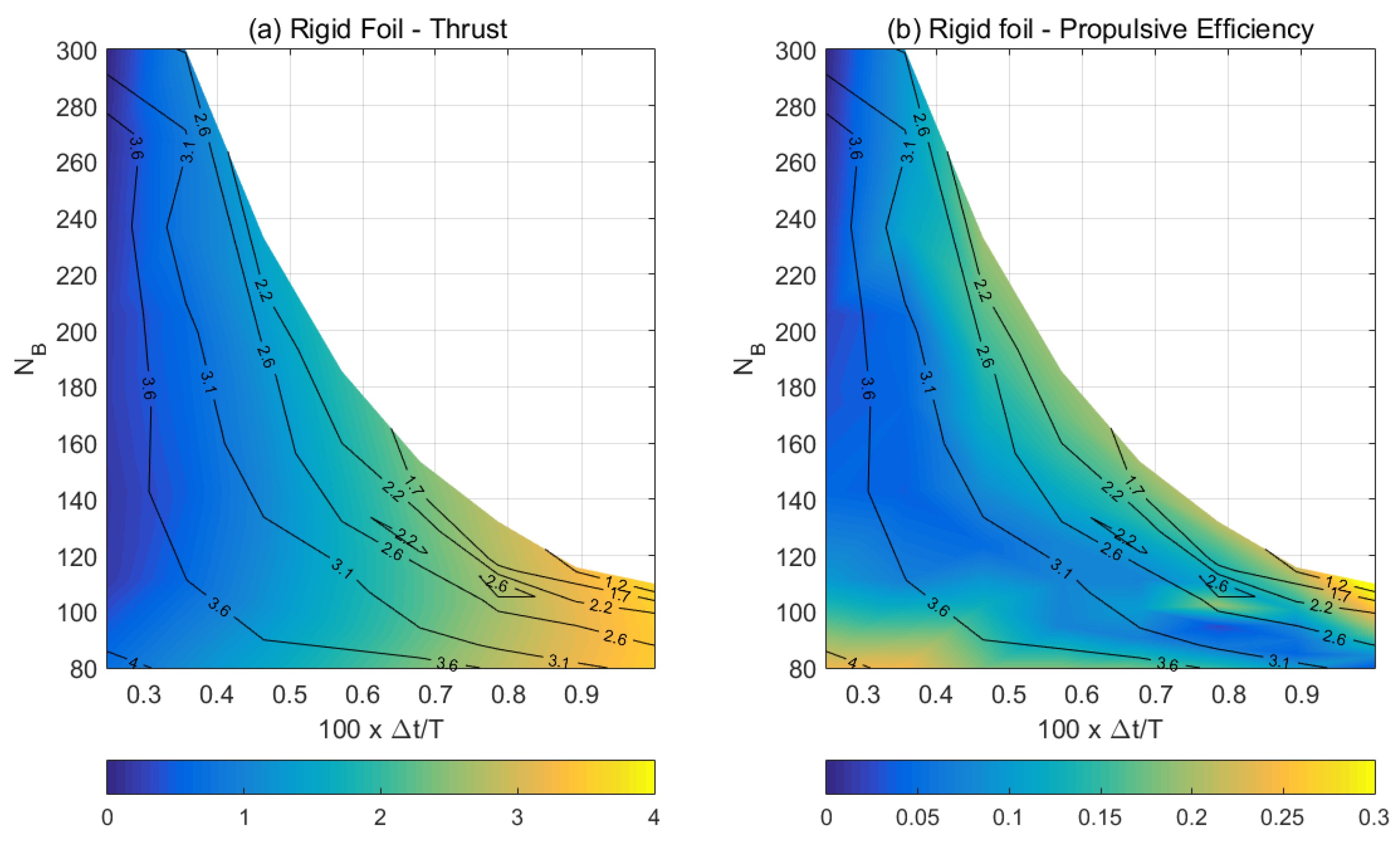
In this section, results concerning the convergence characteristics of the proposed numerical schemes are presented. To begin with the hydrodynamic problem, we present in
Figure 6 and
Figure 7 the relative error concerning the calculated thrust coefficient and the efficiency of a rigid flapping foil against the time discretization parameter
and the number of elements
subdividing the foil contour. The former represents the ratio of the time stepping over the motion’s period and the latter the characteristic panel length on the hydrofoil, whereas the contours correspond to constant values of the ratio
. The results were obtained using both solver options, as presented in
Section 4.2.2, including free wake modelling. Both numerical schemes converge for rigid flapping-foil simulations, i.e., the relative error is close to zero for the finest space and time discretization. In
Figure 6, we can observe that a coarse discretization in time corresponds to greater values of relative error (up to 4%). For the propulsive efficiency, the relative error is significantly lower for discretization domain (up to 0.3%). It is important to note that the Adams–Bashford method is not as stable, since simulations that correspond to a coarse discretization in time and a finer mesh in space lead to numerical instabilities, which explains the non-symmetric mesh-grid. Particularly, for
,
, the error is of the order of 0.5%, and thus the latter values are selected for the simulations.
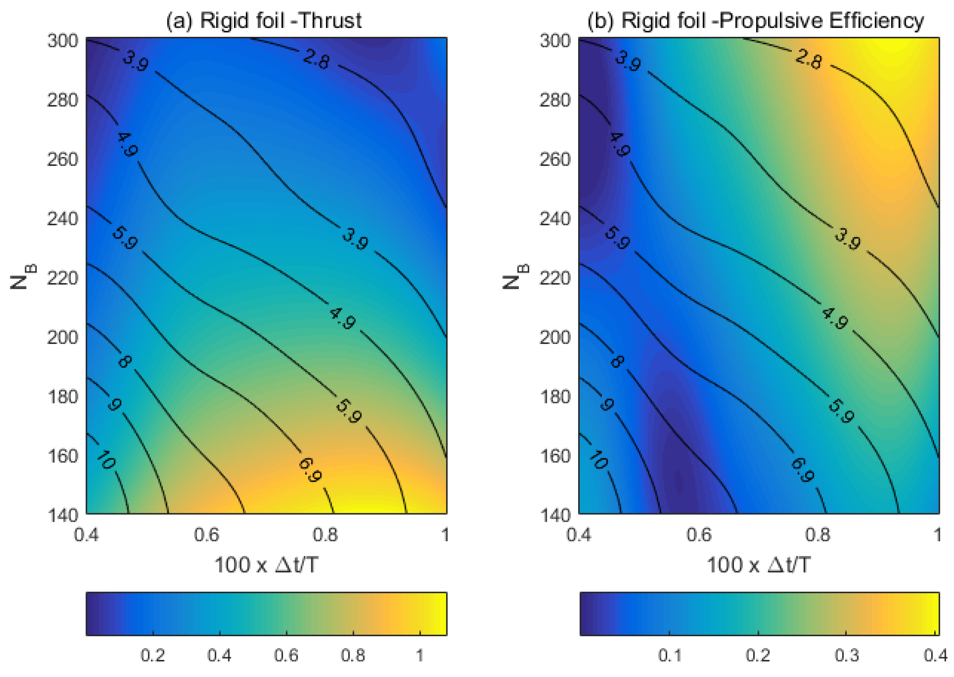
On the other hand, the BEM based on the Newton–Raphson iterative scheme shows a difference behaviour. In
Figure 7, the relative error has its maximum value of 1% and coincides with the region of coarse mesh both in space and time. This behaviour is a significant advantage that this numerical scheme shows quantitively along with the fact that it is more stable. Similarly, for
, the error is of the order of 0.25%, and thus the latter values are selected for simulations.
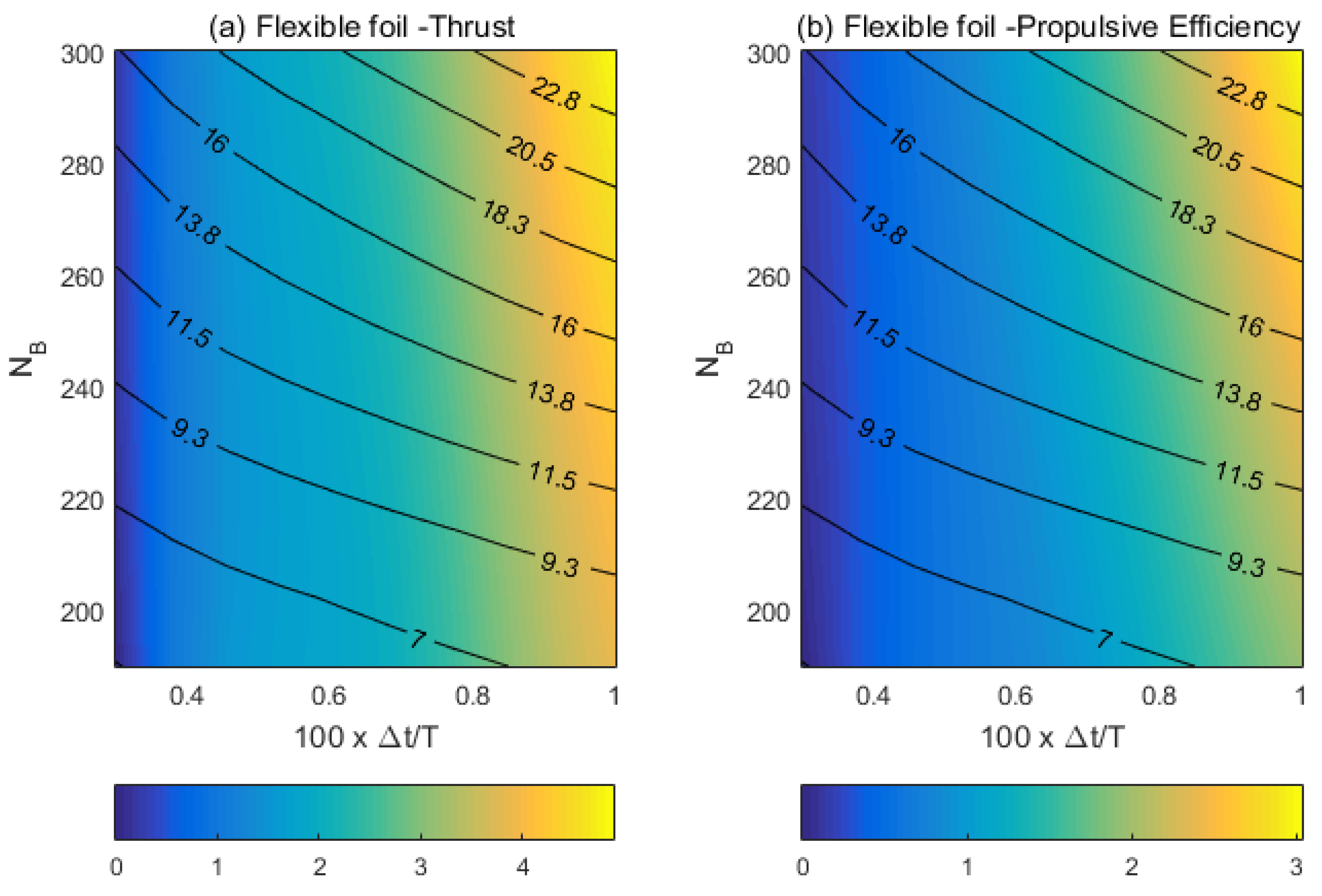
A convergence study for the case of a chord-wise flexible flapping foil is presented in
Figure 8. These simulations are obtained with the proposed coupled BEM–FEM scheme based on the Newton–Raphson iterative scheme for the fluid-flow problem. The region that corresponds to greater values of the relative error appears for simulation with a coarse discretization in time. The same behaviour is also observed for the propulsive efficiency. The iso-λ curves for the coupled BEM–FEM are not correlated to relative error minimization regions; therefore, we introduce
as a parameter constraint that is used for the numerical results that follow. In the sequel, numerical results obtained by the present model are compared against experimental measurements and data from other methods for validation.
5.2. The Case of a Flexible Flapping Foil
The effects of chord-wise flexibility on the propulsive efficiency of two-dimensional flapping foils have been investigated experimentally in [
32], showing that when properly selected, it leads to significant increase in the efficiency with small loss on thrust compared to the rigid foil. Simulations were performed for a NACA 0014 flapping foil with
and the following kinematic parameters
For the flexible foil, the thickness distribution along chord length coincides with the hydrodynamic shape of the foil, whereas the material properties correspond to relatively hard rubbers with Young’s modulus
Poisson’s ratio
and material density
.
The time history of flapping motion (pitch and heave), lift and thrust forces for both the rigid and the flexible foil are shown in
Figure 9 and
Figure 10, respectively. These results were obtained using space and time discretization
. For the case of the rigid foil in
Figure 9, the present BEM provides a very accurate prediction of the hydrodynamic forces as was expected. The experimental data in
Figure 10 are also in good agreement with the present numerical predictions in terms of the time averaged values and the overall periodic behavior of the instantaneous lift and thrust. In both cases, the proposed method predicts the maximum thrust with 1% accuracy. The differences in the peak thrust values in
Figure 10 are attributed to the non-linear structural behavior and/or viscous effects, which are not modelled. It is interesting to note here that, in this case, the maximum displacement is small and occurs at the TE of the foil. Thus, incorporating effects of chord-wise flexibility, leads to significant enhancement in propulsive efficiency with a slight decrease of the thrust coefficient.
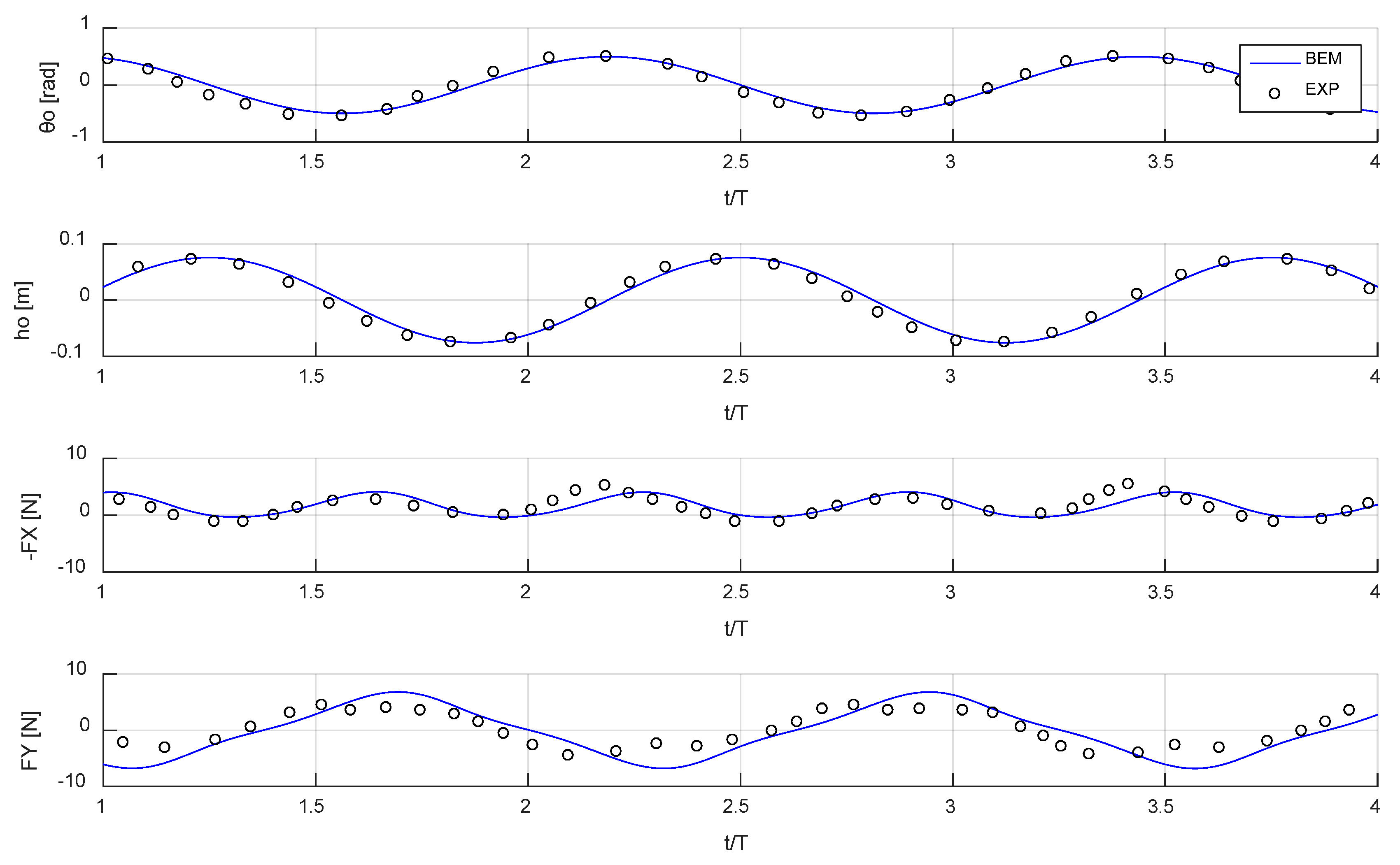
5.3. The Case of a Flexible Heaving Foil
In order to further validate the present method and illustrate its ability to capture the main hydro-elastic effects of chord-wise flexible foils, we performed another series of simulations based on the experimental work of [
34], for which case semi-analytical predictions are also available in [
35]. In the latter work, the response of flexible plates performing heaving-only motions across a range of frequencies and heaving amplitudes was experimentally studied.
In this case, a flat plate with material properties
,
is actuated at the LE with heaving amplitude
oscillating frequency within the interval
and
. For a plate immersed in fluid, see [
34], it is reported that the first resonance frequency is equal to
, whereas for the same structure in vacuo the corresponding frequency is estimated to be 14.96 rad/s.
A comparison between the present method and the experimental data from [
34] is shown in
Figure 11,
Figure 12,
Figure 13 and
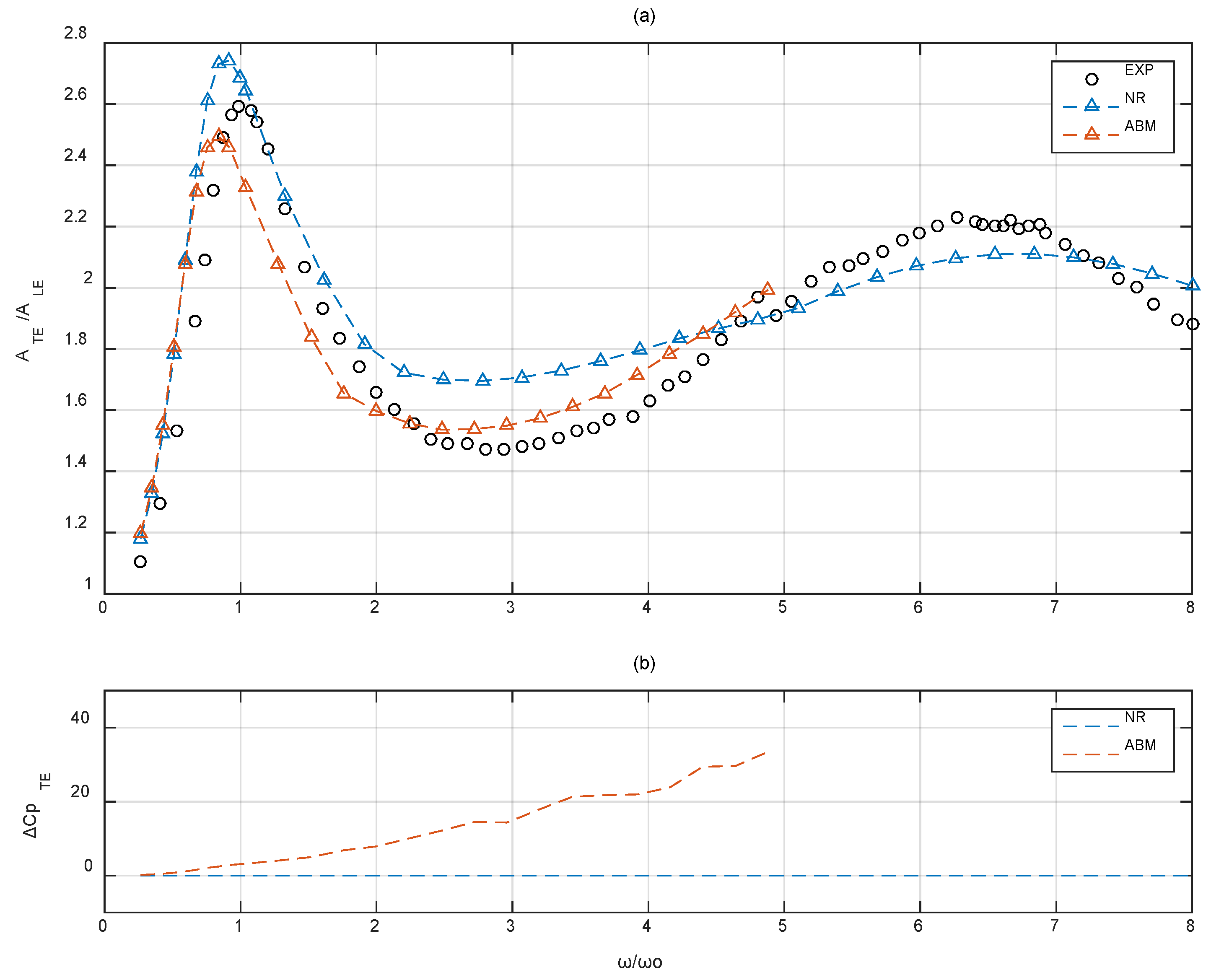
Figure 14. The trailing edge/leading edge (TE/LE) amplitude response
as a function of the non-dimensional frequency
is presented in
Figure 11a. For comparison purposes we performed simulations with both solution approaches for the hydrodynamics problem. Particularly, for the simulations performed with BEM–NR, the following space and time discretization are used:
Moreover, the damping terms (
Section 4.1.1) were tuned to
. The first coefficient (mass) affects the plate’s response near the first resonance frequency, while the second coefficient (stiffness) has a more significant role in the higher frequency regime.
It is observed that the present method, based on either the BEM–NR or BEM–ABM, displays general agreement with the experimental results, especially around the first resonant frequency. Interestingly, the BEM–ABM provides very accurate prediction up to some values. A second resonance frequency is also evident in the range of frequency examined, where the elastic response is considerably smaller. In this case, the behavior of the BEM–ABM becomes less efficient. This is due to the enforcement of the pressure-type Kutta condition concerning the pressure difference at the trailing edge. The solution scheme based on the BEM–NR satisfies exactly the pressure-type Kutta condition for all frequencies; however, the BEM–ABM despite the fine discretization used
leads to a finite pressure difference at the TE, as shown in
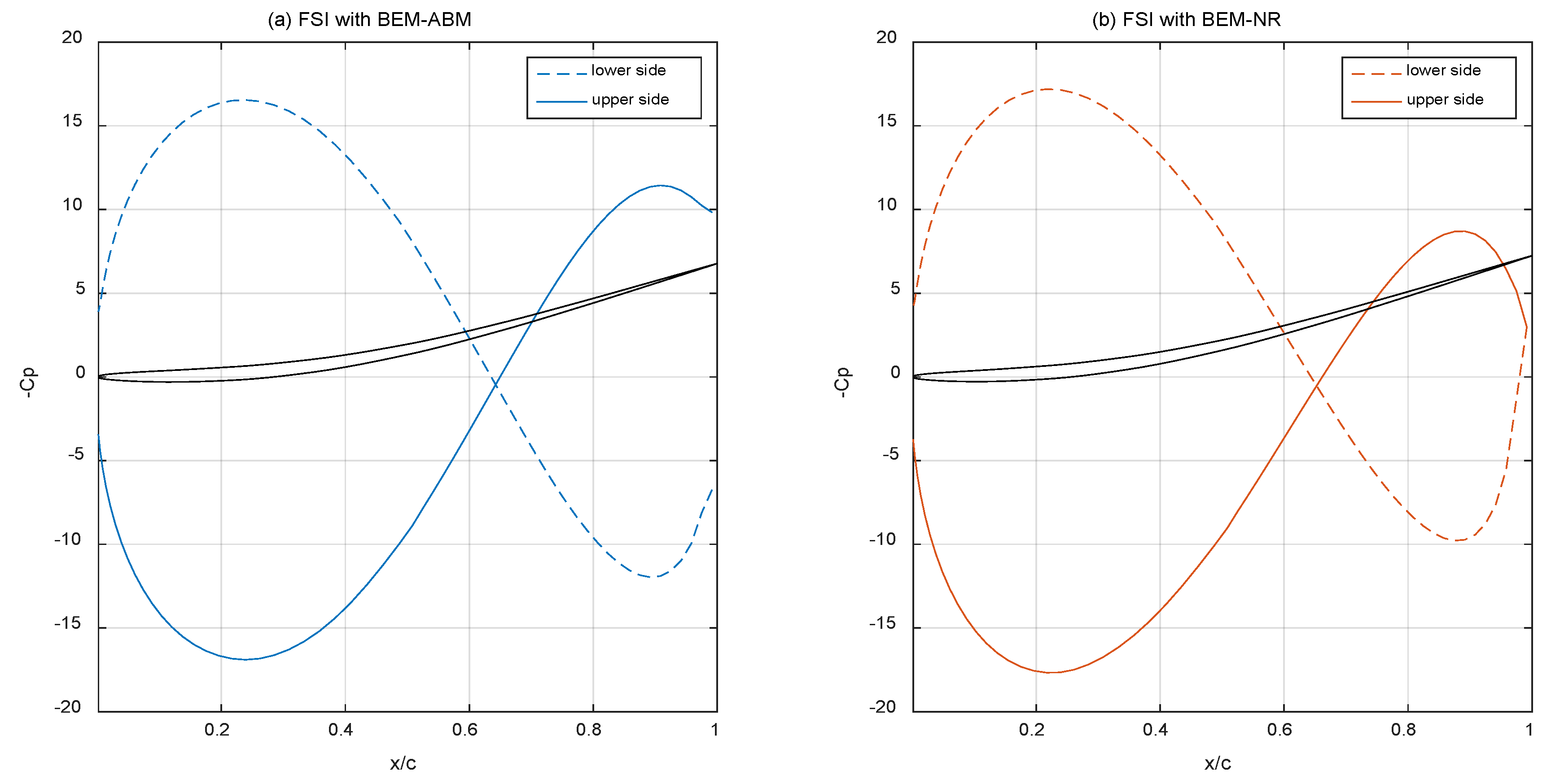
Figure 11b.
This is further illustrated in the comparison between the distribution of pressure coefficient in
Figure 2, for the case of BEM-ABM and BEM-NR. The pressure distributions are very similar, leading to compatible predictions of integrated forces and moments on the foil. However, the calculated pressure difference at the trailing edge by the BEM–ABM, affects the value of the shed vorticity and produces error in the numerical solution as the frequency increases further, see
Figure 11b.
In this example, for
, results have been obtained only by the BEM–NR model, and the second resonant peak is underestimated, a finding that agrees with similar predictions from the work by [
35], which is attributed to the inability of potential-based methods to account for viscous effects manifesting at higher frequencies. In the present work, a proportional damping is employed, and the use of a more complex damping model, see, e.g., [
27,
35], that could further improve the results is left to be examined in future work.
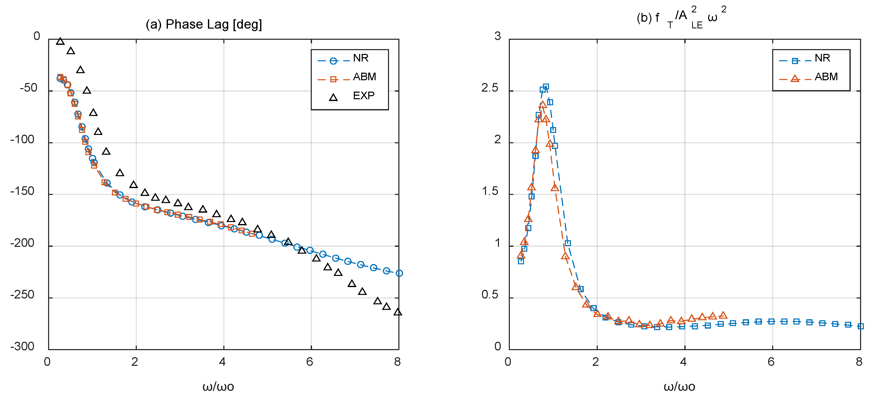
A successful comparison between the numerical model and the experimental results regarding the TE/LE phase lag, as observed in the earth-fixed reference frame, is presented in
Figure 13a. For higher values of the frequency, the error in the phase lag prediction increases. This is also the case for the TE/LE amplitude response ratio in
Figure 11a. Nevertheless, the present method predictions are still within acceptable limits. Moreover, in
Figure 13b it is shown that for thrust predictions the two solution approaches, namely the BEM-ABM and the BEM-NR, for the hydrodynamic problem are in very good agreement, justifying the hybrid time-integration numerical scheme presented in
Section 4.2.2.
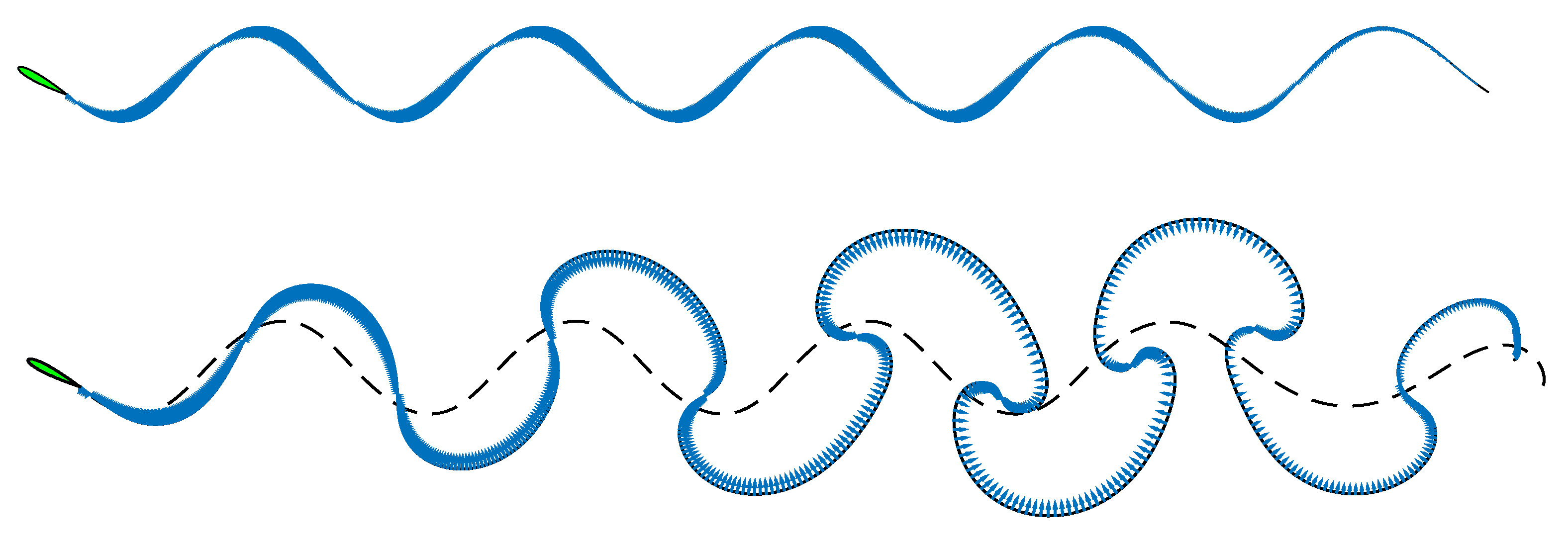
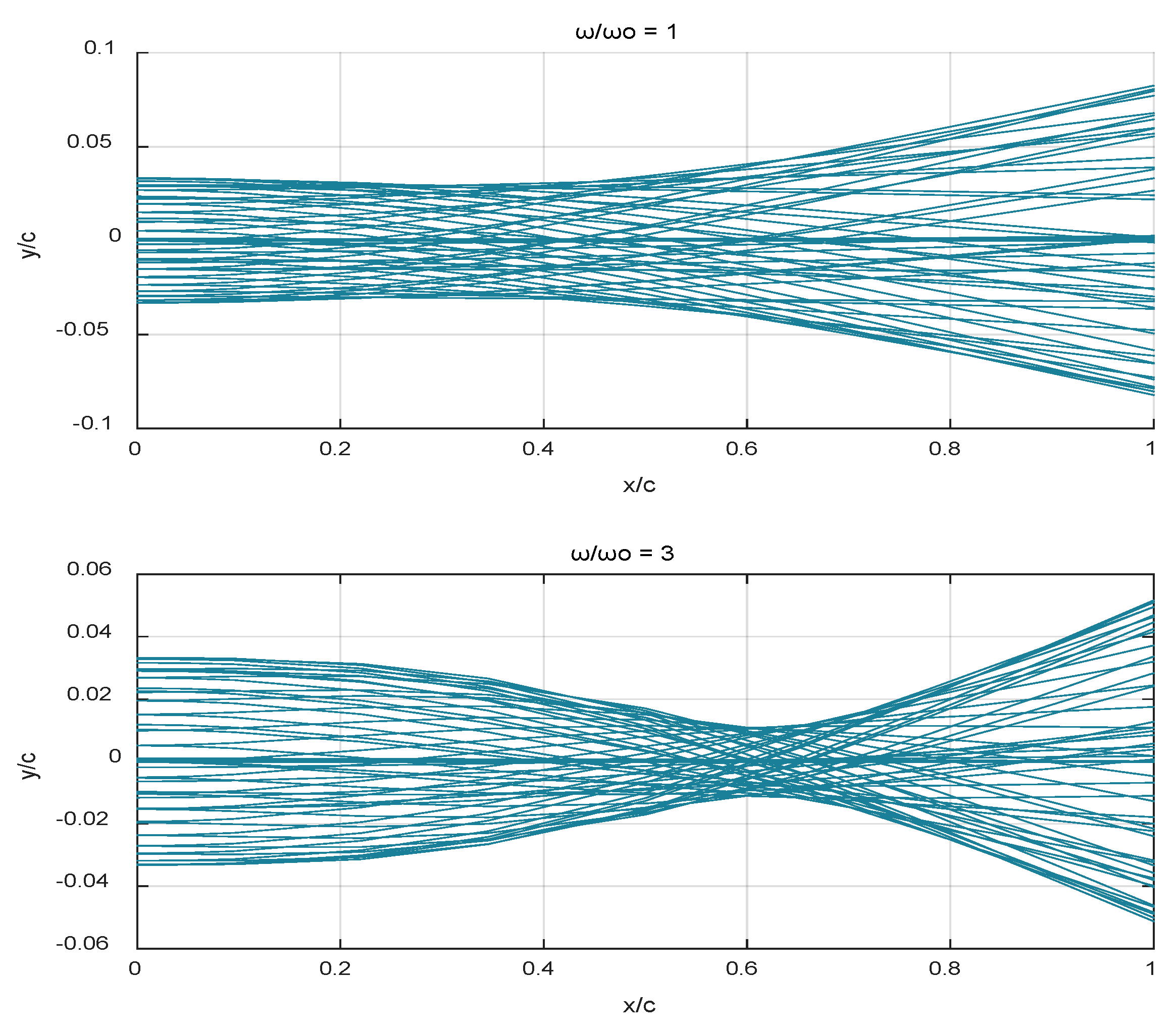
Finally, in
Figure 14, the deflection plots for time instances in a period of the heaving motion are plotted. Results are presented for two values of the non-dimensional frequency. We observe that, for
, the response of the plate displays a neck at around 2/3 of the chord due to the second plate mode excitation. These results agree well with the experimental data presented in [
34,
35].
5.4. Effects of Flexural Rigidity on Froude Efficiency
Carefully chosen flexibility characteristics have the potential to further enhance the propulsive performance of flapping-foil thrust, as has been reported in [
32] and confirmed from the simulations presented in
Section 5.2. To further investigate the effect of flexibility on Froude efficiency and thrust, additional simulations were performed, and results are shown and discussed in this section. For this study, a NACA 0012 hydrofoil with
and center of rotation at 1/3c is considered. The kinematic parameters of the flapping foil are the following
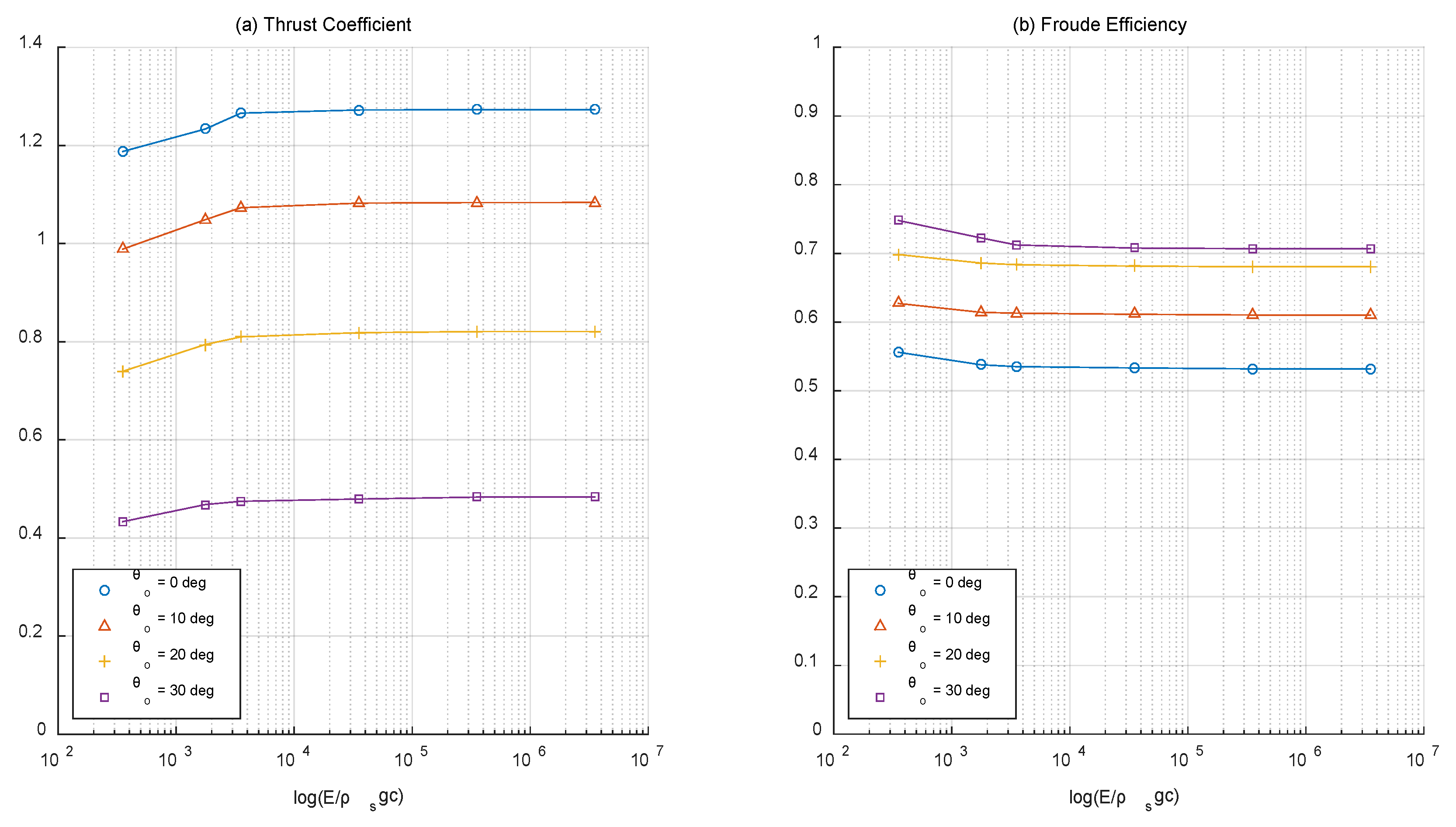
The average thrust coefficient and Froude efficiency are studied as functions of the non-dimensional flexural rigidity
for a selection of pitch amplitudes
Results are presented in
Figure 15, where it is observed that as Young’s modulus is reduced, the propulsion efficiency rises. Indeed, an efficiency increase of 6% is observed for
, as compared to the rigid case. This, however, is at the cost of thrust reduction. Especially, in cases when the kinematic parameters are not optimized, i.e., purely heaving motion, carefully choosing flexibility has the potential to enhance the propulsion efficiency considerably. Motivated by the work of [
25], we estimated the maximum effective angle of attack
for the flexible foil based on Equation (1b) with
.
For the most stiff foil with
, the estimated maximum effective angle of attacks, that correspond to
are
Typically a decreasing
leads to a decrease in thrust and an increase in efficiency for rigid foils. In that sense, the value
corresponding to zero pitching amplitude for the most flexible foil
explains the behavior of the results in
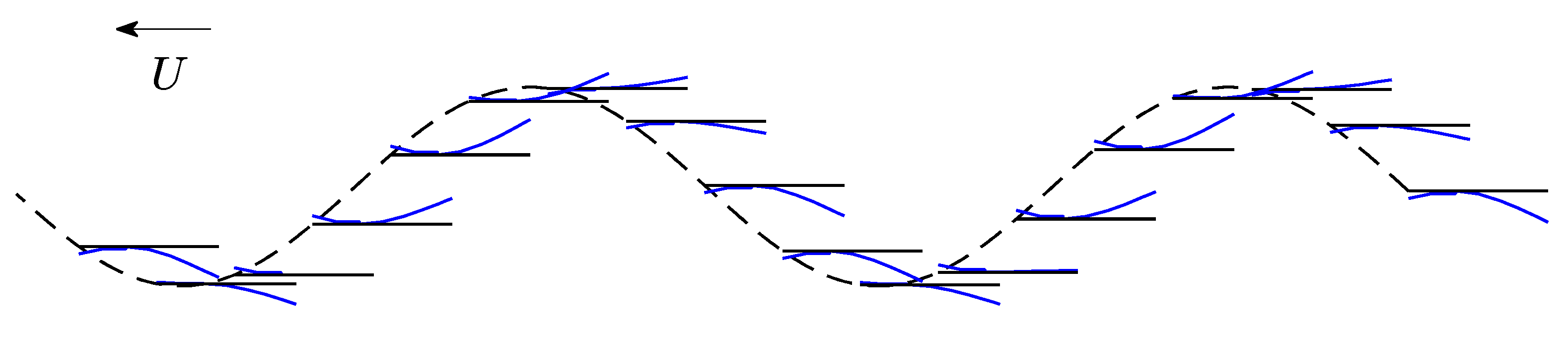
Figure 15. A qualitative explanation is also provided in
Figure 16, where typical configurations of the instantaneous curvature of the flexible foil compared to the camber line of the rigid equivalent are presented on the trajectory of the LE presented.
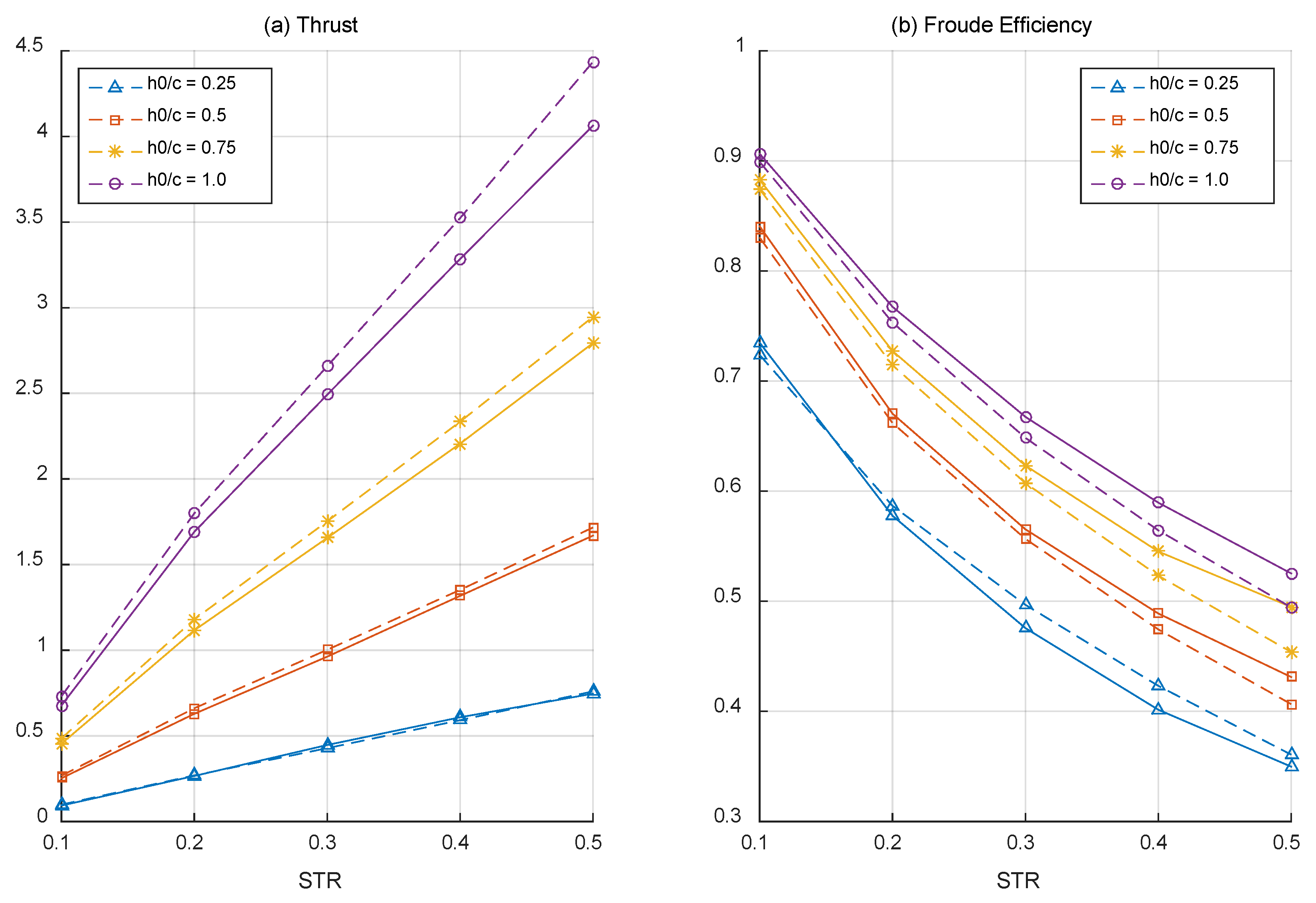
In
Figure 17, numerical results are presented to illustrate the effect of chordwise flexibility on the thrust and Froude efficiency over a range of Strouhal numbers with heaving amplitude
as a parameter. The simulations are performed for a flapping NACA 0012 hydrofoil with
and the rest of parameters:
The chosen material corresponds to one of the most elastic ones examined before, characterized by
It is clearly observed in this figure that chordwise flexibility leads to decrease of thrust as Strouhal number increases, especially for higher amplitudes of heaving motion. On the contrary, flexibility enhances the propulsive efficiency with increasing amplitude of heaving motion and higher value of Strouhal number.
6. Conclusions
Flapping foils with chord-wise flexibility were studied in this work as unsteady thrusters with enhanced propulsive performance. To investigate the hydroelasticity effects on the thrust and propulsive efficiency of such systems, a mathematical model is proposed for the FSI problem. The fluid flow modelling is based on potential theory, whereas the elastic response of the foil is based on the Kirchhoff–Love theory for thin plates under cylindrical bending. A non-linear fully coupled BEM–FEM numerical scheme is developed to simulate the time-dependent structural response of the flexible foil undergoing large prescribed general motions. The proposed iterative scheme ensures stability and convergence of the coupled numerical simulation, as proven by the convergence study shown in
Figure 6,
Figure 7 and
Figure 8. The present method is also extensively compared against experimental data for validation, demonstrating its ability to capture the main aspects of the FSI problem.
The proposed method has been successfully compared with experimental data found in [
32] for the case of a chord-wise flexible foil performing combined heaving and pitching motions; see
Figure 9 and
Figure 10. The results indicate that incorporating chord-wise flexibility in flapping-foil design could lead to 13% enhancement of propulsive efficiency, as compared to rigid foils.
The response of flexible plates performing heaving-only motions across a range of forcing frequencies and heaving amplitudes, found in the experimental work of [
34], has also been studied for comparison purposes. These numerical results were in good agreement with the experimental measurements for various aspects of the non-linear dynamic system; see
Figure 11,
Figure 12,
Figure 13 and
Figure 14. The present method is shown to satisfactorily predict both the TE/LE amplitude response as a function of the oscillating frequency, see
Figure 11a, and the phase lag between the LE and TE as reported during the experiments; see
Figure 13a. The first and second resonant frequencies were quite accurately predicted; however, our model slightly underestimates the TE amplitude response near the second resonance. Furthermore, the envelopes of the foil’s elastic deflection, see
Figure 14, agree with the predictions presented in the work of [
35]. In that sense, the non-linear BEM–FEM scheme is shown to successfully predict the hydrodynamic loads as well as the fluid-driven deformation of flexible flapping foils with general thickness profile and flexural rigidity.
Motivated by the propulsive performance enhancement offered by flexible foil-thrusters, we performed parametric studies, see
Figure 15 and
Figure 17, in order to further investigate the effects of elasticity over a range of design parameters, including Strouhal number, heaving and pitching amplitudes. The results illustrate that chord-wise flexibility and flexural rigidity profile variations can significantly improve the propulsive efficiency of the biomimetic thruster. Particularly, it is shown in
Figure 15 that as flexural rigidity is reduced, the propulsion efficiency rises, leading to an efficiency increase as large as 6% observed for
, as compared to the rigid case. This, however, is obtained at the cost of thrust reduction. The results in
Figure 17 illustrate that chord-wise flexibility leads to a more pronounced decrease in the thrust as Strouhal number increases, especially for higher amplitudes of heaving motion. On the contrary, flexibility enhances the propulsive efficiency for high amplitudes of heaving motion and Strouhal numbers.
To conclude, future work is planned towards the detailed investigation and systematic examination of the structural response of the flexible foil over a range of design and operation parameters, including flexural rigidity profiles inspired by nature. Additional comparisons and benchmark studies between the present non-viscous BEM–FEM scheme and high-fidelity viscous CFD solvers is also left for future work. Direct extensions include modelling various nonlinearities associated with large deflections and viscous effects [
37,
53]. Another aspect concerns the code optimization using GPGPU programming and message passing interface (MPI) techniques to significantly reduce computational time and cost, see, e.g., [
13,
38,
44]. This step will allow three-dimensional modelling as well as shape and material optimization, supporting applications concerning realistic designs. Finally, the present method could also find useful application to calculate the flexibility effects on the performance of novel marine renewable energy devices based on oscillating foils; see [
13].


