Abstract
A biomimetic semi-activated oscillating-foil device with multiple foils in a parallel configuration is studied for the extraction of marine renewable energy. For the present investigation, an unsteady boundary element method (BEM) is used for the simulation of 3D lifting flows. For this work, the device is assumed to be submerged far from the free surface and the sea bottom. However, the geometry of the body and the initial shape of the wake are general. For the numerical simulations, a high performance in-house GPU-accelerated code (GPU-BEM) is developed. For the calculation of singular integrals, an adaptive algorithm based on the Gauss–Lobatto quadrature is used. Concerning the numerical scheme of GPU-BEM, the convergence of the method was tested, the numerical characteristics were determined and the method was validated. A parametric study of a single-foil device is presented to determine the performance characteristics of such devices. Next, twin-foil devices are investigated in parallel and staggered configurations with a phase difference between the two foils. Finally, the multiple-foil parallel configuration is compared against turbines. After enhancement and further verification, the present method is proposed for the design and control of such biomimetic devices for the extraction of energy from waves and tidal currents nearshore.
1. Introduction
The marine environment has abundant resources of renewable energy, and in recent years, their exploitation has become the subject of an increasing number of studies. For the extraction of tidal energy, various designs have been proposed, i.e., turbines, systems based on vortex-induced vibrations, piezoelectric devices, sails and oscillating foils [1]. The majority of these designs and proof-of-concept studies belong to the category of horizontal axis turbines [1].
In the present study, we consider oscillating foils for marine energy extraction. Apart from this mode of operation, foils performing flapping motion are also studied as efficient propulsion systems. Research and development of flapping wings is supported by extensive experimental, theoretical and numerical studies, with results that show that in optimal conditions, such systems can achieve high thrust levels (see, e.g., [2,3,4]). Flapping wings can also be used as “thrust augmentation devices” fitted on the hulls of ships. In this case, the ship’s motion with waves can provide one mode of oscillatory motion, free of cost. As a result, these devices have gained popularity as secondary propulsion systems. References [5,6,7,8,9,10,11,12,13] provide detailed analysis of the characteristics of such systems. Also, some of the present authors were involved in the research project BIO-PROPSHIP [14] for the investigation of flapping foils.
Foils can also be used as devices that convert tidal stream energy to other forms, i.e., electricity. In tidal energy harvesting mode, oscillating foils operate by absorbing energy from the incident current. One of the first reports on such designs is that of reference [15], and some early experiments were conducted in 1982 [16].
Oscillating foils combine a pitch motion and a heave motion. In reference [17], oscillating-foil devices are classified into three categories depending on the activation mechanism of the oscillating foil. First, there are fully activated foils, where both the pitch and heave motions are prescribed. Second, there are semi-activated foils, where the pitch motion is given as input and the heave is the response to the hydrodynamic forces. Third, there are fully passive foils, where both motions are driven by the forces acting on the foil. In the present work, we study the semi-activated oscillating foil, because this alternative is a more feasible design than the fully activated system and it provides a mechanism to actively control the operation of the foils, in contrast to the fully passive design. Also, energy extraction of both waves and current is studied by the authors in [18].
Moreover, efforts have been made to map the performance of oscillating foils in the energy extraction regime, i.e., parametric studies [19,20,21]. The basic parameters of the harmonic pitching motion have been mainly investigated, through experiments or numerical simulations. In [19], the authors report a power-extraction efficiency of 36.4% for a pitching amplitude of 76.3 degrees, using the FLUENT commercial software.
Various studies have shown that oscillating foils can have advantages over tidal turbines. More specifically, the power extraction of horizontal turbines is limited by the Betz limit, and the theoretical maximum power that these systems can extract is 59.3% of the power available in the water passing through the disk swept by the turbine [22]. On the other hand, in a few research works, it is stated that devices based on oscillating foils can surpass the Betz limit (see, e.g., [23,24]). This can be explained by oscillating foils using the unsteadiness of flow and vortex dynamics to their advantage, enhancing the performance of the device.
Oscillating foils can also take advantage of leading edge vortices (LEVs). LEVs can help improve the energy extraction capabilities of the system. In reference [25], it is shown that appropriate vortex control mechanisms can help the device to recover energy from the disturbed flow by generating a low-pressure region at the upper surface of the foil near the trailing edge.
Moreover, oscillating foils can operate near the sea surface, allowing the device to extract energy from both tidal streams and waves. Conservative numerical studies (small pitching angles) show that oscillating foils operating nearshore under the influence of both waves and sheared currents demonstrate an enhanced performance index of 53.5% [18], also exploiting wave energy.
Furthermore, oscillating-foil devices with two or more foils have become the subject of study by many researchers. In the simplest case, twin-oscillating-foil designs can be in either parallel or tandem configuration. Due to the nature of oscillating foils, both configurations have advantages. In a parallel configuration, the foils take advantage of the "ground effect", that is, the flow is constricted between two foils when the distance between them becomes small, increasing the lift force. In a tandem configuration, the foils are placed one behind the other, with the foil downstream interacting with the wake of the upstream foil. In this configuration, vortices shed by the upstream foil can interact strongly with the downstream foil, and, under the correct choice of the distance and phase difference between the two foils, the instantaneous performance can be increased by a local rise of the available dynamic pressure [26]. In both configurations, the performance of the device is enhanced.
Therefore, another advantage of oscillating foils over turbines, when considering arrays of devices, is that oscillating foils can surpass tidal turbines in terms of performance. Two oscillating foils in a tandem configuration have 59.9% efficiency [26] and can reach values higher than 90% for 15 foils [27]. Meanwhile, turbine arrays in similar configurations show efficiencies that asymptotically reach 66% [24]. Multi-foil parallel configurations for power extraction have been studied both experimentally and numerically in [28,29]. The authors found that in the anti-phase case (phase difference of 180 deg), the wing distance plays a major role in increasing the performance of the foil, and they reported a 25–33% increase in performance for a 10-wing configuration with an adjacent wing distance of 2–2.5 chord lengths.
In the present work, we study a semi-activated oscillating foil device. For this reason, 3D simulations are performed in order to obtain data for a parametric study. The oscillator parameters (frequency and damping coefficient) and geometric parameters (planform shape) are investigated for a single foil in order to find the optimal configuration. Next, multi-foil devices are studied. The main purpose of this paper is to illustrate the effect that various design parameters have on the performance of the oscillating-foil device, as an alternative to tidal turbines.
In reference [7], an in-house GPU-accelerated boundary element method (GPU-BEM) was developed for 3D lifting flows around foils operating beneath the free surface and in non-linear waves. For the following numerical simulations, GPU-BEM is extended for the treatment of the semi-activated foil. The code takes advantage of advanced parallel programming techniques and general purpose programming on graphics processing units (GPGPU), by using the CUDA C/C++ application programming interface. GPGPU was chosen as it provides massive parallelization capabilities even on a single computer, allowing for fast simulations and efficient usage of the computational resources provided by a modern computer.
The rest of the paper is organized as follows. In Section 2, we present the hydrodynamic modeling of the oscillating-foil device with one or multiple foils. In Section 3, we provide a brief discussion of the decisions concerning the developed GPU-BEM software. Next, in Section 4, we present an extensive numerical investigation and discussion of the device performance in the case of single and multi-component foil arrangements. Also, the oscillating-foil alternative is compared to conventional tidal turbine devices.
2. Mathematical Formulation
In this section, we present the mathematical foundation of the method used in the present work to study oscillating foils. The problem consists of two sub-problems: the lifting-flow initial boundary value problem (IBVP) and the oscillator initial value problem (IVP). The oscillation is driven by the lifting force, resulting from the solution of the IBVP. Also, the hydrodynamic problem depends on the state of the oscillator. Thus, the two problems are not independent and a coupling algorithm is needed.
In Section 2.1, we present the modeling of the semi-activated system with one or multiple foils. Next, in Section 2.2 and Section 2.3, we discuss the hydrodynamic problem and the numerical scheme used for the solution of the IBVP. In Section 2.4, we present the adaptive integration quadrature used in the present work. Finally, in Section 2.5, we present the coupling algorithm between the IVP and the IBVP, providing a time integration scheme.
2.1. Oscillators
In the present work, multiple-foil configurations are considered. In the case of a single foil, the free heaving motion of the semi-activated device with prescribed pitching motion is modeled by a one-degree-of-freedom damped oscillator, described by the following equation:
where h is the heave of the foil, is the mass of the foil, is the damping coefficient, modeling the power take-off, is a spring coefficient, representing the elastic mount, and is the lift generated by the oscillating foil (see Figure 1). As mentioned earlier, the lift force depends on the heave position () and the time derivative (), introducing an implicit non-linearity to the problem. For the sake of simplicity, in the sequel we write .
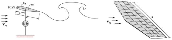
Figure 1.
Schematic of the semi-activated flapping foil marine energy extracting device. The foil is attached to a power take-off (PTO) modeled by a damper and a spring.
The rotational (pitching) motion is prescribed and performed about a pivot axis located at distance from the leading edge (LE). In the present work, the prescribed pitch angle of the foil () is chosen to have a sinusoidal profile
where is the amplitude of the pitching motion, and is the angular frequency. The examination of more general pitching angle profiles, including active control of the rotation, to further increase the power output of the device, is left as a subject of future work.
In the case of multiple foils in parallel configuration, the foils are placed so that their mean positions are spaced by a distance () in the vertical direction (see Figure 2). In this case, the odd-numbered foils are joined together in order to move in the same way, and the same is true for the even-numbered ones. Then, the equations of motion for the two groups of foils are
where the subscripts E and O denote the even-numbered and the odd-numbered foil groups, respectively. The lift forces on the right-hand side of Equation (3) are the sum of all the lift forces of the foils in the group
where and are the number of foils in the even and odd groups, respectively. Now, the parameters , and refer to the entire foil group. For the results presented in the next section, it is assumed that these parameters are multiples of the number of foils in each group, i.e.,

Figure 2.
Schematic of the proposed multiple-foil configuration. Each group of foils is attached to a PTO.
The pitch motions of the foils of each group are given by Equation (2) but differ in phase
where and are the phases of the two pitch motions. For the sake of simplicity, will be assumed to be zero.
In order to sustain the pitch motion, the device consumes power given by the sum of the power consumptions of the individual foils, as follows:
where is the hydrodynamic moment in the direction of the pivot axis. The power generated by the device is given by the following relation:
Then, the period-averaged net power generated by the device is
The performance of the device is measured by the following performance index:
where is the total cross sectional area swept by the foils in a period, and is the density of the fluid. The denominator in the above relation represents the hydrokinetic power flux of the current flow through the area of the fluid swept by the foils. In order to calculate the performance index of the studied device, the cross sectional area swept by the vertical motion of the foil(s) is calculated. In particular, having obtained the solution of the problem, the heaving motion of the foil(s) and the prescribed pitching motion of the foil(s) are known. Using the latter results, the cross sectional area swept by the foil(s) is calculated by considering two approaches, as follows:
- (i)
- only the vertical motion of the pivot axis of the foil(s),
- (ii)
- the maximum deviation in the vertical direction of the edges of the foils (which also includes the effect of the pitching motion of the foils).
Subsequently, the performance index of the system is obtained by dividing the mean net power generated by the device in a period by the hydrokinetic power of the current flow through the above cross sectional area; a comparison of the two estimations for a particular set-up is presented and discussed in Section 4.1.
2.2. Hydrodynamic Problem
In this subsection, we present the methodology used to obtain the lift force of the foils. To calculate the hydrodynamic forces, the boundary element method (BEM) is used. The model is based on the potential flow theory, the solution is obtained using the theory of boundary integral equations (BIE), and the numerical treatment is performed using BEM. In the present work, the following assumptions are made concerning the hydrodynamic model (see also Figure 1):
- The device is assumed to operate submerged in an unbounded domain (), ignoring the free-surface and bottom boundaries.
- The flow is assumed to be irrotational and incompressible in .
- The rotational part of the flow is restricted in the trailing vortex sheets emanating from the trailing edge (TE).
- The Morino-type Kutta condition is applied, ensuring the continuity of the potential jump through the TE.
The potential flow is defined by the Laplace equation
where is the disturbance potential field. On the foil surface (), the no-entrance boundary condition is satisfied
where is the gradient of a function in the direction of vector , is the net velocity vector of the foil surface due to the heaving and pitching motions, and are the direction and the position of the pivot axis, respectively, is the translatory velocity of the foil on the earth-fixed reference frame, and is the unit normal vector to the boundary surface. Moreover, is the current velocity vector that can model weakly rotational fields lying in the background.
We treat the above as an initial boundary value problem, and we assume that the disturbance potential and its derivatives vanish at a large distance from the foil.
The wake () of the hydrofoil is modeled as a free shear layer surface. On this surface, the kinematic and dynamic boundary conditions [30] are imposed as follows:
In the equations above, we denote with the superscript “+” the upper side of the wake and with the superscript “–“ the lower side. These conditions, together with the approximate Bernoulli-type equation for weakly rotational flows [7]
result to
where is the potential jump through the wake boundary and is the material derivative based on the mean total velocity of the wake . Here, it should be noted that the shear surface should move and deform according to the total velocity of the flow, including both the current velocity and the disturbance velocity due to the operation of the foil. In the present work, we omit the second component and the dynamics of the wake are linearized. However, the wake shape is not prescribed due to the unknown heaving motion and is obtained as part of the solution. At a far enough distance from the foil, the disturbance field vanishes.
Finally, in order to model the circulation around the foil and ensure continuity of pressure on the sharp trailing edge, one more condition is needed, named the pressure-Kutta condition. Here, a Morino-type Kutta condition is used, demanding continuity of the potential jump at the trailing edge, as follows:
where here is the dipole intensity generated at the trailing edge and transferred to the wake at any given time.
2.3. Boundary Integral Equation and Discretization
Using Green’s formula for the problem described in the previous subsection and for points on the foil surface, we obtain the following boundary integral equation (BIE) for the potential () on the foil and its normal to the surface derivative ()
where is the fundamental solution of the 3D Laplace equation
where is the distance between points . The function G represents the potential by a point source at point To discretize Equation (18), the foil and wake surfaces are approximated by using a bilinear quadrilateral boundary, which ensure global continuity of the geometry and no gaps between elements (see Figure 3). Moreover, the potential and its normal derivative are assumed to be constant over each element, and a collocation scheme is used to satisfy Equation (18) at the centroids of the elements on the foil surface. Furthermore, the Morino-type Kutta condition is satisfied on the collocation points of the first row of boundary elements in the wake after the trailing edge of the foil. For this purpose, a standard wake model is used, as presented in the close-up detail in Figure 3, where the starting part of the geometry of the trailing vortex sheet is defined as the extension of the bisector of the trailing edge angle, and subsequently it is approximated by the surface generated by the history of the oscillatory motion of the trailing edge, in conjunction with translation in the downstream direction with the parallel inflow velocity (see [7,31]). The discretized Morino-type Kutta condition is
where the subscripts and denote the points adjoined to the trailing edge on the upper and lower side, respectively. The discrete subsystem modeling the hydrodynamics (BIE and Morino condition) is as follows:
where and are the induction factors of source and dipole distributions, respectively;

Figure 3.
Foil and wake model geometry discretization. The foil and wake boundaries are approximated with bilinear elements. The source and dipole distribution on the foil is considered piecewise constant. The detail shows the wake model geometry in the vicinity of the trailing edge.
The disturbance velocity tangent to the foil surface is then calculated by a second-order curvilinear finite difference scheme [7]. The total velocity field on the foil surface can be found by adding the disturbance velocity with the Neumann data. Next, the pressure on the foil surface can be found by using Equation (15).
In the case of multi-foil configurations, matrices A and B contain the factors of all the foils, including the induction terms from an element of one foil (and its wake) to a point on another foil.
2.4. Adaptive Integration Method
Some of the surface integrals arising in BEM (Equation (22)) are singular because there exists a collocation point that coincides with a point on the integration domain. For this reason, an adaptive integration algorithm is developed to facilitate the calculation of integrals. In adaptive integration methods, the interval of integration is dynamically refined in order to achieve a better approximation near the singular points. More specifically, a simple quadrature is used to obtain a first estimate of the integral, in the integration domain () and, next, the interval is partitioned to m subintervals and the simple quadrature is subsequently used on each subinterval. Then, the first estimation is compared to the sum of the subinterval estimations to determine the convergence. This procedure is repeated on every subinterval until a convergence criterion is satisfied.
The method relies on recursively integrating the function on smaller subdivisions of the initial domain. In reference [32], an adaptive quadrature based on the simple Simpson’s (1-4-1) rule is studied. The author proposed an accurate convergence criterion and modified the quadrature to include a term for convergence acceleration. Moreover, in reference [7], this method was exploited for the calculation of the singular integrals that appear in the proposed GPU-BEM. In reference [33], an adaptive quadrature based on the four-point Gauss–Lobatto rule with two successive Kronrod extensions is presented.
In the present work, we propose an adaptive algorithm based on an N-point Gauss–Lobatto quadrature with a uniform m-division strategy (). The simple quadrature rule used is defined as follows (see [34]):
where the weights are calculated by the following formula:
and is the Legendre polynomial of order N, and the nodes are the root of the first derivative of . For the purpose of the present work, the necessary nodes and weights are pre-calculated, following the procedure found in [35]. The error of is (see also [34], p. 888)
The Richardson extrapolation technique [36] is used to increase the convergence rate of the recursive algorithm. For the Gauss–Lobatto quadrature of order , the error of the approximation is , where here denotes the integration interval length, and for the adaptive routine, with m uniform subdivisions at each recursion level, the convergence can be accelerated by applying the Richardson extrapolation as
where is the final accelerated estimation of the integral and is the non-accelerated result. In the relation above, the arguments and of are the subdivision lengths for the current and the previous recursions, respectively. The termination criterion in the case of is
where is the desired error margin for the integration.
To evaluate singular surface integrals, it is important to have a very good approximation of the inner integral that bears the singularity. Then, the outer integration can be done by a lower order routine. In this way, the benefits of accuracy and robustness of the high order routine used for the inner integration are combined with the great speed of the simpler routine of the outer integration. Finally, a fast and elegant routine for evaluating singular surface integrals is produced by using object-oriented programming.
Here, it should be noted that the proposed adaptive routine can be generalized for integration over N-dimensional domains. An N-dimensional integration can be viewed as an integrant function. In computer programming terms, it can be considered as a functor object. A functor corresponding to an integration in N-1 dimensions can be passed as an integrant to the integration routine, resulting in the functor corresponding to the integration in N dimensions. This can be applied recursively for all the dimensions and then, when the outermost integral is evaluated, we gain the result of the initial N-dimensional integral.
2.5. Time Integration and Coupling Scheme
By setting
we can reduce the order of the oscillator equations (Equations (1) and (3)) as follows:
The above equation is discretized in time by applying a Crank–Nicolson scheme. Therefore, the relation above is approximated as follows:
or
This nonlinear system of equations is then solved using Newton’s method, as follows:
where is the Jacobian matrix of system approximated using second-order central differences. As already discussed in the previous sections, the main difficulty of the problem is that it is strongly coupled since the foil lift force is strongly dependent on the heaving motion and its time derivative. Thus, iterations are necessary to treat the non-linear fluid-structure couplings. More specifically, the dynamical system is integrated in time using the Crank–Nicolson scheme, Equation (30), based on a time step appropriately selected to ensure stability and accuracy. An internal loop of iterations is needed at each time step (indicated by using small n-index in Equations (31) and (32)) in order to ensure the dynamical equilibrium between fluid pressure forces and inertia forces and between spring and damping forces. This is succeeded by applying Newton’s method, Equations (31) and (32), where the Jacobian of the system is evaluated by solving the hydrodynamical subproblem at each internal iteration.
3. Software Implementation
BEM is a massively parallelizable method because the calculation of the induction factor for each term and can be performed independently, i.e., without inter-thread communication. This results in a significant reduction of the calculation time, by splitting the workload on multiple threads. Moreover, due to the reduction of dimension of the problem, BEM requires less memory compared to methods based on the discretization of the entire computational domain. Therefore, parallelization on a GPU platform, where memory resources are limited, is suitable for the present method. For GPU parallelization, the CUDA API is chosen, as it offers higher performance on NVIDIA GPUs than the alternatives. The most computationally intensive operations are the calculation of the induction factors and the solution of the linear system for the calculation of the disturbance potential on collocation points. For the solution of the system, the LU solver offered by the cuBLAS library is used. Moreover, in order to increase the performance of the computational code further, mixed precision arithmetic is adopted. The above characteristics along with the use of the object-oriented paradigm result in an elegant, inclusive and easily extendable software. In the following subsections, some interesting aspects of the software implementation are discussed. In the present work, all the simulations were performed on an NVIDIA GTX650 Ti Boost GPU and an Intel i5-4670 3.4GHz CPU.
3.1. Mixed Precision
Most commercially available GPUs have more single-precision throughput (FP32) than double-precision throughput (FP64); e.g., the NVidia Pascal architecture SM has an FP32-to-FP64 performance ratio of 32. For this reason, single-precision arithmetic is preferred for intensive calculations.
However, in some cases single precision may introduce significant arithmetic errors, lowering the accuracy of the method. In the case of BEM, it was found in [7] that single-layer self-induction integral terms require double precision, and therefore a mixed-precision scheme is used (see also [37]). The results can then be converted to single precision for storage, and the linear system is solved with single-precision arithmetic. For example, the addition of mixed-precision arithmetic resulted in a six-fold increase in performance for 4000 degrees-of-freedom (DoFs), while the error increased only slightly but remained within the acceptable limits.
3.2. GPU Code Performance
As mentioned earlier, the two operations that consume the most computational time are the calculation of induction factors and the solution of the final linear system. As the cuBLAS library is used for the solution of the system, attention was given to the calculation of the induction factors. For increasing the performance of the software, two approaches were used. First, the code was optimized for the GPU architecture. For that, appropriate data structures were used for better memory coallescence and the CPU/GPU communication was minimized. As a result, the occupancy of the GPU was maximized. In this way, only the workload would impact the performance. Second, in order to reduce the number of calculations needed, a semi-analytical approach was adopted for the calculation of the induction factors. In the present work, the inner integration of the self-induction factors is performed by an analytical formula. For this reason, these terms are calculated separately from the rest of the elements of matrices A and B. The workload and the memory demands of the code can be further decreased by implementing the fast multipole method [38].
The performance of the final GPU parallelized code was 180 times greater than the performance of the single-threaded CPU code.
4. Numerical Results
In this section, we study the oscillating-foil device in a multi-component configuration. First, we present the convergence of the method for the spatiotemporal discretization parameters and validation through comparison with experimental results. For this, we consider a single-foil device and, next, we conduct a parametric study for this case. Also, for the case of a single foil, we examine the effect of the planform. Following, we investigate a twin-foil device in parallel and staggered configurations. We conclude the study with a comparison of the oscillating-foil design, with up to three foils, with tidal turbines.
4.1. Convergence and Validation
Before we proceed to the investigation of the oscillating-foil system, we demonstrate the convergence of the method with respect to the density of the spatiotemporal grid. The two spatial discretization parameters are the number of elements in the spanwise direction () and the chordwise direction (), and the convergence of the method in terms of the performance index of the device can be seen in Table 1. The third parameter is the size of the timestep (), considered as a fraction of the period of the oscillating motion (Table 2). For the results shown in Table 1 and Table 2, the parameters of the device are: A NACA0012 rectangular foil with aspect ratio , , reduced frequency and pitch amplitude . The non-dimensional damping coefficient is , while the spring constant and the mass of the foil are neglected. The mass is assumed to be zero, as the added mass due to the interaction with the water is far greater, meaning that the mass has little effect on the results and can be ignored [39]. In the following subsections, the parameters are kept the same, unless specified. For , , the method presents a 1.5% error compared to the most refined case (see Table 1) and so, these values will be used for the following simulations, along with .

Table 1.
Convergence of for .
Table 2.
Convergence of for , .
Next, the present method is compared with the experiments of [20] for validation purposes. In the device used in their experiments, the hydrodynamic forces were translated to a torque on a rotating shaft, by means of a swinging arm. In this case, the foil has and , the pivot axis is located at and the length of the swinging arm is . The current velocity is , the damping coefficient is and there is no elastic connection (). Here, it should be noted that end-plates were used in the experiment in order to increase the efficiency, and for this reason, in the numerical simulations an aspect ratio was used to compensate for the effect of the end-plates.
The heaving response of the foil for various values of the pitch amplitude , in the case , is shown in Figure 4. In general, the present method’s results are found to be in good agreement with the experimental data. Some minor discrepancies are observed for relatively higher values of the pitch amplitude between . The latter are attributed to the approximate Morino-type Kutta condition used in the present analysis, in conjunction with the linearized trailing vorticity dynamics associated with the simplified wake model. More accurate predictions could be obtained by using a pressure-type Kutta condition and fully non-linear wake model, and such an extension is left for future work.

Figure 4.
Heave amplitude comparison between the present method and the experiments conducted by Huxham et al. [20] for reduced frequency .
As mentioned above, in the experiment by Huxham et al. [20], end-plates were used at the tips of the oscillating wing, in order make the flow around the foil more close to being two-dimensional and to increase the efficiency of the system by reducing the downwash 3D effects. In order for the present method, where no-end plates are considered in the studied configuration, to simulate the experiment, an increased value of the aspect ratio needs to be considered (see also [40]). In such a case, the present method’s results can be compared with the measured data converted in the form of torque and net power output per unit span. Such a comparison is presented in Figure 5 by using the present method with foils of and . For reference, results obtained using the experiment aspect ratio are also plotted in the same figure using cyan solid lines. It is seen that the present method’s predictions after the elimination of the finite span effects compare well with the corresponding experimental data.
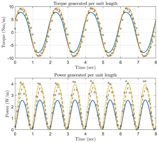
Figure 5.
Torque output and power output timeseries between the present method and the experiments of [20] for , and . Crosses denote the experimental data, solid lines denote the results of the present method with , dashed lines denote the results for , and dash-dot lines are the results for .
4.2. Parametric Study of a Single Foil
In this subsection, a parametric study of the single-oscillating-foil device is performed. In total, the effect of six parameters was examined, four related to the oscillation and two related to the geometry of the foil. Concerning the oscillation, the frequency, the damping coefficient, the pitching amplitude and the location of the pivot axis were studied. Concerning the geometry of the foil, the spanwise distribution of the chord length and a sweep angle were selected as the two parameters that define the shape of the planform.
Before continuing to the parametric study, it is useful to choose the appropriate measure for the performance. In the relevant bibliography, there are two definitions for the performance of the device. The difference between the two concerns the cross section area normal to the velocity of the current swept by the foil considered. The first definition uses the area swept by the pivot axis, while the second takes into account the whole movement of the foil, including the pitching motion. The difference between the two can be significant, especially when high pitch amplitudes are considered (see Figure 6). Another piece of information that can be extracted from Figure 6 is that the efficiency of the device increases linearly with the pitch amplitude. This result is also observed by other researchers, i.e., [18,39]. In the same figure, data from [39] are also plotted for comparison. In the sequel, the second definition of the performance index is adopted, as it produces a more realistic result and allows comparison with other types of devices for tidal energy extraction, i.e., tidal turbines.

Figure 6.
Effect of pitch amplitude on the efficiency of the device for , and . The efficiency rises linearly with the pitch amplitude. The dashed line represents the results of [39], the line with crosses represents the results of the present method with efficiency defined by the plunging amplitude, and the line with diamonds shows the efficiency calculated by including the pitching motion.
Concerning the study of the oscillation parameters, the chord, the aspect ratio of the foil and the pitch amplitude are kept constant (, and ) and the current velocity is . In Figure 7, the performance index is shown for five values of the location of the pivot axis , damping coefficient in the range and frequencies in the range . The maximum performance is achieved when the pivot axis is located at the middle of the chord, for and . The results obtained with the present method show the same qualities as the results reported by [39] for the 2D case. In the same work, they predict, using an analytical method, that the maximum performance is obtained at about , and the results of the present work confirm their prediction.
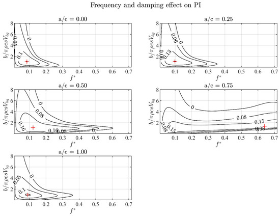
Figure 7.
Efficiency of the semi-activated flapping foil, plotted for , , and . The maximum efficiency is observed at and . Crosses refer to points of maximum efficiency.
In the case of , we observe a wider range of frequencies where is greater than zero, compared to the other cases. For this case, [39] observed a monotonic increase in performance with frequency. For this case, further investigation of this interesting behavior is required and is left as a subject for future work.
Next, the planform shape of the foil is studied. For this reason, a linear span-wise distribution of the chord is assumed, determined by the chord ration between the middle and the tip of the foil , and the foil is swept backwards by an angle , as can be seen in Figure 8.

Figure 8.
Planform of hydrofoil. The foil is swept by an angle .
The performance of foils with different planforms is shown in Figure 9. The simulations are performed for a foil with and NACA0005 cross section. The damping coefficient and the frequency are taken equal to those maximizing the performance of the rectangular foil, and . The pivot axis is located at . The range of considered is from 0.2 to 1, and ranges from 0 to 20 degrees. The special case of the rectangular foil is also considered and has and .

Figure 9.
Effect of the planform parameters on the performance of the device.
The decrease in causes the performance to decline, and the introduction of a sweep angle has a diminishing effect on the performance of the device, something to be expected, as the center of pressure moves backwards, increasing the moment generated by the hydrodynamic forces, resulting in more power being needed on average to sustain the pitch motion (see Figure 10). In the range of parameters examined, there is a region where the efficiency of the device becomes negative. This region is wider (in terms of ) for chord ratios near 1, and becomes narrower as the chord ratio decreases.

Figure 10.
Effect of the sweep angle on the center of pressure. The sweep angle moves the average center of pressure further from the leading edge (LE) ().
In Figure 11, we show the effect of placing the pivot axis of the swept foil for at the period averaged center of pressure (). In this case, the performance of the swept and non-swept foils shows only small differences for the entire range of examined. It is also interesting that the swept foil shows a significant increase in performance, while the non-swept foil suffers about a 5% decrease in performance. Higher sweep angles (e.g., ) are not shown in Figure 11, as the pivot axis would be located at , as the pivot axis would be outside the planform; the investigation of this interesting configuration, which could be implemented by using a swing arm, is left as a subject for future work.
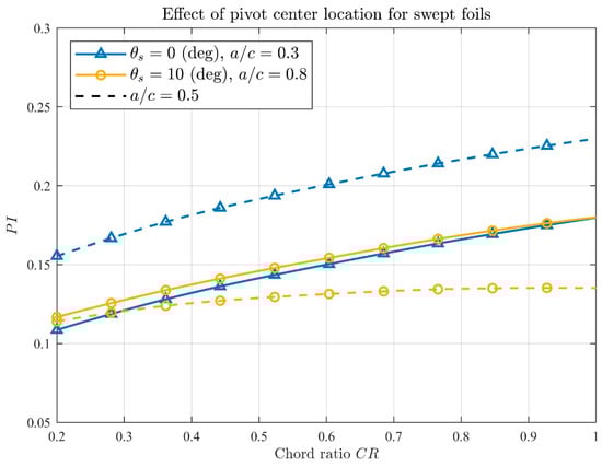
Figure 11.
Effect of the pivot axis location on the performance of the swept foil. Continuous line: , dashed line: .
Another way to counteract the drop in performance is to tilt the pivot axis backwards. For this configuration, four distinct cases are examined (see Figure 12). The cases are: (a) , , (b) , , (c) , , (d) , . The performance of the device after this correction is applied is shown in Figure 13. Rotating the foil about a tilted axis can increase the performance up to 2% for the maximum-performance frequency in case (b), but even in this case the performance of the swept-back foils cannot surpass that of the rectangular foil. Both methods examined in the present work for mitigating the negative effect of the planform shape on the performance of the oscillating-foil device do not manage to increase the performance of the swept foils significantly. However, slightly swept foils are also considered in the design stage of the studied oscillating-foil system, as they have the property to align better with changing current flow direction.
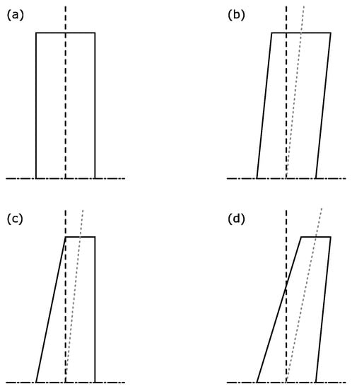
Figure 12.
The four planforms examined in the swept foil performance comparison. (a) , , (b) , , (c) , , (d) , .
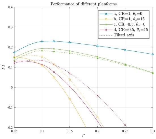
Figure 13.
Comparison of the performance for the cases (a), (b), (c) and (d). Results for both straight and tilted pivot axes are shown.
4.3. Twin-Foil Configuration
In this subsection, we study the performance of a parallel twin-foil configuration, introducing a second foil placed below the first at an initial vertical distance . This configuration has been studied for thrust production (see, e.g., [41]), and for marine energy extraction (see, e.g., [42]). In [42], the energy extraction capabilities of the device were studied by imposing predetermined pitching and heaving motions on both foils for the 2D case. The effect of elasticity was also taken into account in that work. Initially, the two foils are placed exactly above each other, moving in a symmetric way, in order to assess the effect of the vertical distance on the performance of the device. Next, a staggered configuration is studied with a horizontal distance and a phase difference between the foils, as shown in the drawing of Figure 14. In the following simulations, the spring coefficient is taken to be in order to keep the two foils oscillating about a constant vertical location.

Figure 14.
Staggered twin-foil configuration. is the vertical mean foil distance and is the horizontal foil distance.
For the case of the two foils moving symmetrically (), the performance of the device can increase significantly as the distance decreases, as illustrated in Figure 15. When this happens, the minimum distance between the foils () becomes small and the interaction effects get more pronounced. For the case of , for example, where , the performance increases by about 6% for . It should be noted that for small vertical distances and small values of frequency, the foils collide, something that should be prohibited. For this reason, for , only part of the curves are presented for higher frequencies in Figure 15.

Figure 15.
Performance of the twin-foil system for , and . The oscillation parameters are ,.
In Figure 16, the effect of the phase difference and the horizontal distance of the foils on the performance of the device is shown. The device shows maximum performance at and . This means that the “ground effect” plays a significant role in increasing the performance of the device. While higher values of the horizontal distance could be presented, the results obtained with the wake model adopted in the present work would introduce fictitious effects. For this reason, results were obtained only for values of smaller than 0.5.
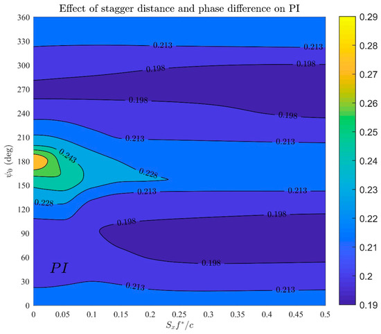
Figure 16.
Performance index of the twin-foil system for the case of . The contours show the performance index of the system for and .
4.4. Comparison with Turbines
In this subsection, we compare the performance of the devices with one, two and three foils, with a proposed tidal turbine design. For this comparison, the equivalent tip speed ratio (TSR) for the oscillating-foil devices should be defined, starting by finding the diameter of the disk with an equal area to that swept by the foils
the equivalent TSR is defined as
In Figure 17, the performance of the oscillating-foil devices studied in the previous subsections, with one, two and three foils in parallel configuration and phase difference, is compared against the experimental data for a model tidal turbine in a cavitation tank, with three blades, hub pitch angle and current velocity , referenced from [43]. The vertical foil distance here is and the springs were ignored .
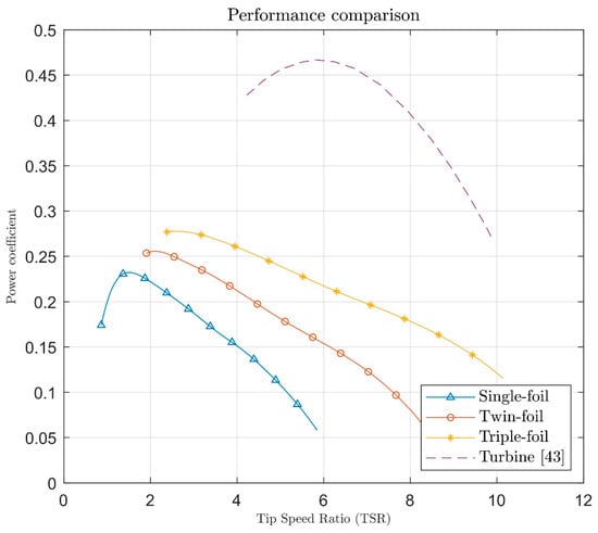
Figure 17.
Comparison of oscillating-foil device performance with that of a horizontal axis turbine. Oscillating-foil designs with up to three foils are presented, illustrating an increase in performance as the number of foils increases. The oscillating foil yields a peak efficiency at lower frequencies than the turbine.
It is apparent that by increasing the number of foils in the oscillating-foil configuration, the performance of the device increases, but still, the oscillating-foil devices studied here reach about 50% of the capability of the turbine. It should be noted here, however, that by increasing the pitch amplitude, the performance increases, reaching a maximum at 76.3 degrees [19]. These devices can also operate near the water surface to simultaneously extract energy from waves [18]. Furthermore, tandem configurations of oscillating foils can take advantage of the unsteady phenomena at the wake [26]. Considering these three practices, along with proper optimization of the device, can potentially allow oscillating-foil devices to compete with tidal turbines. It is also noteworthy that oscillating foils have peak performances at TSRs significantly lower than that of the turbine, supporting the argument that in real-world applications they will be friendlier to the marine environment near the installation.
5. Discussion
Oscillating foils are studied in this work as novel biomimetic systems for the extraction of tidal stream energy. For modeling the performance of semi-activated oscillating foil(s), a mathematical problem is formulated, describing the coupling between the hydrodynamics of the unsteady flow around the oscillating foil(s) and the dynamical system including the power take-off. The hydrodynamics are numerically treated by BEM, and the solution provides information concerning the instantaneous lift force of the foil, as well as the foil moment about the pivot axis. The lift force is then used to integrate the dynamical system in time and obtain the heaving motion of the foil, and the non-linear fluid-structure couplings are treated by an iterative scheme. In order to accelerate computations, the present BEM is implemented using GPGPU programming and object-oriented principles for extensibility. A mixed-precision scheme is used, resulting in an enhanced performance of the computational code. Fast calculation of integrals is achieved by using a fast and elegant quadrature routine for evaluating singular surface integrals.
The validity of the present method is illustrated by comparisons against experimental data. Then, the present model is used to study the operational characteristics of the device, first in the case of a single-foil system. A systematic investigation of the geometry of the foil is performed, showing that moderate values of performance index could be achieved by unswept foils. Since a leading edge sweep angle could have some beneficial effect on the alignment of the device with changing current flow direction, an investigation is performed, showing that the sweep angle reduces the performance of the device, as the center of foil pressure moves backwards, increasing the required pitching moment and reducing the net power output. To improve the performance of swept foils, the effect of placing the pivot axis closer to the pressure center is considered. In that configuration, the performance of the studied swept foil increased by 4.5%, while the performance of the non-swept foil decreased by 5%. Overall, when the pivot axis is located close to the period-averaged center of pressure, the gap between the performance of the non-swept foil and the swept foil becomes smaller, and in fact the slightly swept foil performs better but does not exceed the performance of the rectangular foil with the pivot axis located at the mid-chord (see Figure 11). Another way to counteract the drop in performance is to tilt the pivot axis backwards. In the range of the design parameters studied, rotating the foil about a tilted axis can increase the performance up to 2% for the band of frequencies near the maximum performance, but even in this case, the performance of the swept-back foils cannot surpass that of the rectangular foil. Subsequently, a twin-foil configuration is investigated for increasing the performance of the system, by utilizing the strong interaction effects between the foils. Initially, the two foils move in a symmetric way, in order to assess the effect of the vertical distance on the performance of the device. At the next step, a staggered configuration is studied with a horizontal distance and a phase difference between the foils. For the case of the two parallel foils moving symmetrically (), the performance of the device can increase significantly as the distance between them decreases. For the case of , for example, where , the performance increases by about 6% for . It should be noted that for small vertical distances and small values of frequency, the foils collide, something that should be prohibited. Even when considering the effect of the phase difference and the horizontal distance of the foils (staggered configuration), the system shows maximum performance at and (parallel configuration). This means that the “ground effect” could have a significant role in increasing the performance of the device and, for the cases studied, the optimal configuration is the parallel one.
Furthermore, the performance of multiple oscillating foils (single foil, parallel twin-foil arrangement and a system with three parallel foils) is compared to the performance of tidal turbines. It is apparent that by increasing the number of foils in the oscillating-foil configuration, the performance of the device increases. A two-foil configuration shows an 11% relative increase in performance compared to the single-foil device, and a three-foil configuration presents a 21% relative increase in performance. Still, the oscillating-foil devices studied here reach about 50% of the capability of the turbine. It should be noted here, however, that by increasing the pitch amplitude, the performance increases, reaching a maximum at 76.3 degrees [19]. These devices can also operate near the water surface to simultaneously extract energy from waves [18]. Furthermore, tandem configurations of oscillating foils can take advantage of the unsteady phenomena at the wake [26]. Considering these three practices, along with proper optimization of the device, can potentially allow oscillating-foil devices to compete with tidal turbines. It is also noteworthy that oscillating foils have peak performances at significantly lower frequencies in comparison with the turbine, supporting the argument that in real-world applications, they will be friendlier to the marine environment near the installation.
6. Conclusions
In the present work, a biomimetic semi-activated oscillating-foil device with single or multiple foils is studied for the extraction of marine renewable energy. For the present investigation, an unsteady boundary element method (BEM) is used for the simulation of 3D lifting flows coupled with the dynamics of the system including inertia, spring and damping forces, the latter used to model the power take-off. In general, it is illustrated that the present method and the computational code, after enhancement and further verification, are useful and efficient tools for the design and control of such devices for the extraction of marine renewable energy.
To summarize, the present method was used first to study the performance characteristics of the single-foil system. The effects on performance of the damping coefficient, the oscillation frequency and the locations of the pivot axis and pitching amplitude were studied, and the optimal operational parameters were determined. Also, the effect of the planform shape was considered in terms of a sweep angle and the chord ratio between the tips and the middle of the foil, and the results indicate that rectangular foils perform better. Next, the two-foil system was investigated. For this configuration, the distance between the two foils and the phase difference of the pitch motion can influence the performance significantly, and the maximum performance is achieved when the foils operate close to each other and perform symmetric pitching motions. Finally, the performance of the single, twin and triple foil systems was compared against the performance of a horizontal axis turbine system. Even though the performance of the oscillating foils does not surpass that of tidal turbines, the performances of the twin-foil and triple-foil systems are 11% and 21% higher than that of the single-foil system, respectively.
Future work includes the introduction of a non-linear model for the wake and the pressure-Kutta condition at the trailing edge of the foils, and also the inclusion of the free surface and bottom in the simulation. Moreover, hydroelastic effects can be included in the modeling as this can improve the performance of these devices further [44,45]. These will significantly increase the computational load, and thus, a modern high performance computing (HPC) code that scales well on clusters with GPUs should be developed. Also, the investigation of larger angles of attack, including viscous effects, in the modeling and experimental verification is left as a subject for future work. Finally, having established the framework of multiple-foil configurations, a more systematic investigation of the effect of the number of foils on the performance should be performed in the future.
Author Contributions
This work is based on the diploma thesis of P.E.K. supervised by K.A.B. The main draft of the text and numerical simulations were handled by P.E.K. and E.S.F. All authors agreed with the final form of this article.
Funding
This research received no external funding.
Conflicts of Interest
The authors declare no conflict of interest.
Abbreviations
| BEM | Boundary Element Method |
| GPU | Graphics Processing Unit |
| GPGPU | General Programming on Graphical Processing Unit |
| LEV | Leading Edge Vortices |
| TE | Trailing Edge |
| LE | Leading Edge |
| IBVP | Initial Boundary Value Problem |
| IVP | Initial Value Problem |
| BIE | Boundary Integral Equation |
| PTO | Power Take-Off |
Nomenclature
| Heave response | |
| Pitch angle | |
| Pitch amplitude | |
| Foil mass | |
| Damping coefficient | |
| Spring coefficient | |
| Lift force | |
| Angular frequency of pitching motion | |
| Performance index | |
| Water density | |
| Disturbance potential field | |
| Background current velocity | |
| Non-dimensional frequency | |
| Chord length | |
| Location of pivot axis from leading edge | |
| Sweep angle | |
| Chord ratio | |
| Vertical distance between two foils | |
| Horizontal distance between two foils | |
| TSR | Tip speed ratio |
References
- Khan, M.J.; Bhuyan, G.; Iqbal, M.T.; Quaicoe, J.E. Hydrokinetic energy conversion systems and assessment of horizontal and vertical axis turbines for river and tidal applications: A technology status review. Appl. Energy 2009, 86, 1823–1835. [Google Scholar] [CrossRef]
- Triantafyllou, M.S.; Triantafyllou, G.S.; Yue, D.K.P. Hydrodynamics of fishlike swimming. Annu. Rev. Fluid Mech. 2000, 32, 33–53. [Google Scholar] [CrossRef]
- Triantafyllou, M.S.; Techet, A.H.; Hover, F.S. Review of experimental work in biomimetic foils. IEEE J. Ocean. Eng. 2004, 29, 585–594. [Google Scholar] [CrossRef]
- Politis, G.K.; Tsarsitalidis, V.T. Flapping wing propulsor design: An approach based on systematic 3D-BEM simulations. Ocean Eng. 2014, 84, 98–123. [Google Scholar] [CrossRef]
- Rozhdestvensky, K.V.; Ryzhov, V.A. Aerohydrodynamics of flapping-wing propulsors. Prog. Aerosp. Sci. 2003, 39, 585–633. [Google Scholar] [CrossRef]
- Bowker, J.A. Coupled Dynamics of a Flapping Foil Wave Powered Vessel. Ph.D. Thesis, University of Southampton, Southampton, UK, 2018. [Google Scholar]
- Filippas, E.S. Hydrodynamic Analysis of Ship and Marine Biomimetic Systems in Waves Using GPGPU Programming. Ph.D. Thesis, National Technical University of Athens, Athens, Greece, 2019. [Google Scholar]
- Filippas, E.S.; Belibassakis, K.A. Hydrodynamic analysis of flapping-foil thrusters operating beneath the free surface and in waves. Eng. Anal. Bound. Elem. 2014, 41, 47–59. [Google Scholar] [CrossRef]
- Belibassakis, K.A.; Filippas, E.S. Ship propulsion in waves by actively controlled flapping foils. Appl. Ocean Res. 2015, 52, 1–11. [Google Scholar] [CrossRef]
- Filippas, E.S. Augmenting Ship Propulsion in Waves Using Flapping Foils Initially Designed for Roll Stabilization. Procedia Comput. Sci. 2015, 66, 103–111. [Google Scholar] [CrossRef]
- Bøckmann, E. Wave Propulsion of Ships. Ph.D. Thesis, Norwegian University of Science and Technology, Trondheim, Norway, 2015. [Google Scholar]
- Bøckmann, E.; Steen, S. Model test and simulation of a ship with wavefoils. Appl. Ocean Res. 2016, 57, 8–18. [Google Scholar] [CrossRef]
- Bøckmann, E.; Yrke, A.; Steen, S. Fuel savings for a general cargo ship employing retractable bow foils. Appl. Ocean Res. 2018, 76, 1–10. [Google Scholar] [CrossRef]
- BIO-PROPSHIP: Augmenting Ship Propulsion in Rough Sea by Biomimetic-Wing System. 2007–2013. Available online: http://arion.naval.ntua.gr/~biopropship/index_en.html (accessed on 20 November 2019).
- McKinney, W.; DeLaurier, J. Wingmill: An oscillating-wing windmill. J. Energy 1981, 5, 109–115. [Google Scholar] [CrossRef]
- DeLaurier, J.D.; Harris, J.M. Experimental study of oscillating-wing. J. Aircr. 1982, 19, 368–373. [Google Scholar] [CrossRef]
- Xiao, Q.; Zhu, Q. A review on flow energy harvesters based onflapping foils. J. Fluids Struct. 2014, 46, 174–191. [Google Scholar] [CrossRef]
- Filippas, E.S.; Gerostathis, T.P.; Belibassakis, K.A. Semi-activated oscillating hydrofoil as a nearshore biomimetic energy system in waves and currents. Ocean Eng. 2018, 154, 396–415. [Google Scholar] [CrossRef]
- Kinsey, T.; Dumas, G. Parametric study of an oscillating airfoil in a power-extraction regime. AIAA J. 2008, 46, 1318–1330. [Google Scholar] [CrossRef]
- Huxham, G.H.; Cochard, S.; Patterson, J. Experimental parametric investigation of an oscillating hydrofoil tidal stream energy converter. In Proceedings of the 18th Australasian Fluid Mechanics Conference (AFMC), Launceston, Australia, 3–7 December 2012. [Google Scholar]
- Zhu, Q. Optimal frequency for flow energy harvesting of a flapping foil. J. Fluid Mech. 2011, 675, 495–517. [Google Scholar] [CrossRef]
- Betz, A. Das maximum der theoretisch möglichen ausnutzung des windes durch windmotoren. Z. Gesamte Turbinenwesen 1920, 20, 26. [Google Scholar]
- Dabiri, J.O. Renewable fluid dynamic energy derived from aquatic animal locomotion. Bioinspir. Biomim. 2007, 2, L1–L3. [Google Scholar] [CrossRef]
- Young, J.; Lai, J.C.; Platzer, M.F. A review of progress and challenges in flapping foil power generation. Prog. Aerosp. Sci. 2014, 67, 2–28. [Google Scholar] [CrossRef]
- Zhu, Q.; Zhangli, P. Mode coupling and flow energy harvesting by a flapping foil. Phys. Fluids 2009, 21, 033601. [Google Scholar] [CrossRef]
- Kinsey, T.; Dumas, G. Optimal tandem configuration for oscillating foils hydrokinetic turbine. J. Fluids Eng. 2012, 134, 031103. [Google Scholar] [CrossRef]
- Karbasian, H.R.; Esfahani, J.A.; Barati, E. Simulation of power extraction from tidal currents by flapping foil hydrokinetic turbines in tandem formation. Renew. Energy 2015, 81, 816–824. [Google Scholar] [CrossRef]
- Isogai, K.; Abiru, H. Study of Multi-Wing Configurations of Elastically Supported Flapping Wing Power Generator. Trans. Jpn. Soc. Aeronaut. Space Sci. 2012, 55, 133–142. [Google Scholar] [CrossRef]
- Isogai, K.; Abiru, H. Lifting-Surface Theory for Multi-Wing Configurations of Elastically Supported Flapping Wing Power Generator. Trans. Jpn. Soc. Aeronaut. Space Sci. 2012, 55, 157–165. [Google Scholar] [CrossRef][Green Version]
- Politis, G.K. Unsteady wake rollup modeling using a molifier based filtering technique. Dev. Appl. Ocean Eng. 2016, 5, 1–28. [Google Scholar] [CrossRef]
- Politis, G.K. Application of a BEM time stepping algorithm in understanding complex unsteady propulsion hydrodynamic phenomena. Ocean Eng. 2011, 38, 699–711. [Google Scholar] [CrossRef]
- Lyness, J.N. Notes on the adaptive simpson quadrature routine. J. ACM 1969, 16, 483–495. [Google Scholar] [CrossRef]
- Gander, W.; Gautschi, W. Adaptive quadrature—Revisited. BIT Numer. Math. 2000, 40, 84–101. [Google Scholar] [CrossRef]
- Abramowitz, M.; Stegun, I.A.; Morse, P.M. Handbook of Mathematical Functions: With Formulas, Graphs, and Mathematical Tables; Applied Mathematics Series 55; Courier Corporation: New York, NY, USA, 1965. [Google Scholar]
- Michels, H.H. Abscissas and weight coefficients for lobatto quadrature. Math. Comput. 1963, 17, 237–244. [Google Scholar] [CrossRef]
- Richardson, L.F.; Arthur, J.G. Viii. The deferred approach to the limit. Philos. Trans. R. Soc. Lond. Ser. A Math. Phys. Eng. Sci. 1927, 226, 299–361. [Google Scholar] [CrossRef]
- Trompoukis, X.S. Solving Aerodynamic-Aeroelastic Problems on Graphics Processing Units. Ph.D. Thesis, School of Mechanical Engineering, National Technical University of Athens, Athens, Greece, 2012. [Google Scholar]
- Nishimura, N. Fast multipole accelerated boundary integral equation. Appl. Mech. Rev. 2002, 55, 299–324. [Google Scholar] [CrossRef]
- Zhu, Q.; Haase, M.; Wu, H.C. Modeling the capacity of a novel flow-energy harvester. Appl. Math. Model. 2009, 33, 2207–2217. [Google Scholar] [CrossRef]
- Papadakis, G.; Filippas, E.S.; Douras, D.; Belibassakis, K.A. Effects of viscosity and nonlinearity on 3D flapping-foil thruster for marine applications. In Proceedings of the OCEANS, Marseille, France, 17–20 June 2019. [Google Scholar]
- Politis, G.; Tsarsitalidis, V. Biomimetic propulsion using twin oscillating wings. In Proceedings of the Third International Symposium on Marine Propulsors (SMP’13), Launceston, Tasmania, Australia, 5–7 May 2013. [Google Scholar]
- Liu, W.; Xiao, Q.; Cheng, F. A bio-inspired study on tidal energy extraction with flexible flapping wings. Bioinspir. Biomim. 2013, 8, 036011. [Google Scholar] [CrossRef] [PubMed]
- Bahaj, A.S.; Molland, A.F.; Chaplin, J.R.; Batten, W.M.J. Power and thrust measurements of marine current turbines under various hydrodynamic flow conditions in a cavitation tunnel and a towing tank. Renew. Energy 2007, 32, 407–426. [Google Scholar] [CrossRef]
- Priovolos, A.K.; Filippas, E.S.; Belibassakis, K.A. A vortex-based method for improved flexible flapping-foil thruster performance. Eng. Anal. Bound. Elem. 2018, 95, 69–84. [Google Scholar] [CrossRef]
- Anevlavi, D.E.; Filippas, E.S.; Karperaki, A.E.; Belibassakis, K.A. Hydroelastic modelling of flapping foils operating as flow and wave energy devices. In Proceedings of the European Wave and Tidal Energy Conference Series, Napoli, Italy, 1–6 September 2019. [Google Scholar]
© 2019 by the authors. Licensee MDPI, Basel, Switzerland. This article is an open access article distributed under the terms and conditions of the Creative Commons Attribution (CC BY) license (http://creativecommons.org/licenses/by/4.0/).