Identification of Crack Length and Angle at the Center Weld Seam of Offshore Platforms Using a Neural Network Approach

Abstract

The reconstruction algorithm for the probabilistic inspection of damage (RAPID) is aimed at localizing structural damage via the signal difference coefficient (SDC) between the signals of the present and reference conditions. However, tomography is only capable of presenting the approximate location and not the length and angle of defects. Therefore, a new quantitative evaluation method called the multiple back propagation neural network (Multi-BPNN) is proposed in this work. The Multi-BPNN employs SDC values as input variables and outputs the predicted length and angle, with each output node depending on an individual hidden layer. The cracks of different lengths and angles at the center weld seam of offshore platforms are simulated numerically. The SDC values of the simulations and experiments were normalized for each sample to eliminate external interference in the experiments. Then, the normalized simulation data were employed to train the proposed neural network. The results of the simulations and experimental verification indicated that the Multi-BPNN can effectively predict crack length and angle, and has better stability and generalization capacity than the multi-input to multi-output back propagation neural network.

1. Introduction

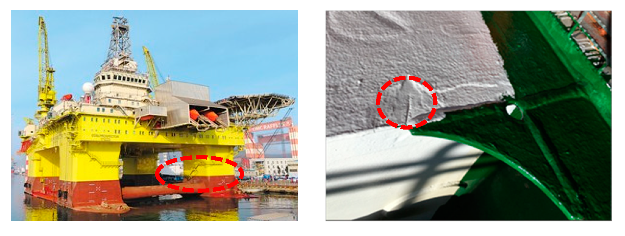
In recent years, efforts have been increasingly focused on the structural health monitoring (SHM) of offshore platforms for the purpose of structural safety, and crack detection at the center weld seams of platforms is one of the hot spots. Influenced by various environmental factors, the crack is shown in Figure 1. The Lamb wave technique shows great promise because of its excellent propagation capability and high sensitivity to changes in structural properties [1,2].

Lamb wave tomography originates from computed tomography in clinical applications, and it has been widely investigated in recent decades. Amplitude attenuation and time of flight are the most commonly used tomography features. On the basis of these features, filtered back projection and the algebraic reconstruction technique are proposed [3,4]. However, determining precisely the ToF or amplitude of scattered signals is difficult, and this drawback limits the application of these methods [5].

The signal difference coefficient (SDC) based on the probabilistic reconstruction algorithm has been widely used, mainly because it can detect small defects with a sparse sensor network [6,7]. Therefore, this method has attracted much attention.

Hay [8] proposed the well-known reconstruction algorithm for the probabilistic inspection of damage (RAPID), which detects defects by calculating the differences in the Lamb wave signals between intact and faulty conditions. Ye introduced virtual sensing paths to reduce blind zones and proposed digital damage fingerprints to highlight the changes in signals corresponding to the presence of damage [9,10,11]. In sensor detection, Mehdi Foumani, Kate Smith-Miles and Indra Gunawan proposed a heuristic method to study the inspection integration framework, in order to minimize the automatic inspection system [12,13,14], it can also be applied to marine science and engineering. Marco Ulricha and Gregor Lux proposed an adapted probabilistic roadmap method to search for valid paths between the measurement poses [15]. Lin proposed the local SDC, which significantly improves the resolution of localization images [16,17]. Moreover, they analyzed the influences of data length on the SDC and tomogram [18]. Mu proposed a localisation approach for marine platform damage based on particle swarm optimisation (PSO). This method reduces the positioning time obviously and ensures the high positioning accuracy [19]. It also improves the real-time performance of offshore platform monitoring [20]. They also proposed for the first time to locate the crack tip by diffraction wave, which provides a better method for the analysis of crack length and angle [21]. Thus far, most research focuses on the localization of through-thickness holes. However, in reality, the shape of defects rarely resembles a hole. At the same time, the shape of defects can affect the received signals significantly, and adversely influence the SDC. As a result, an intelligent algorithm should be established for the quantitative analysis of cracks.

Artificial neural networks are effective alternatives in solving inverse problems, owing to their strong nonlinear mapping ability, error tolerance, and self-learning capability [22]. In theory, a back propagation (BP) neural network with a single hidden layer can approximate any nonlinear mapping, provided that the sample is sufficient and that the parameter settings of the network are reasonable [23]. The progress in neural networks has greatly stimulated research. Studies [24] have reported the automatic classification systems of defects, elimination of the adverse effects of environmental parameters in capacitive pressure sensors [25], and pattern recognition for pipeline leakage localization systems [26]. Neural networks trained by certain samples can process enormous amounts of data and recognize the patterns of test samples in a short period. Given the nonlinear nature of the parameters involved in ultrasonic guided wave, conventional methods are prone to unreliable predictions [27]. Thus, neural networks need to be employed to predict the parameters of defects quantitatively.

The multiple back propagation neural network (Multi-BPNN) model was first proposed to detect slender cracks in weld seams of platforms, determine crack position, and achieve an accurate prediction of crack length and tilt angle. The rest of this article is organized as follows: After the introduction, a brief review of RAPID is presented. Then, the simulation model and the tomography of cracks of different lengths and angles are discussed. Next, using the crack data from RAPID as data input, the Multi-BPNN method is proposed, and the procedure of parameter determination is presented. In the next section “Performance of the Multi-BPNN,” the accuracy and generalization capacity of the proposed method are estimated, and its comparison with the multi-input to multi-output back propagation neural network (MIMO-BPNN) is detailed. An experimental verification is then carried out. Finally, several conclusions are given.

2. Review of RAPID

In RAPID, the assumption is that the probability of defect occurrence at a specific point can be estimated from the extent of signal changes in different sensor pairs resulting from this defect and its position relative to the sensor pairs [28]. But the quantitative analysis ability of this method is not high.

The SDC is a correlation analysis-based statistical index, which measures the differences between the signals of the present condition and the reference condition. That is, the difference caused by structural modification is considerable when the scale of the defect is large. Thus, the SDC plays a significant role in calculating the probability of the presence of damage. $I\left(t\right)$ and $F\left(t\right)$ denote the intact and fault signals, respectively. The SDC is defined as [29]:

$$SDC=1-\frac{Cov\left(I,F\right)}{{\sigma }_I{\sigma }_F}$$

(1)

where the covariance, is:

$$Cov\left(I,F\right)={{\displaystyle \sum }}_{k=1}^K\left(I_k-{\mu }_I\right)\left(F_k-{\mu }_F\right)$$

(2)

and

$${\sigma }_I{\sigma }_F=\sqrt{{{\displaystyle \sum }}_{k=1}^K{\left(I_k-{\mu }_I\right)}^2}\sqrt{{{\displaystyle \sum }}_{k=1}^K{\left(F_k-{\mu }_F\right)}^2}$$

(3)

In the above formula,${\mu }_I,{\mu }_F$ and ${\sigma }_I{\sigma }_F$ represent the expected values and standard deviations of the intact and faulty signals, respectively.

In RAPID, for a specific transmitter–receiver pair (Figure 2), the spatial distribution of the defect acts as a weighted matrix in a linearly decreasing elliptical pattern where the two foci of the ellipse are the two transducer locations.

$$w_{ij}\left(x,y\right)=\left[\frac{\beta -R_{ij}\left(x,y\right)}{\beta -1}\right]$$

(4)

In the above formula, $w_{ij}\left(x,y\right)$ is the weight of the input element. Here, the relative distance is:

$$R_{ij}\left(x,y\right)=\frac{\sqrt{{\left(x_i-x\right)}^2+{\left(y_i-y\right)}^2}+\sqrt{{\left(x_j-x\right)}^2+{\left(y_j-y\right)}^2}}{\sqrt{{\left(x_i-x_j\right)}^2+{\left(y_i-y_j\right)}^2}}$$

(5)

where $\left(x,y\right)$ is the coordinate of the point under estimation, $\left(X_i,Y_i\right)$ and $\left(X_j,Y_j\right)$ denote the coordinates of the $i$-th and $j$-th sensors, which act as the actuator and receiver, respectively. $\beta$ represents the scaling parameter that controls the size of the elliptical area. According to the method mentioned by Hua 16, it is determined that $\beta$ is 1.05. A large $\beta$ equates to a large elliptical detection area. As a result, the overlapped regions enlarge and, thereby, decline the localization resolution. The weighted matrix is redefined by:

$$w_{ij}\left(x,y\right)=\{\begin{array}{c}\left(\beta -R_{ij}\left(x,y\right)\right)/\left(\beta -1\right)when{R}_{ij}\left(x,y\right)<\beta \\ 0when{R}_{ij}\left(x,y\right)\ge \beta \end{array}$$

(6)

If $P_{ij}\left(x,y\right)$ denotes the probability of defect occurrence at a point from the transmitter $i$ and receiver $j$ sensor pair, the defect distribution probability within the sensor network can be expressed as a linear summation of all the signal change effects of every possible transmitter–receiver pair.

$$\mathrm{P}\left(\mathrm{x},\mathrm{y}\right)={{\displaystyle \sum }}_{i=1}^{N-1}{{\displaystyle \sum }}_{j=i+1}^N{P}_{ij}\left(x,y\right)={{\displaystyle \sum }}_{i=1}^{N-1}{{\displaystyle \sum }}_{j=i+1}^N{w}_{ij}\left(x,y\right)S_{ij}$$

(7)

where $S_{ij}$ represents the SDC of the transmitter $i$ and receiver $j$ sensor pair.

3. Performance Analysis

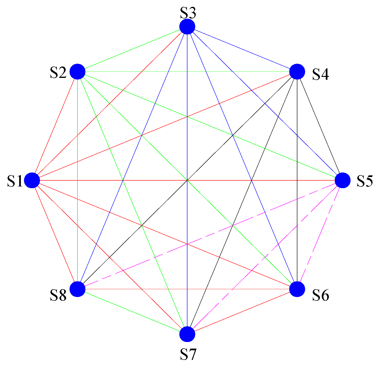
Simulation studies were carried out with ABAQUS CAETM (Dassault SIMULIA Company, Providence, Rhodes Island, USA). In the simulation model with dimensions of 760 mm (length) × 760 mm (width) × 2 mm (thickness), Q235 steel, which is commonly used in offshore platforms, was set as the material parameter. A circular sensor array, which consists of eight sensors, was arranged on the surface of the model. In this study, a five-period cycle-windowed sinusoidal tone burst signal, centered at 150 kHz, was generated as the input signal to drive the actuators. With this excitation signal, only fundamental modes A0 and S0 propagate in the model, and the wavelengths of the A0 and S0 mode waves were 26 and 18 mm, respectively. For the data acquisition process, each sensor served as an actuator while the rest served as receivers. The sensor array provided 28 sensing paths, as illustrated in Figure 3. These signals were called reference signals under intact conditions.

Several damage conditions were also simulated with the same parameters, but the simulation model contained a through-thickness rectangle crack measuring 1 mm (width) × 2 mm (thickness). The 24 simulation models used in this work varied, and their cracks showed different lengths or angles. The lengths of these cracks were 10, 20, 30 and 40 mm, and each kind of crack with the same length contained six angles, as shown in

Table 1. Crack parameters values.

Angle	Length
0°	10 mm. 20 mm. 30 mm. 40 mm.
11.25°	10 mm. 20 mm. 30 mm. 40 mm.
22.5°	10 mm. 20 mm. 30 mm. 40 mm.
30°	10 mm. 20 mm. 30 mm. 40 mm.
45°	10 mm. 20 mm. 30 mm. 40 mm.
56.25°	10 mm. 20 mm. 30 mm. 40 mm.
67.5°	10 mm. 20 mm. 30 mm. 40 mm.
75°	10 mm. 20 mm. 30 mm. 40 mm.

. The same sensor array and input signal used in the previous section were used to monitor the simulation model. These signals were called present signals under damage conditions.

Figure 4 illustrates a crack of 10 mm and 0°. The attitude angle is defined as the angle between the crack and the vertical axis. The positive angle increases when the crack rotates counterclockwise.

Unlike the crack of 0°, a tilted crack is difficult to create in the simulation model. Moreover, a tilted crack leads to irregular mesh elements, which would affect analysis accuracy. In the infinite plate, the same result is obtained by keeping the relative position between the crack and the sensor network unchanged. Therefore, a simulation model with a crack of 11.25° (Figure 5) was equivalent to the alternative model in which the sensor network rotated 11.25° clockwise. The crack after rotation remained perpendicular to the horizontal plane, and this condition helped avoid irregular meshes in the simulation model. The other four models were conducted in the same way but with inclinations of 22.5° and 56.25° (Figure 6).

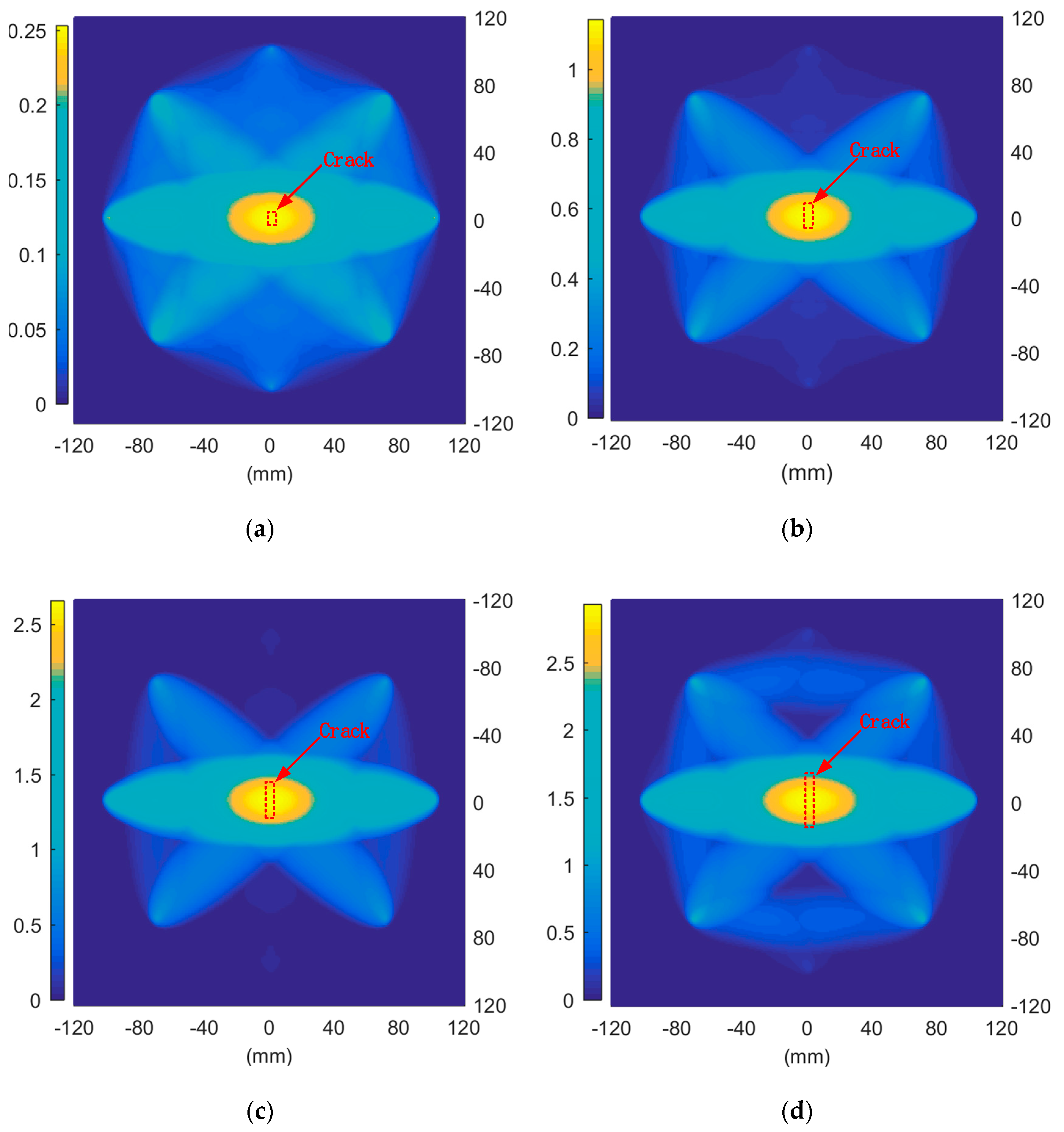
The RAPID algorithm was employed to obtain the corresponding tomograms (Figure 7 and Figure 8). The reconstruction images were divided into two regions, namely, the damage region and the background. The damage region consisted of pixels with larger probability values than the specified threshold. The damage region performed well in defect detection and localization, but the quantitative information could not be obtained for the tomograms (Figure 7 and Figure 8).

The probability values increased as the defect length expanded (Figure 7). This result indicated that a large crack exerts greater influence on the SDC. Furthermore, a large crack means that many detection areas are covered. As a result, the summation of the probability values is large. Despite the approximately linear relationship between the probability and the crack length, determining the accurate length of the crack by the linear relationship alone is difficult, because the attitude angle of the crack affects the probability values simultaneously.

Defects affect the SDC mainly because of the reflection, diffraction, and transmission of guided waves. In Figure 8, the red dotted box represents the inclination angle of the crack. The RAPID algorithm can roughly determine the inclination direction of the crack, but it cannot carry out a quantitative analysis of the inclination angle of the crack. Therefore, it is urgent to establish a model to determine the length and angle of the crack accurately. Using the SDC values of cracks obtained by RAPID, the following BPNN model can realize the quantitative analysis of cracks.

4. The Multi-BPNN Model

The conventional structure of the MIMO-BPNN (Figure 9) includes an input layer, a hidden layer, and an output layer. The MIMO network can solve coupling problems, and thus, changes in a single input variable will cause changes to the output variable simultaneously. A crack mainly influences the SDC values of some sensor paths in which the crack is located, and has a negligible impact on others. Hence, these variations in SDC values may be caused by variations in the crack length or angle. Therefore, the coupling relationship between length and angle is weak. In the following part, the Multi-BPNN is proposed to identify crack parameters instead of the MIMO-BPNN. The Multi-BPNN is a combination of several BPNNs. Each network comprises a hidden layer and an output layer. However, in the prediction model of crack length and angle, different hidden layers are used to optimize the number of nodes in the hidden layer, which is the biggest difference between Multi-BPNN and MIMO-BPNN.

The training process of the Multi-BPNN in this work involves the following steps:

(1) Network model parameters

The input layer has 28 nodes, and the corresponding input variables are SDC values of each sensing path. The outputs of the BP neural network are the predicted length and angle. From the empirical formula, the most appropriate number of hidden layer nodes is calculated as:

$$n=\sqrt{m+l}+a,a\in \left(0,10\right)$$

(8)

where $n$ is the number of hidden layer nodes, $m$ is the number of input layer nodes, $l$ is the number of output layer nodes, and $a$ is one constant between 1 and 10.

In addition, combined with a large number of experimental verification in the prediction model of crack length, the number of hidden layer nodes is set to 16, and the network of 28-16-1 type is created. In the prediction model of crack angle, the number of hidden layer nodes is set to 14, and the network of 28-14-1 type is created.

(2) Network initialization

In building a BP model, the activation functions in the hidden layer and output layer need to be selected first. Researchers generally prefer the log-sigmoid function (Logsig) due to its nonlinearity, differentiability, and monotonicity that meet the basic requirements of BP models [30]. The expression of the Logsig function is:

$$f\left(x\right)=\frac{1}{1+e^{-x}}$$

(9)

The mathematical model of the hidden layer can be described as follows:

$$H_j=f\left({{\displaystyle \sum }}_{i=1}^m{\omega }_{ji}{X}_i-{\mu }_j\right)$$

(10)

where $i$ is the number of input layers, $j$ is the number of hidden layers, ${\omega }_{ji}$ is the weighting coefficient, $X_i$ is the input variable, and ${\mu }_j$ is the threshold value of the hidden layer.

For a similar architecture, the mathematical model of the output layer is:

$$Z_k=f\left({{\displaystyle \sum }}_{j=1}^{16}{\alpha }_{kj}{H}_j-{\vartheta }_k\right)$$

(11)

where ${\alpha }_{kj}$ is the weighting coefficient, ${\vartheta }_k$ is the threshold value of the output layer, and $H_j$ is the output of the hidden layer.

(3) Parameter calculation of neural network

The initialized weights (${\omega }_{ji}$ and ${\alpha }_{kj}$) are set to random values between 0 and 1. The initialized thresholds of the hidden layers and output layers are fixed to random values between −1 and +1. The weights and threshold are updated using the BP algorithm.

The goal of the training process is to reduce the error between the predicted value and the target value. The mean-squared error (MSE) function is used to represent the accuracy of the trained neural network. The mean square error $E$ of the output variable and the target output variable in the neural network is:

$$E={{\displaystyle \sum }}_{k=1}^K\frac{1}{\mathrm{K}}{\left(z_k-Q_k\right)}^2$$

(12)

To gradually reduce $E$ over an iteration, we employ the gradient descent method to calculate the changes in weight variables. Then, the weight values are updated by back propagation.

(4) Implementation of training network

In this modeling, the data contain 32 data sets, each of which consists of 28 SDC values. The maximum network training time is set to 5000, the learning rate is set to 0.035, and the target error is $1\times {10}^{-10}$.

(5) Normalization processing

The conventional normalization process of the neural network is capable of eliminating the influence of feature dimensions. However, the SDC values of 28 paths vary with the different crack lengths and angles. The path in which the defect is localized provides the maximum SDC value. Hence, all paths are under the same dimension. Thus, the sample data of the input data set are normalized to the range of [−1, +1] in this study. Different from the processing of input data, the processing of the output data of the crack lengths and angles involves normalization.

After normalization, the normal distributed noises are added to the normalized data sets. This technique, called noise injection, is widely used to avoid over-fitting in the network [31]. Figure 10 shows that the MSE tends to be stable after 2000 training iterations and gradually converges to zero. A small MSE equates to a close distance between the output value of the BP model and the sample value. Then, the same data sets are used to test the trained network model. Thus, the parameters and structure of the neural network are reasonably suitable for crack evaluation.

5. Performance of the Multi-BPNN

The BPNN is designed to predict any crack occurrence in practice rather than in original samples. Thus, its stability and generalization need to be estimated when an unknown crack sample is tested. The stability of the network represents the capacity of the predicted value of a certain test sample to remain consistent every time. The generalization of the network refers to the capacity to predict potential crack signals, even signals with noises.

The commonly used estimation methods are random resampling, cross validation, leave-one-out, and bootstrap 21. The leave-one-out method involves taking one sample as the test data and the rest as the training data. Therefore, the maximum number of training samples is employed to train the network each time. Furthermore, the estimation results are stable and consistent.

For validating stability and general performance, leave-one-out estimations are carried out 20 times, and each sample is left out once so that the distribution range of the predicted values can be taken as the stability measurement of the network for a particular sample. When each of the 32 samples is estimated, the distribution of all the predicted values indicates the general ability of the network toward all potential cracks.

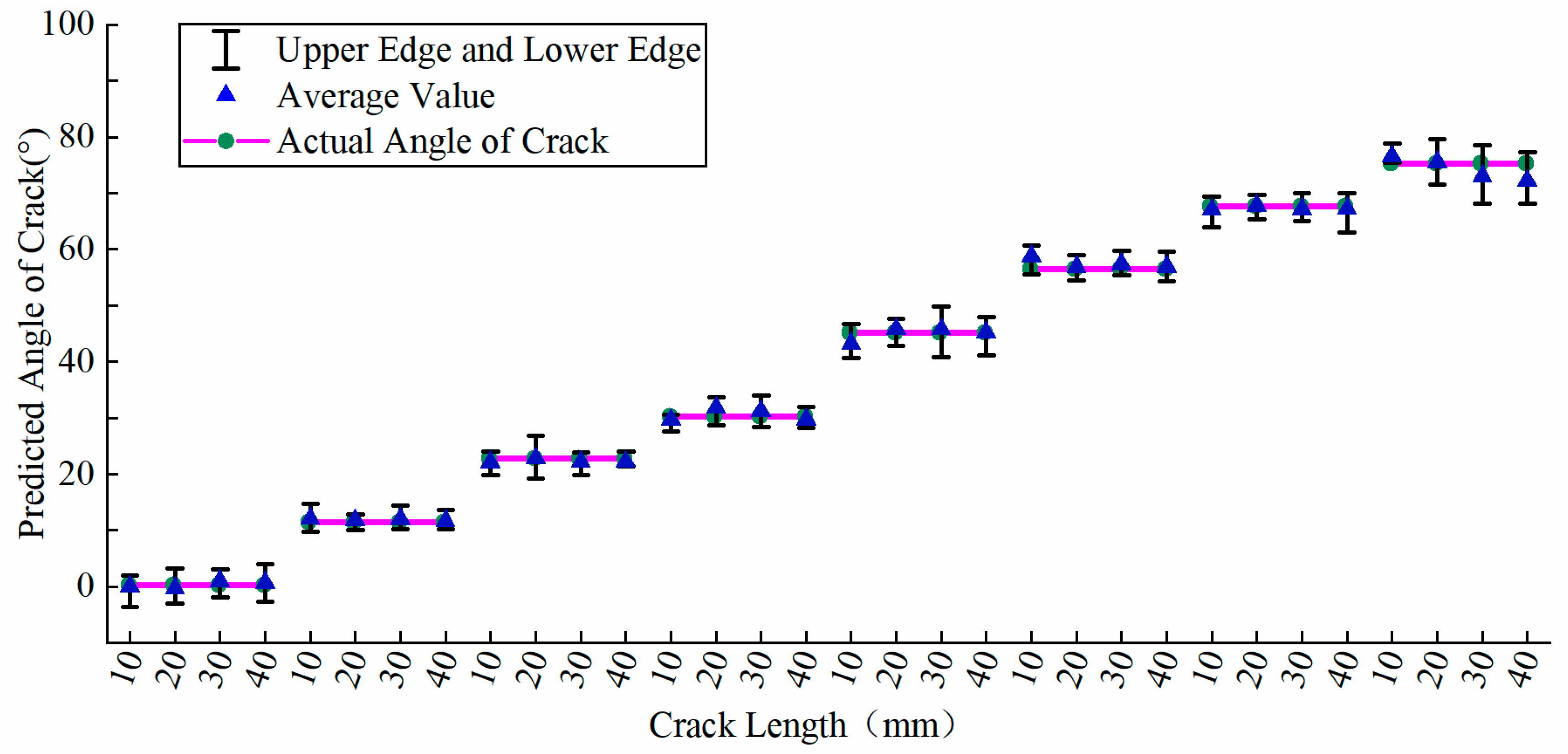
The deviation of the predicted length from the actual values varies greatly from a certain length to another. Figure 11 clearly shows that the proposed network is capable of predicting 10 mm-long cracks with considerable accuracy. With an increase in crack length, the law of ultrasonic propagation becomes increasingly complicated. When the crack is close to or larger than the wavelength, the phenomenon of reflection and diffraction occur at the crack. As a result, the sensing paths in which the crack is located are influenced due to diffraction. The sensing paths in which the crack is not located may be affected by the reflection wave. Therefore, the SDC values are highly complex when the length is 20, 30, or 40 mm in this study. Inevitably, the predicted result is not as stable and accurate as that for the case of the 10 mm length, as shown in Figure 11.

Different from the predicted length values, the predicted angles indicate considerable stability and accuracy. As mentioned above, when the crack length remains unchanged, the capacity of reflection and diffraction remains the same. For a crack located at the center of the sensor array, a change in crack angle causes a deviation in incidence angle, and all sensing paths become affected by the same propagation laws. Therefore, the proposed network performs well in predicted angles, as shown in Figure 12.

Although the generalization ability of the proposed network fluctuates, it is apparently better than the MIMO-BPNN. Each predicted value fluctuates violently in Figure 13 and Figure 14.

As mentioned by Mehdi Foumani and Kate Smith-Miles [13], in all data results, if the sample data that should be accepted is rejected, it is a type I error; if the sample data that should be rejected is accepted, it is a type II error. In order to improve the accuracy of the results, we should adopt multi-test accepts policy, and take the mean value of the calculation results.

Table 2. Predicted deviation range of the mean.

Predicted Parameter	Multi-BPNN	MIMO-BPNN
10 mm	−2.5%~+15.9%	−19.3%~+57.2%
20 mm	−3.2%~+5.5%	−34.8%~+27.2%
30 mm	+2.0%~+9.3%	−19.8%~+29.9%
40 mm	+1.1%~+6.0%	−21.1%~+24.3%
0°	−0.3~+0.93	−0.006~+0.6
11.25°	−3.6%~+7.3%	−4.4%~+13.8%
22.5°	−2.0%~+1.3%	−2.0%~+15.7%
30°	−1.3%~+5.8%	−7.6%~+7.6%
45°	−4.0%~+1.7%	−10.4%~+2%
56.25°	−1.0%~+4.3%	−0.2%~+14.6%
67.5°	−0.7%~+0.4%	−5.0%~+2.0%
75°	−3.8%~+1.9%	−2.0%~+6.5%

shows the upper and lower limits of the deviation rate of the predicted sample mean values in the Multi-BPNN and MIMO-BPNN, where the zero-degree angle cannot calculate the deviation rate. The table clearly shows that the stability and accuracy of the Multi-BPNN mode are significantly better than those of MIMO-BPNN.

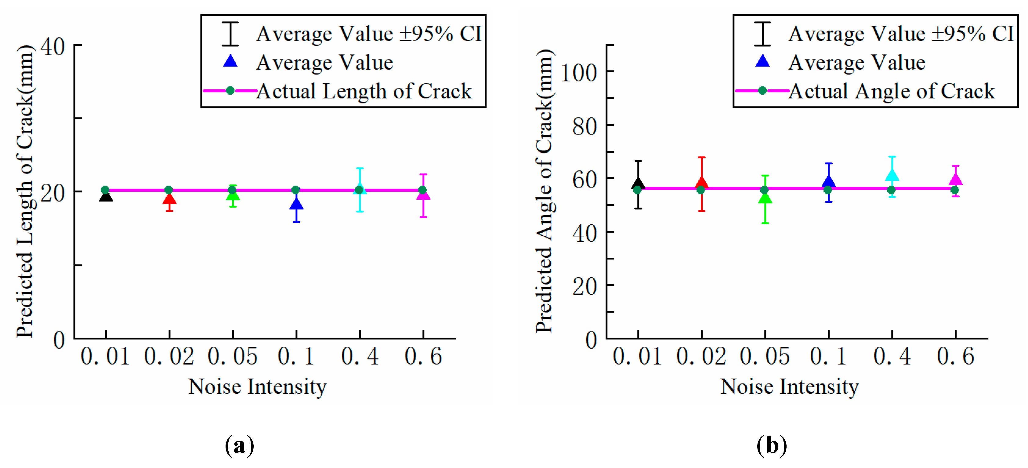
To verify the anti-interference performance of the Multi-BPNN, we added noise signals of different intensities to the data of each test crack before they were normalized. The crack with a dip angle of 22.5° and a length of 20 mm was used to predict its length, and the crack with a dip angle of 56.25° and a length of 40 mm was used to predict its angle. The results are shown in Figure 15. After the addition of noise interference of different intensities, the predicted mean values of crack length and angle appear to be close to the real values.

6. Experimental Verification

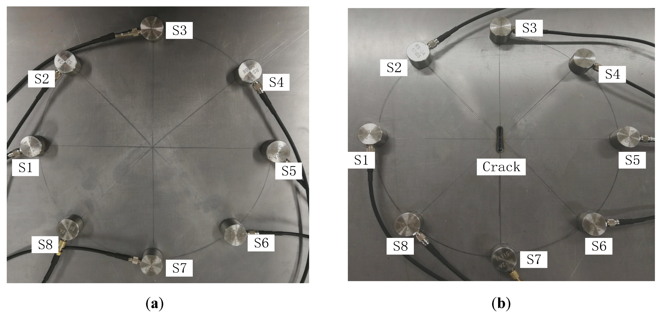
In the actual detection process of plate cracks, noise interference, temperature, humidity, and other influencing factors may be noted. To verify the feasibility of the method, we carried out an experiment. The schematic of the sensor arrangement in the healthy state and the current state is shown in Figure 16. The crack has a length of 20 mm and tilt angle of 0°. The center of the circle is the coordinate origin, and eight sensors are evenly arranged on the circumference.

Figure 17 is a schematic of the experimental device. The DS2-8B signal acquisition instrument (RIGOL, Suzhou, China) uses a frequency of up to 2.5 MHz and can realize eight channels of synchronous acquisition. The Smart AE model amplifier has a gain of 40 dB and signal bandwidth of 20 kHz–1500 kHz. The FG1022 signal generator (UNI-T, Guangzhou, China) has a sampling rate of 125 MS/s and two arbitrary waveform generation channels. The RS-2A sensor center frequency is 150 kHz, and the frequency range is 50–400 kHz. The plate used in the experiment is a Q235 steel plate of 1 m, the Poisson’s ratio is 0.3, and the elastic modulus is $2\times {10}^{11}$ Pa.

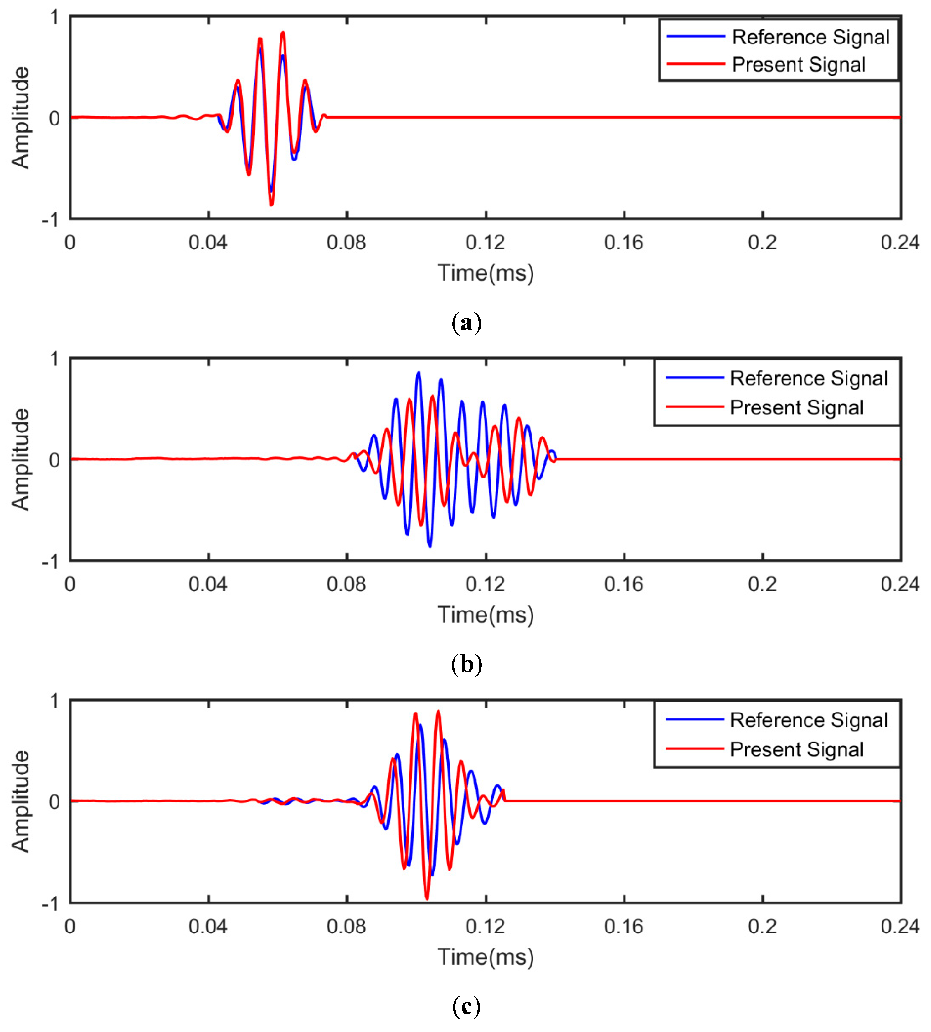
Using the DS2-8B signal acquisition instrument, the signals of seven receivers from S2 to S8 are collected when the S1 transmitter is stimulated. By analogy, the transmitters up to the S7 transmitter are excited while the S8 receiver receives the signal. The waveform data of each transmitter–receiver pair in the healthy state and current state are obtained with the fixed sensor unchanged. Figure 18 shows the comparison of the reference signal with the present signal at S1 excitation–S2 receiver, S1 excitation–S5 receiver, and S2 excitation–S6 receiver. Although no cracks are observed in the S1–S2 path, the present signal is slightly different from the reference signal, due to external interference factors, such as temperature, sensor inconsistency, and coupling inconsistency. Different from the S1–S2 path, the S1–S5 path presents obvious crack. Similar to that in the S1–S5 path, the difference between the present signal and the reference signal in the S2–S6 path is also apparent. However, such difference is greater in the S1–S5 path than in the S2–S6 path because the length of the crack projected in the vertical direction of the S1–S5 path is longer than that of the S2–S6 path.

The waveforms collected by the signal acquisition device are processed to obtain the SDC values in different paths. Although the SDC values of the experiment are not the same as those of the simulation, the sensing paths of the maximum and minimum SDC values are the same. Thus, using the normalization process above, the maximum and minimum SDC values of the experimental data are the same as those of the simulation. The length and angle of the crack are predicted simultaneously by the Multi-BPNN method. The distribution histogram of the results of 100 predictions is shown in Figure 19. Figure 19a,b show the prediction histograms of crack length and angle, respectively. There are several obvious outliers in the graph, which are caused by fluctuations of the neural network. The adoption of it will greatly affect the accuracy of the results, so this paper uses the neural network to carry out multiple calculations, implement multiple test acceptable strategy, and use the distribution histogram or specific function to screen out some abnormal values. After removing several obvious outliers, the prediction results are distributed in a nearly normal distribution, and the mean for the normal distribution is close to the real value. In the experiment, the true value of the length is 20 mm, and that of the angle is 0°. Thus, the mean value of the predicted values without obvious outliers can be taken as the terminal predicted value.

7. Conclusions

Aimed toward the quantitative evaluation of defects, this study proposes the Multi-BPNN, which takes the SDC as the input variable and predicts the lengths and angles of crack instances. The proposed method’s ability to avoid over-fitting and its stability and generalization performance are estimated through training and test processes. Then, experiments are carried out to verify the results. The following conclusions can be safely drawn.

(1) The conventional RAPID could determine crack location, but it cannot offer the quantitative values of crack parameters. The SDC used in RAPID could be taken as the input variable for the Multi-BPNN. Then, the angle and length of a crack could be predicted by the structure-optimized Multi-BPNN.

(2) The proposed Multi-BPNN performs better than the traditional MIMO-BPNN. Moreover, the normalization process of the sample data is totally different from the conventional process of each input variable. The normalization process could eliminate the influence of external factors.

(3) As a result of the influence of the diffraction and reflection phenomena, the accuracy of length prediction is not as good as that of angle prediction.

This method is suitable for predicting the crack in the center weld of offshore platform. Nevertheless, cracks could occur at any position. Thus, further improvements, such as prediction of location, need to be implemented. Further research is also proposed to improve the prediction accuracy of the BPNN algorithm.