Compressibility Effects on Cavity Dynamics behind a Two-Dimensional Wedge

Abstract

To understand cavity dynamics, many experimental and computational studies have been conducted for many decades. As computational methods, incompressible, isothermal compressible, and fully compressible flow solvers were used for the purpose. In the present study, to understand the compressibility effect on cavity dynamics, both incompressible and fully compressible flow solvers were developed, respectively. Experiments were also carried out in a cavitation tunnel to compare with the computational results. The cavity shedding dynamics, re-entrant jet, transition from bounded shear layer vortices to Karman vortices, and pressure and velocity contours behind the two-dimensional wedge by the two developed solvers were compared at various cavitation numbers.

1. Introduction

The development of computational fluid dynamics (CFD) has enabled obtaining a detailed and accurate flow field of cavitating flows. Many cavitating flow solvers, such as incompressible flow solver, isothermal compressible flow solver, and fully compressible flow solver, have contributed to the understanding of the physics of cavitation and are utilized to predict and control cavitation in many hydrodynamic mechanical devices.

In naval hydrodynamics, many computational studies on cavitation have been carried out using incompressible flow solvers. Rhee et al. [1] studied cavity inception and shape around a marine propeller. Park and Rhee [2] simulated the unsteady cavitating flow around a wedge-shaped cavitator and body. Kadivar et al. [3] investigated the natural super-cavitating flow around three-dimensional cavitators. Lu et al. [4] studied the cavitating flow around highly skewed propellers using an incompressible large eddy simulation (LES) method. Asnaghi et al. [5] suggested phase change time scale analogy and influence of shear stress in a cavitation model and simulated the cavitating flow around a twisted foil using an implicit LES model.

For internal flows of mechanical devices such as turbines, pumps, and nozzles, many studies assuming incompressible flow have been carried out [6,7,8]. Due to the high Mach number of internal cavitating flows, many studies by compressible flow solvers were also carried out. Shin et al. [9] studied a cavitating flow through a 90° bent duct using a compressible flow solver. Wang et al. [10] developed a compressible two-phase flow CFD solver and studied the cavitating flow in a converging–diverging nozzle. Örley et al. [11] developed a cut-cell-based immersed boundary method for compressible flows with cavitation and investigated the cavitating flow around a rotating cross in a tank. Koukouvinis et al. [12] studied cavitation effects in a diesel injector using a fully compressible flow solver with an LES method. Kim et al. [13] developed a compressible flow solver to handle multiphase shocks and phase interfaces over a wide range of flow speeds and applied it to the cavitating flow in a nozzle.

In addition to studies using incompressible and compressible flow solvers, studies with an isothermal compressible flow solver were also carried out. Goncalves and Charriere [14] developed a four-equation cavitation model based on isothermal compressible flow and applied it to a venturi geometry. Park and Rhee [15] studied the cavitating flow around a hemispherical head-form body by an isothermal compressible flow solver using the OpenFOAM library platform. Park et al. [16] suggested a cavitation erosion detection algorithm by an isothermal compressible flow solver.

To compare the characteristics of cavitating flow solvers, studies comparing cavitating flows by two solvers were reported. Park and Rhee [15] developed incompressible and isothermal compressible flow solvers and applied them to the cavitating flow around a hemispherical head-form body. The isothermal compressible flow solver captured the characteristics of an oscillating cavitating flow better than the incompressible flow solver. Yuan et al. [17] compared the cavitating jet through a poppet valve by compressible and incompressible flow solvers. The results by the compressible flow solver agreed well with the experimental data in terms of cavity shedding. To the authors’ knowledge, however, there have been no studies comparing incompressible and compressible flow solvers for external cavitating flows.

The objectives of the present study were (1) to develop a pressure-based incompressible cavitating flow solver and a density-based compressible cavitating flow solver, respectively, and (2) to understand the compressibility effect on cavity dynamics behind a two-dimensional wedge using both solvers.

The paper is organized as follows. The description of the physical problem is presented first, followed by the computational method and validation. The computational results are then presented and discussed. Finally, a summary and conclusions are provided.

2. Problem Description

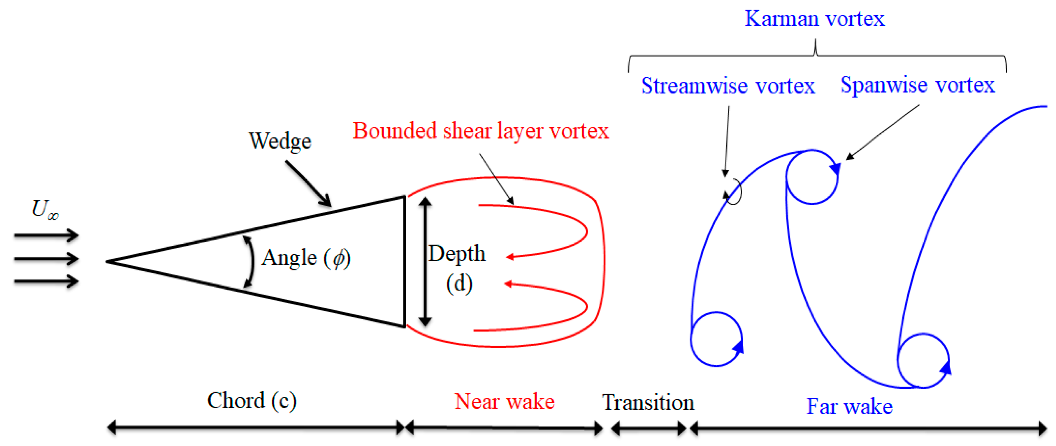
A two-dimensional wedge was adopted for the present study, as shown in Figure 1. The wedge was a triangle with the angle ($\alpha )$ of 15°, chord ($c$) of 75.96 mm, and depth ($d$) of 20 mm. The Reynolds number based on the free-stream velocity ($U_{\infty }$) and wedge depth ($d$) was $1.7\times {10}^5$. The cavitation number ($\sigma$) was defined as:

$$\sigma =\frac{P_0-P_v}{\frac{1}{2}\rho U_{\infty }^2}$$

(1)

where $P_v$ is the vaporization pressure and $\rho$ is the density of the fluid. The cavitation number was set to be 1.07, based on the free stream velocity and the outlet boundary’s reference pressure ($P_0$).

A low-pressure region was formed in the cavity behind the wedge. In the case of a low cavitation number, the outer cavity shape was seen steady even though there were the shear layer vortices inside. In the case of a high cavitation number, the cavity was convected downstream as the Karman vortices.

3. Computational Method and Validation

3.1. Incompressible Flow Solver

The equations for mass and momentum conservation were solved to obtain the pressure and velocity fields:

$$\nabla ·\left({\overrightarrow{{\rho }_{m}V}}_m\right)=0$$

(2)

$$\frac{\partial \left({\rho }_m{\overrightarrow{V}}_m\right)}{\partial t}+\nabla ·\left({\rho }_m{\overrightarrow{V}}_m{\overrightarrow{V}}_m\right)=-\nabla P+\nabla ·\overline{\tau }$$

(3)

where the subscript $m$ indicates the mixture phase and $P$ is the static pressure. The turbulent stress tensor $\overline{\tau }$ is also given by:

$$\overline{\tau }={\mu }_{eff}\left[\left(\nabla {\overrightarrow{V}}_m+\nabla {\overrightarrow{V}}_m^T\right)-\frac{2}{3}\nabla {\overrightarrow{V}}_m\overline{I}\right]$$

(4)

In Equation (4), the last term on the right-hand side represents the volume dilation effect, where ${\mu }_{eff}=\mu +{\mu }_t$ is the effective viscosity. The turbulence eddy viscosity (${\mu }_t$) is computed by combining $k$ and $\epsilon$ via ${\mu }_t={\rho }_m{C}_{\mu }{k}^2/ϵ$, and the turbulence kinetic energy (k) and the turbulence dissipation rate ($ϵ$) are obtained from the transport equations, which are:

$$\frac{\partial \left({\rho }_{m}k\right)}{\partial t}+\nabla ·\left({\rho }_{m}k{\overrightarrow{V}}_m\right)=\nabla ·\left[\left(\mu +\frac{{\mu }_t}{{\sigma }_k}\right)\nabla k\right]+G_k+G_b-{\rho }_mϵ-Y_M$$

(5)

$$\frac{\partial \left({\rho }_mϵ\right)}{\partial t}+\nabla ·\left({\rho }_mϵ{\overrightarrow{V}}_m\right)=\nabla ·\left[\left(\mu +\frac{{\mu }_t}{{\sigma }_{ϵ}}\right)\nabla ϵ\right]+C_{1ϵ}\frac{ϵ}{k}\left(G_k+C_{3ϵ}{G}_b\right)-C_{2ϵ}{\rho }_m\frac{{ϵ}^2}{k}$$

(6)

where $C_{\mu }$ is an empirical constant of 0.09. Here, the model constants $C_{1ϵ}$, $C_{2ϵ}$, ${\sigma }_k$, and ${\sigma }_{ϵ}$ are 1.44, 1.92, 1.0, and 1.3, respectively. The turbulence eddy viscosity was used to calculate the Reynolds stresses to close the momentum equations. The wall function was used for the near wall treatment [18].

The mixture density and also viscosity properties for both vapor and liquid were computed as functions of $\alpha$:

$${\rho }_m={\alpha }_v{\rho }_v+{\alpha }_l{\rho }_l$$

(7)

$${\mu }_m={\alpha }_v{\mu }_v+{\alpha }_l{\mu }_l$$

(8)

where $\alpha$ is the volume fraction and subscripts $v$ and $l$ indicate vapor and liquid, respectively. The Reynolds stress term was also related to the mean velocity gradient by the Boussinesq hypothesis, and the volume fraction transport equation was considered to account for the cavitation dynamics. The generation of cavitation was governed by the phase change dynamics in the system. The transport equation of two-phase mixture flow models could be expressed as follows:

$$\frac{\partial {\alpha }_v{\rho }_v}{\partial t}+\nabla ·\left({\alpha }_v{\rho }_v{\overrightarrow{V}}_m\right)=R_{cond}+R_{evap}+R_s$$

(9)

here the condensation term $\left(R_{cond}\right)$ and evaporation term ($R_{evap})$ can be expressed as:

$$R_{cond}=C_c\frac{v_{ch}}{\gamma }{\rho }_l{\rho }_l\sqrt{\frac{2}{3}\frac{P-P_v}{{\rho }_l}}{\alpha }_v$$

(10)

$$R_{evap}=C_e\frac{v_{ch}}{\gamma }{\rho }_v{\rho }_l\sqrt{\frac{2}{3}\frac{P-P_v}{{\rho }_l}}\left(1-{\alpha }_v\right)$$

(11)

where the condensation coefficient ($C_c$) and the evaporation coefficient ($C_e$) were set as 0.01 and 0.01, respectively [19]. $v_{ch}$ is the characteristic velocity and $\gamma$ is the surface tension.

3.2. Compressible Flow Solver

The homogeneous mixture equations with mass fractions were adopted to describe multiphase flows [20]. The continuity, momentum, and energy equations were used to describe the fluid mixture, whereas a single continuity equation was used for vapor and non-condensable gas phases. The conservative form of the compressible Reynolds-averaged Navier–Stokes equations was employed for an arbitrary control volume ($\mathsf{\Omega })$ with control surface ($\partial \mathsf{\Omega }$) as follows:

$$\frac{\partial }{\partial t}{{\displaystyle \int }}_{\mathsf{\Omega }}^{}\overrightarrow{W}d\mathsf{\Omega }+{{\displaystyle \oint }}_{\partial \mathsf{\Omega }}^{}\left[\left(F_C-F_v\right)·\overrightarrow{n}\right]dS={{\displaystyle \int }}_{\mathsf{\Omega }}^{}{\overrightarrow{Q}}_{pc}d\mathsf{\Omega }.$$

(12)

The vector of conservative variables ($\overrightarrow{\mathrm{W}})$ is given by:

$$\overrightarrow{W}={\left[\rho \rho u\rho v\rho w\rho E\rho y_v\rho y_g\right]}^T$$

(13)

where $\rho$, $E$, $y_v$, $y_g,$ and ($u, v, w$) are the mixture density, total energy, mass fraction of vapor phase, mass fraction of gas phase, and velocity vectors, respectively. $F_c$ and $F_v$ represent the corresponding convective flux vector and viscous flux vector, respectively. ${\overrightarrow{Q}}_{pc}$ is the vector of the phase change source term. The constitutive relation representing mass fraction was defined by:

$$y_l+y_v=1,$$

(14)

where the subscripts l, and v denote the liquid, and vapor phases, respectively.

The mixture density (ρ) and enthalpy (h) used in Equation (10) could be defined as:

$$\frac{1}{\rho }=\frac{\left(1-y_v\right)}{{\check{\rho }}_l}+\frac{y_v}{{\check{\rho }}_v}$$

(15)

here, ${\check{\rho }}_{}$ is defined by Amagat’s law.

The mixture enthalpy (h) was calculated as:

$$h=h_l\left(1-y_v\right)+h_v{y}_v.$$

(16)

The governing equations were closed with the inclusion of an equation of state for the constituent phases. All thermodynamic properties of each phase were generated as a function of local pressure and temperature. For each phase, various types of relations between the thermodynamic properties (ρ, h) and independent variables (p, T) were used [13].

The same turbulence and cavitation models used for the incompressible flow solver were applied to the compressible flow solver. The model constants for the cavitation model were also identical.

3.3. Solver Validation

To validate both of the developed solvers, the sheet cavitation around a hemispherical head-form body and a modified NACA66 hydrofoil was simulated. Rouse and McNown [21] carried out experiments on the natural cavitating flow around a cylindrical body with a hemispherical head-form shape. The pressure coefficient ($C_P)$ was defined as:

$$C_P=\frac{P-P_o}{\frac{1}{2}\rho U_{\infty }^2}$$

(17)

The freestream inlet velocity $(U_{\infty }^{})$ was set to be 0.7 m/s. The cavitating flow around a hemispherical head-form body was simulated at the cavitation number of 0.2 and the Reynolds number of $1.36\times {10}^5$ [2]. Figure 2 shows the volume fraction contours around the hemispherical head-form body by both solvers. In the incompressible flow solution, a short re-entrant jet was observed near the cavity closure. In the compressible flow solution, a longer re-entrant jet was seen up to the mid-cavity point. The longer cavity length by the compressible flow solver was seen due to the re-entrant jet. Figure 3 shows the pressure coefficient distribution on the hemispherical head-form body surface by both solvers and experiments. The pressure overshoot at the cavity closure was more prominent in the incompressible flow solution.

The cavitating flow around the modified NACA66 hydrofoil with the angle of attack of $4^{\mathrm{o}}$ was simulated at the cavitation number of 0.84 and the Reynolds number of $2\times {10}^6$ [19]. Figure 4 shows volume fraction contours around the modified NACA66 hydrofoil by both solvers. In the incompressible flow solution, the cavity was closed smoothly. In the compressible flow solution, on the other hand, a re-entrant jet was observed near the cavity closure. Figure 5 shows the pressure coefficient distribution on the modified NACA66 hydrofoil surface by both solvers and experiments [22]. The pressure coefficients were similar in most of the region except near the cavity closure. By comparing with the experimental data, it was confirmed that the pressure coefficient by the compressible flow solver was more accurate compared to that by the incompressible flow solver at the cavity closure.

4. Results and Discussion

In the Cartesian coordinate system adopted here, the positive x-axis was in the streamwise direction, and the positive y-axis was in the vertical direction. The solution domain extent was −30 < x/c < 41 and −30 < y/c < 30. The left inlet boundary was specified as the Dirichlet boundary condition, i.e., with a fixed value of the inflow velocity. On the exit boundary, the reference pressure with the extrapolated velocity and the volume fraction were applied. The no-slip condition was applied on the wedge surface. A C-type structured grid consisted of 11,900 cells, i.e., 170 cells on the body and 70 cells in the normal direction, was used [2].

The time step size of 10⁻⁶ was selected, which corresponded to the Courant number of 0.5. The simulation time was advanced when the normalized residuals for the solutions had been dropped by six orders of magnitude.

4.1. Cavity with Bounded Shear Layer Vortices

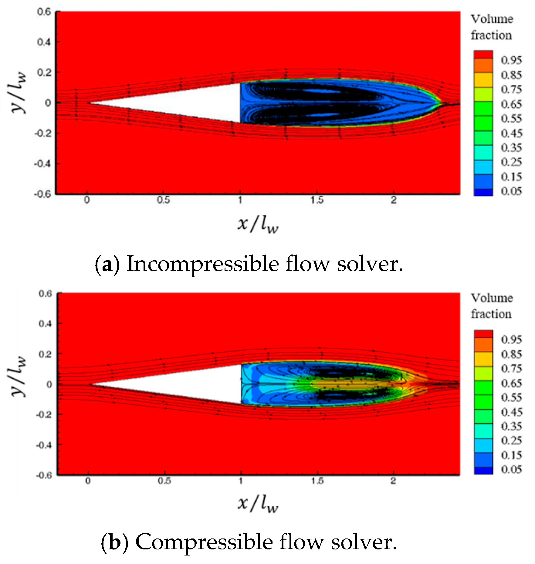
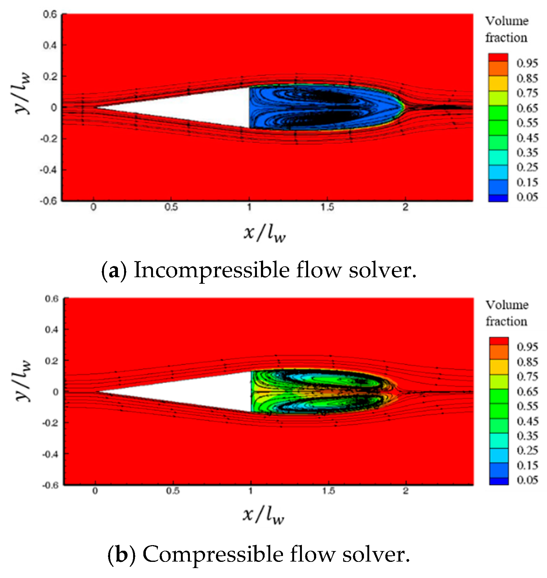
Simulations at the low cavitation numbers of 0.35 and 0.4 and the Reynolds number of 1.7 × 10⁵ were carried out by both solvers. In the low cavitation number case, flow fluctuation over time was reduced quickly and thereby the cavity shedding was not observed. Figure 6 and Figure 7 show the volume fraction contours and streamlines around the two-dimensional wedge at cavitation numbers of 0.35 and 0.4, respectively. The bounded shear layer vortices were seen in the cavity from the streamlines and the re-entrant jet was not observed in the incompressible flow solution. The core of the bounded shear layer vortices was seen at mid-cavity. On the other hand, in the compressible flow solution, the core was seen near the cavity closure. The re-entrant jet was clearly reproduced by the compressible flow solver. The core of the bounded shear layer vortices was also influenced by the re-entrant jet. The re-entrant jet, which generated near the cavity closure, was the cause of the shorter cavity length in the compressible flow solution.

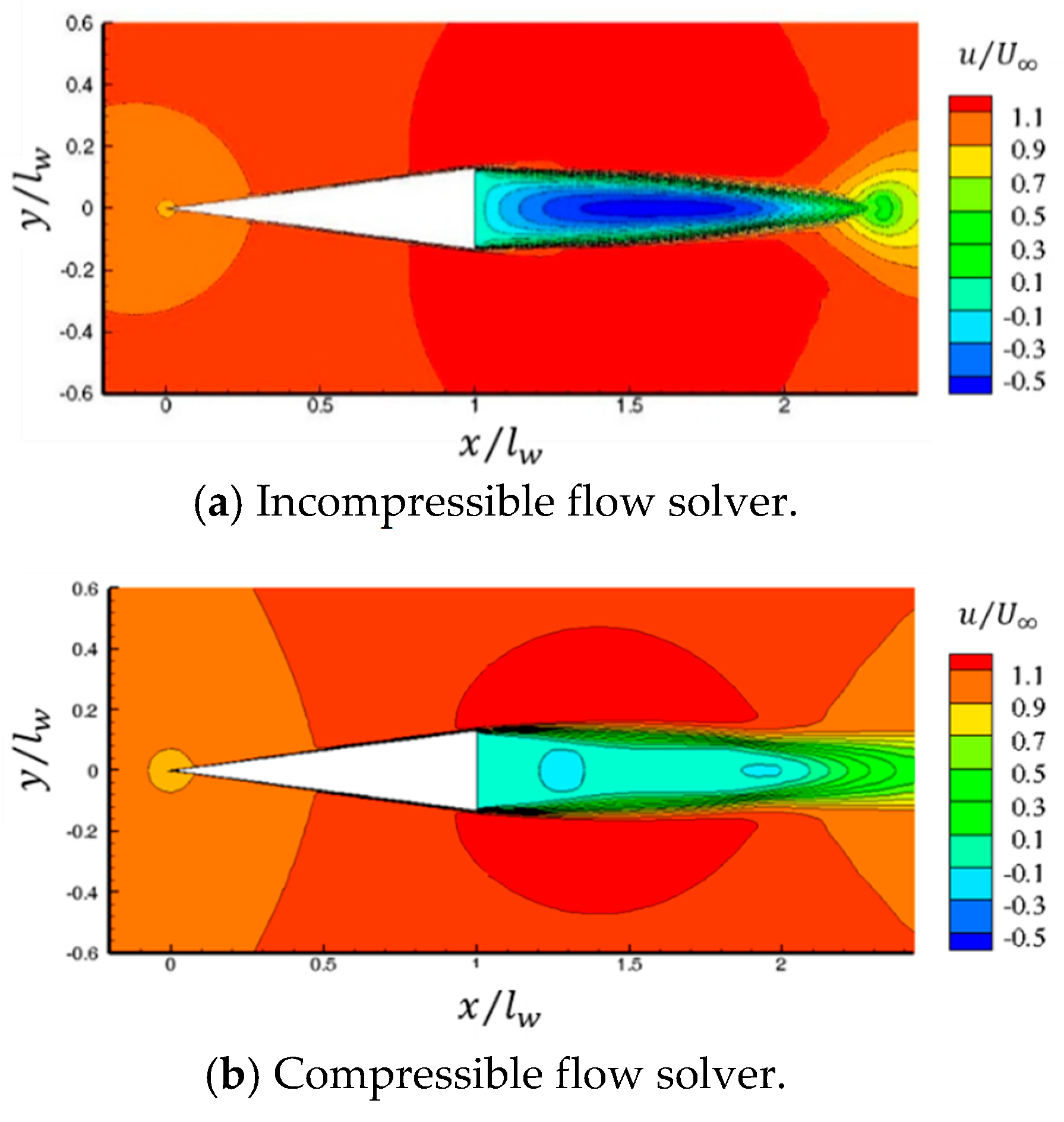
Figure 8 and Figure 9 show the contours of non-dimensionalized streamwise velocity component around the wedge at the cavitation numbers of 0.35 and 0.4, respectively. A negative streamwise velocity at the centerline was seen due to the bounded shear layer vortices. The minimum negative non-dimensionalized streamwise velocity component of −0.5 by the incompressible flow solver was rapidly changed near the cavity closure because the cavity and freestream were disconnected by a cavity interface. That by the compressible flow solver was the relatively bigger value of −0.1 and slowly changed near the cavity closure because of the re-entrant jet.

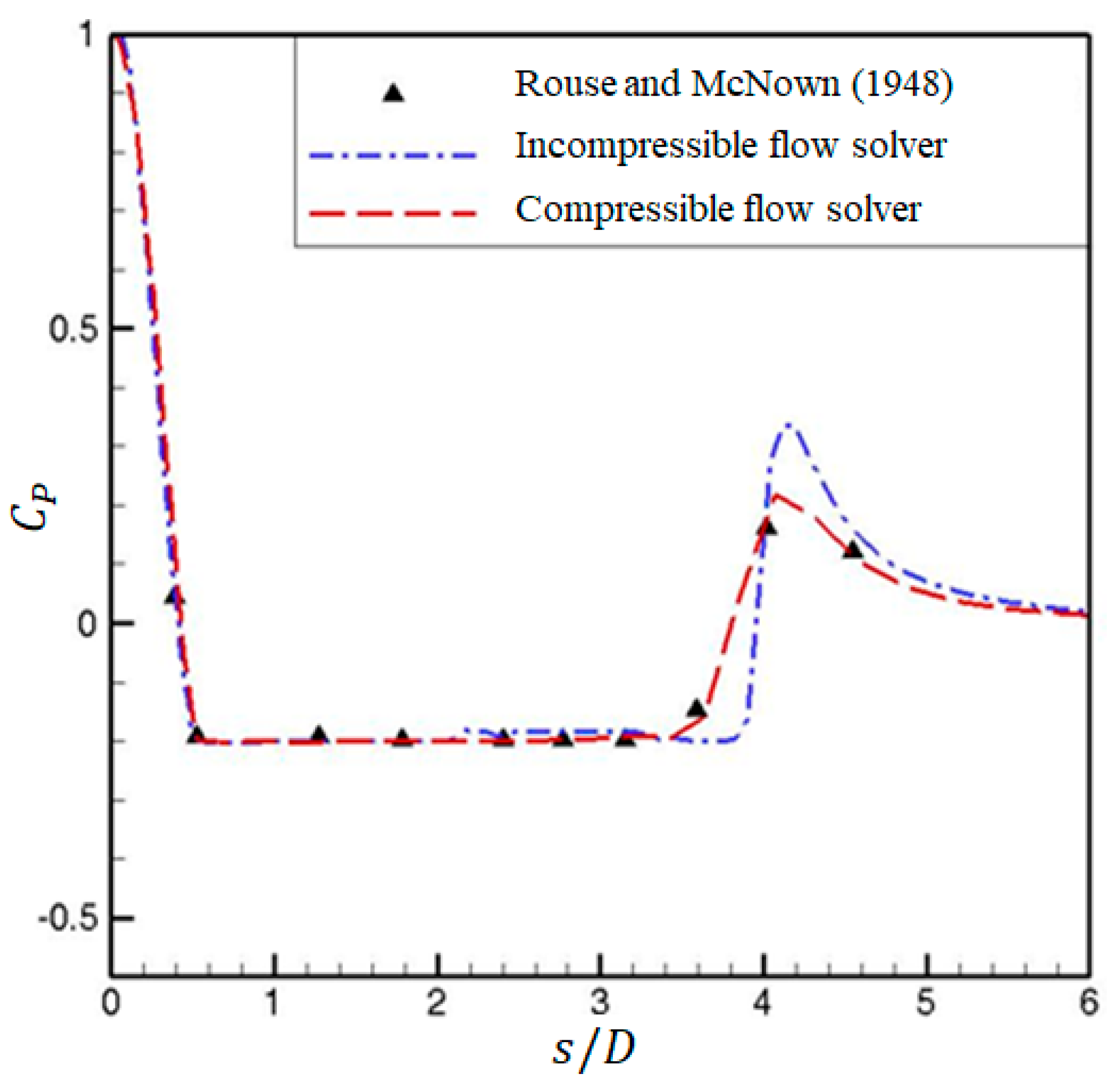
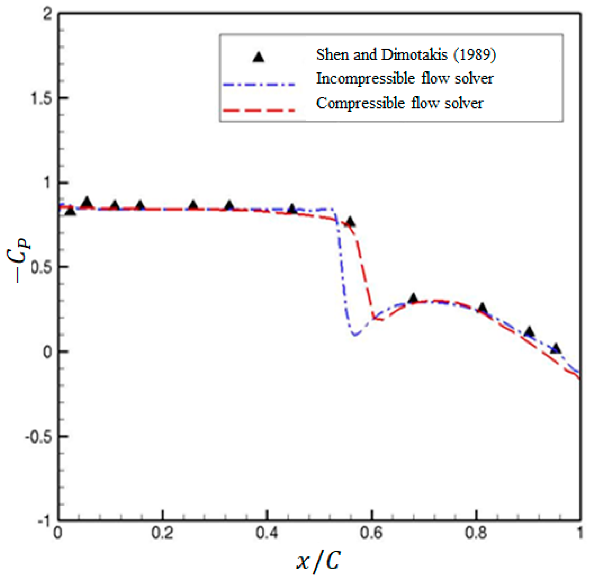
Figure 10 and Figure 11 show the pressure coefficient contours around the wedge at the cavitation numbers of 0.35 and 0.4, respectively. In the compressible flow solution, the pressure was slowly changed near the cavity closure due to the re-entrant jet. While, in the incompressible flow solution, the pressure was rapidly changed near the cavity closure and even showed high value after the cavity closure. Those were because there was no interaction between the cavity and outer flow by the re-entrant jet. The pressure overshoot at the cavity closure shown in Figure 3 and Figure 5 was also caused by the rapid pressure change in the incompressible flow solution.

The cavity lengths predicted by both solvers were compared with the experimental results. The experimental observations were carried out in the cavitation tunnel at Chungnam National University. The cross-section size of the tunnel’s test section was 100 mm wide and 100 mm high. The maximum speed of the tunnel free stream was 20 m/s and the pressure was controlled from 10 to 300 kPa. Figure 12 is a snapshot of the cavity behind the wedge at the cavitation numbers of 0.35 and 0.4 and the Reynolds number of 1.7 × 10⁵. The observed non-dimensionalized cavity lengths (l_c/d) in the experiments were 5.45 and 3.84 at the cavitation numbers of 0.35 and 0.4, respectively. The cavity lengths predicted by both solvers were shorter than that by the experiments. In the experiment, it was presumed that the cavity length was longer than that by the incompressible and compressible flow solvers due to the impurity of the water. A longer cavity was predicted by the incompressible flow solver and the re-entrant jet was clearly observed in the compressible flow solution. The re-entrant jet was the cause of the shorter cavity length in the compressible flow solution.

The computed cavity lengths were compared with the experimental results and analytic solution [23], as shown in Figure 13. The cavity lengths were calculated using a vapor volume fraction value of 0.5. The cavity length and re-entrant jet grew longer as the cavitation number decreased. The cavity lengths predicted by both solvers were somewhere between the experimental data and analytic solution. The analytic solution was based on the potential flow. The lack of viscosity could cause a shorter cavity length. The cavity lengths computed by the incompressible flow solver were longer than that by the compressible flow solver because the re-entrant jet in the compressible flow solution caused the cavity length to be shortened. The impurity of the water in the experiment caused the longer cavity length than that by both solvers. This tendency was prominent at a low cavitation number.

4.2. Cavity with Karman Vortices

To observe the cavity shedding dynamics, simulations at a high cavitation number of 0.83 were performed. Cavity shedding was observed at the cavitation number of 0.83 and the Reynolds number of 1.7 × 10⁵. On issues such as cavity shedding, the shedding is related to the Reynolds number, while the cavity is related to cavitation number. Figure 14 shows the volume fraction contours and streamlines. The Karman vortices were repeated with period $T$, and $t_o$ was an arbitrary time. The Karman vortices were identified at both cases from the streamlines. At $t=t_o+T/2$, the Karman vortex from the upper side moved downstream and the lower Karman vortex rolled up. The cavity length at the centerline in the incompressible flow solution was longer than that in the compressible flow solution. It indicated that the transition from the bounded shear layer vortices to the Karman vortices was generated rapidly in the incompressible flow solution.

5. Concluding Remarks

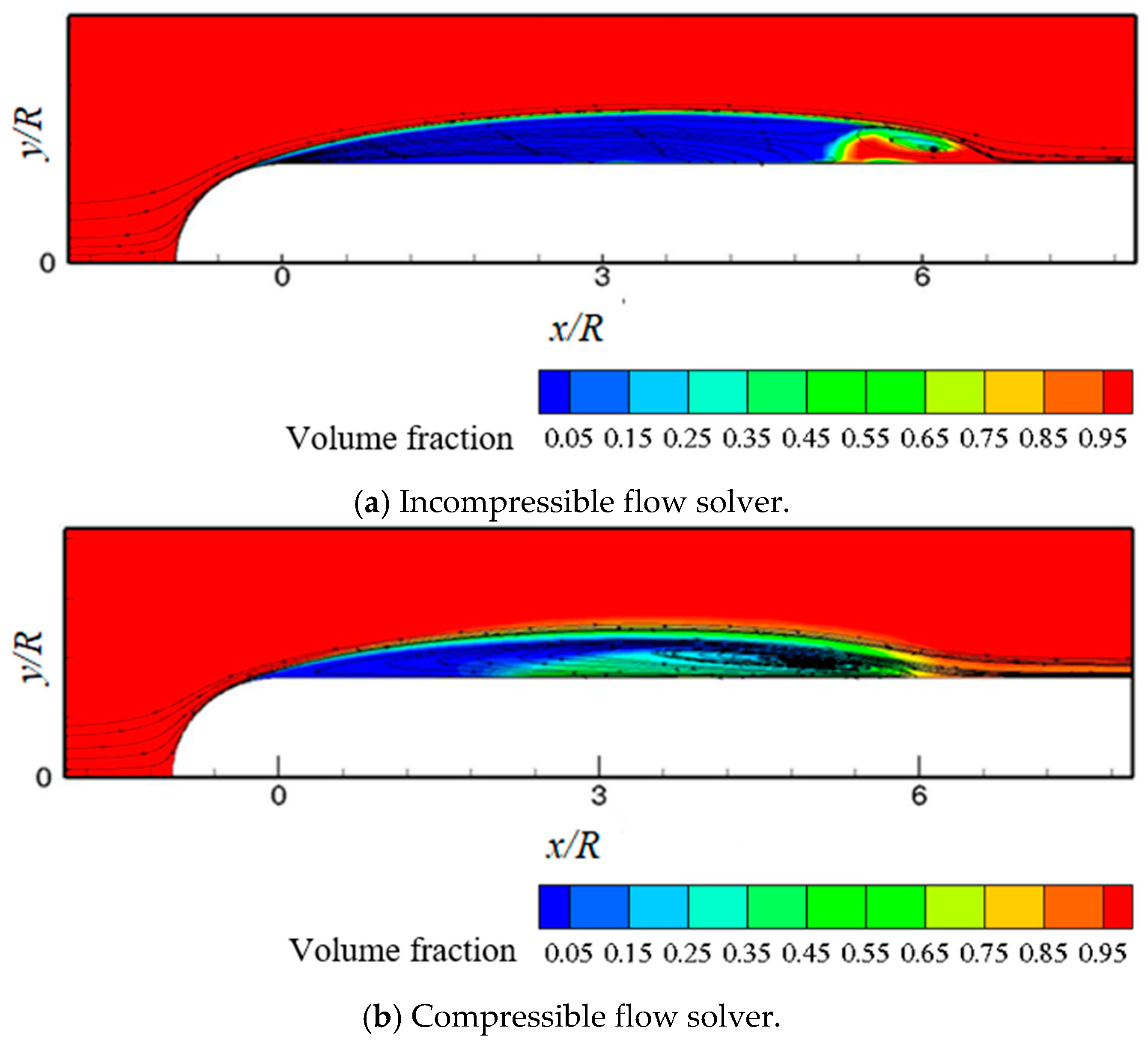
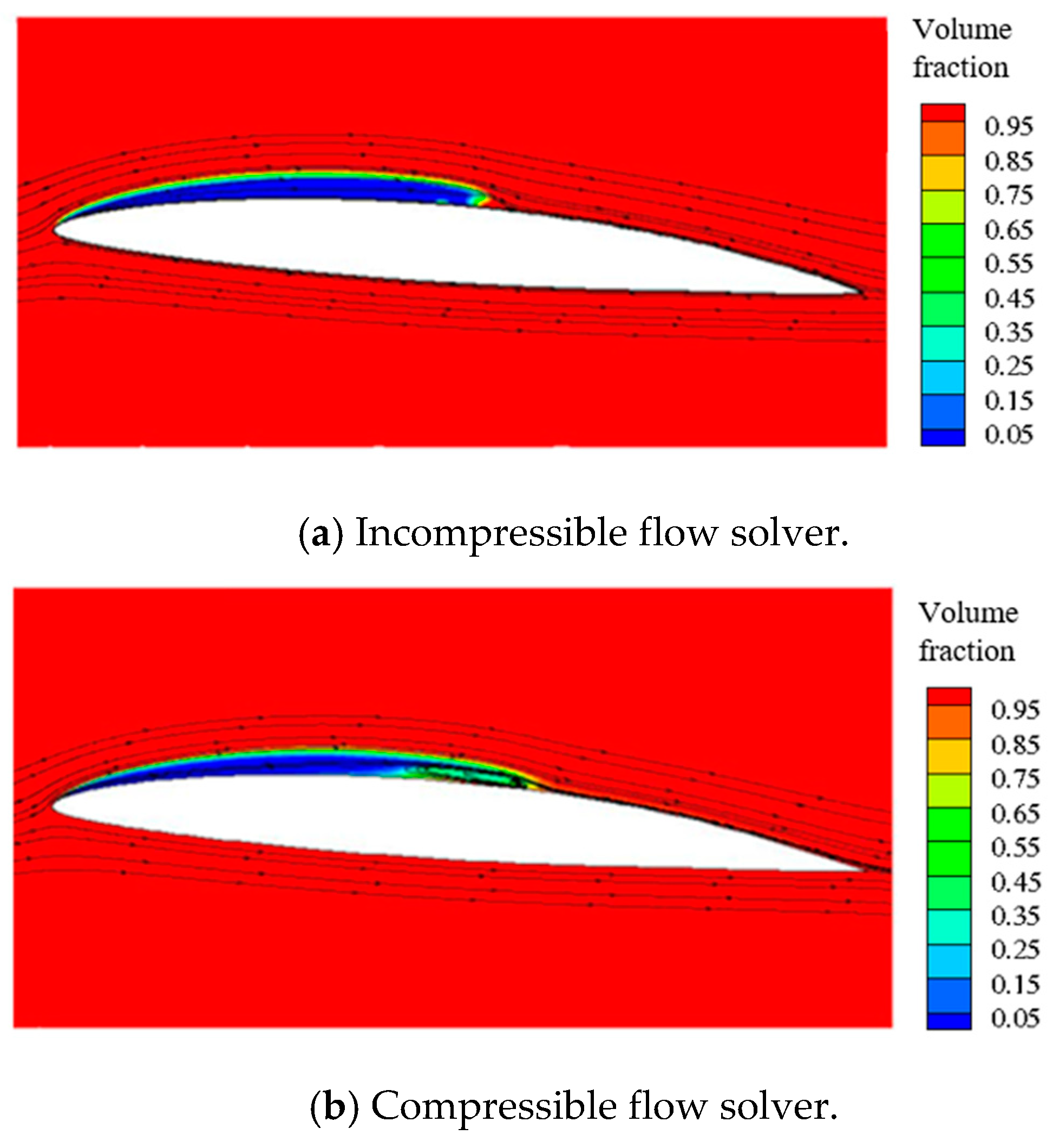
To investigate the compressibility effect for external cavitating flows, pressure-based incompressible and density-based compressible flow solvers were developed, respectively. Both solvers were validated by applying to cavitating flows around a hemispherical head-form body and the modified NACA66 hydrofoil.

The cavitating flow behind a wedge by both solvers was studied. In comparison to the computational results, experiments were carried out in the cavitation tunnel at Chungnam National University. At the low cavitation numbers of 0.35 and 0.4, the cavitating flow with the bounded shear layer vortices and cavity lengths was similar in both solutions. The re-entrant jet was captured by the compressible flow solver. The re-entrant jet caused a relatively slow change of the pressure and velocity near the cavity closure. In the incompressible flow solution, the pressure and velocity were changed rapidly near the cavity closure because there was no interaction between the cavity and outer flow by the re-entrant jet. At the cavitation number of 0.83, both solvers captured the transition from bounded shear layer vortices to Karman vortices. The re-entrant jet in the compressible flow solution caused a shorter cavity length. From the Karman vortices, the transition was more rapidly progressed in the incompressible flow solution.