Review

Efficient Nonlinear Hydrodynamic Models for Wave Energy Converter Design—A Scoping Study

1
Department of Fluid Mechanics, Faculty of Mechanical Engineering, Budapest University of Technology and Economics, 1111 Budapest, Hungary
2
Wave Venture Ltd., Truro TR4 8PN, UK
*
Author to whom correspondence should be addressed.
J. Mar. Sci. Eng. 2020, 8(1), 35; https://doi.org/10.3390/jmse8010035
Submission received: 30 November 2019 / Revised: 1 January 2020 / Accepted: 3 January 2020 / Published: 11 January 2020
(This article belongs to the Special Issue Nonlinear Numerical Modelling of Wave Energy Converters)

Abstract

:
This review focuses on the most suitable form of hydrodynamic modeling for the next generation wave energy converter (WEC) design tools. To design and optimize a WEC, it is estimated that several million hours of operation must be simulated, perhaps one million hours of WEC simulation per year of the R&D program. This level of coverage is possible with linear potential flow (LPF) models, but the fidelity of the physics included is not adequate. Conversely, while Reynolds averaged Navier–Stokes (RANS) type computational fluid dynamics (CFD) solvers provide a high fidelity representation of the physics, the increased computational burden of these models renders the required amount of simulations infeasible. To scope the fast, high fidelity options, the present literature review aims to focus on what CFD theories exist intermediate to LPF and RANS as well as other modeling options that are computationally fast while retaining higher fidelity than LPF.

1. Introduction

The development of commercial WEC technology is a complex and challenging endeavor. Weber et al. [1] outlined an improved WEC technology development methodology, by introducing a novel Technology Performance Level (TPL) metric to complement the more widely used Technology Readiness Level (TRL) metric (depicted in Figure 1a), and detail an overall R&D management philosophy that is tailored to the challenges of WEC development. Work following from [1] has focused on the development of the TPL metric [2], on a combination of the new approach with the discipline of Systems Engineering [3], on the application of the TRIZ Structured Innovation methodology [4], and on the risk analysis for WEC product development [5]. This paper explores one of the other needs identified in [1], namely the need for reliable, robust, and affordable simulations of WEC technology.

1.1. R&D Context for WEC Simulation

The WEC R&D management philosophy described in [1], may be termed the Performance before Readiness philosophy. Pursuing a Performance before Readiness approach reduces the cost of product development and increases the probability of market entry. A central component of this approach is making performance improvements at early stages in the R&D program by maintaining the flexibility of concept and conducting evaluation and optimization of many alternative concepts, while still at low TRL (depicted by trajectory A in Figure 1b). Conversely, the alternative Readiness before Performance approach (depicted by trajectory B in Figure 1b), reduces the probability of market entry and, in wave energy, virtually guarantees bankruptcy [1].
Making performance improvements requires reliable and affordable performance estimates, which brings WEC simulation into the spotlight. It is uneconomical to obtain performance estimates, for a wide diversity of concepts at low TRL, using a program that relies exclusively on experimentally derived results. Software simulation is one of the key enabling technologies that will facilitate the Performance before Readiness approach.

1.2. Requirements of WEC Simulation

A particular need is a WEC simulation that is suitable for automatic optimization. Techno-Economic (combined engineering and financial) optimization, is specifically anticipated in [1], but any kind of WEC optimization, with or without financial objective functions, still requires a WEC simulation that is suitable for automatic optimization. To be suitable for automatic optimization, a simulation must satisfy the following requirements:
(a)
Fidelity requirement—be reliable for all possible trial vectors that an optimization algorithm might generate for evaluation,
(b)
Flexibility requirement—be general enough to be applicable to a wide variety of candidate WEC concepts, and
(c)
Computational requirement—be fast/affordable enough to allow sufficient generations or iterations to be completed in practical time scales on available and affordable hardware.

1.3. Objective of Scoping Study

Arguably none of the well established WEC simulation approaches satisfy all the requirements for an ideal simulation tool for WEC design. Most approaches to WEC simulation can be characterized by a position on a speed-fidelity spectrum. One extreme of the spectrum is high speed but low fidelity, while the opposite extreme of the spectrum is low speed but high fidelity. The two well-established approaches to WEC simulation occupy these opposite extremes:
  • At the low-fidelity/high-speed end of the spectrum are methods based on LPF, including frequency-domain methods [6], Cummins equation time-domain methods [7], and extensions of Cummins methods, such as the Nonlinear Froude–Krylov (NLFK) approach (see Section 3.6.2).
  • At the high-fidelity/low-speed end of the spectrum are approaches based on RANS CFD codes (see review in [8]). Schmitt et al. [9] present the challenges and advantages for the application of RANS-based methods in the design process of a WEC, concluding the major drawback is the significant computational power required.
Mature software packages, both commercial and open-source, based on the opposite extremes of the speed-fidelity spectrum are available and their properties are relatively well known. It is the contention of the authors that neither of these mature approaches satisfies the requirements for an ideal WEC simulation tool, the fast methods are not accurate or robust enough and the accurate methods are not fast or affordable enough. We propose that a specialist WEC simulation tool based on an intermediate CFD theory is needed. CFD Theories that are intermediate to LPF and RANS exist, but compared to LPF and RANS are relatively under-developed with few commercial or open-source software products available and knowledge of the properties of these approaches is often only available to the creators of research codes. In this paper, we set out to review the CFD theories and related methods that are intermediate to LPF and RANS with a view to identifying promising avenues for a specialist WEC simulation tool.

1.4. Previous Reviews

A very early comparison of numerical methods in free-surface hydrodynamics can be found in Yeung [10] from the Hydrodynamics of Ocean Wave-Energy Utilization Symposium in 1985. Nearly three decades later, in 2012, Li and Yu [11] reviewed the modeling methods available for point absorber type WECs. In the same year, Folley et al. [12] reviewed hydrodynamic modeling for WEC arrays, which were again later reviewed in DeChowdhury et al. [13]. Nonlinear hydrodynamic modeling of WECs is the focus of the reviews in Wolgamot and Fitzgerald [14] and Penalba et al. [15], whereas the reviews in Windt et al. [8] and Zullah et al. [16] specifically focus on RANS modeling of WECs. Zabala et al. [17] review integrated approaches to numerical and experimental testing, from full-scale prototype and physical wave tank (PWT) models to RANS and LPF simulations. Saincher and Banerjee [18] review the influence of wave breaking on WEC hydrodynamics. Whereas the reviews in Coe et al. [19,20] focus on the modeling methods for WEC survival in extreme seas. In addition, a good book detailing the current state-of-the-art in WEC hydrodynamic modeling was recently published in 2016 [21].

1.5. Outline

Mathematical modeling of nonlinear WEC hydrodynamics require a venture from physics to numerics. Increasing the computational efficiency can, therefore, be pursued through prudent selection of the relevant physical effects to be modeled, a parsimonious mathematical description of the selected effects and an efficient numerical scheme to solve the governing equations. Considering the physics, Section 2 presents the different types of nonlinear hydrodynamic effects a WEC may be subjected to and the conditions under which these effects are relevant. Next, turning to the mathematics, the governing system of equations for fluid dynamics, the Navier–Stokes equations (NSE) are introduced and their role in hydrodynamic modeling for WECs discussed. The spectrum of numerical schemes, with varying complexity and fidelity, utilized to solve the NSE are then presented to set the scene for the following sections, which collate and review the literature, laid out as follows:
  • Section 3 reviews the CFD theories intermediate to RANS and LPF, which simplify the NSEs yet retain the potential to simulate nonlinear WEC hydrodynamics.
  • Section 4 reviews the use of Domain Decomposition, which aims to reduce the required computational overhead of high fidelity CFD codes, by simulating the bulk of the computational domain with a lower fidelity model with fast computational speed, while only simulating the area in the immediate vicinity of the WEC with computationally expensive, higher fidelity models.
  • Section 5 then reviews computationally fast modeling techniques, capable of simulating WEC performance with a high fidelity that includes nonlinear effects, but at a fraction of the computational cost of the NSE-type CFD simulations reviewed in Section 3 and Section 4.
Section 6 discusses the main points gathered from Section 3, Section 4 and Section 5, in particular, those methods which have the potential of performing efficient simulations to aid in WEC design, and provides a tabulated comparison of the different methods reviewed. Conclusions are presented in Section 7.

2. Efficient Nonlinear Hydrodynamic Models for WECs

A good description of WEC hydrodynamics is given in Todalshaug [22], detailing the fundamental principles of wave absorption and hydrodynamic forces on bodies. The traditional modeling approach treats the hydrodynamic forces linearly (see Falnes [23] for an in-depth description), for time domain [7] and/or frequency domain [6] analyses of the WEC based on LPF. Correspondingly, this type of modeling approach leads to a linear relationship between the input wave and the output WEC motion. Thus, if the wave height is doubled, the resulting amplitude of WEC motion also doubles. However, in reality, this does not hold for a large portion of the simulations required for WEC design, due to nonlinear effects. Section 2.1 discusses the types of nonlinearities which can appear during WEC operation and Section 2.2 details the factors which influence the prevalence or absence of these nonlinearities in WECs. Modeling these nonlinearities requires a more thorough treatment of the NSE, without the full range of linearing assumptions inherent to LPF, as detailed in Section 2.3.

2.1. Hydrodynamic Nonlinearities—Types

There are three main physical effects, neglected in the linear formulation, which give rise to hydrodynamic nonlinearities: viscosity, nonlinear waves, and time-varying wetted body surface. The nonlinear viscous effects are omitted in the linearization of the equations, discussed in Section 3.1.1, whereas the effects of the nonlinear waves and time-varying wetted body surface are omitted in the linearization of the boundary conditions, as discussed in Section 3.1.2.

2.1.1. Viscosity

Viscosity gives rise to drag forces, resulting from pressure/form drag and skin friction drag. For WECs, pressure drag is the main contributor and skin friction is typically negligible [22]. Pressure drag is caused by flow separation and vortex shedding, whose force on the WEC is nonlinear, increasing quadratically with the relative WEC-water velocity.
In marine hydrodynamics, the relative importance of viscous forces increases as the size of the body decreases [24]. Therefore, in many offshore engineering applications, neglecting viscous effects to enable a linear formulation of hydrodynamics is a valid approximation, owing to the large size of the structures, such as ships and floating oil platforms. For WECs however, the characteristic lengths are generally much smaller and the role of viscosity can be important. WECs also differ from most offshore structures, in that they are designed to resonate with the input waves, whereby the large amplitude wave-driven motions result in increased relative WEC-water velocity.
Neglecting viscosity in WEC analysis results in an underestimation of the hydrodynamic damping, leading to predictions of unrealistically large WEC motions and energy capture, especially around resonance [25] and when driven by an energy maximizing control system [26,27]. This is exemplified in Figure 2, from the case study in [26], showing the overestimation of the WEC motion predicted by a linear Cummins equation model, compared to a RANS simulation, when a control system uses the power take-off (PTO) to drive a heaving point absorber (HPA) into resonance with the input waves, contrasted against the case where no control is applied and the device is not in resonance.

2.1.2. Nonlinear Ocean Waves

Figure 3 shows that linear theory is only valid in deep and intermediate water depths for small amplitude waves. As the relative water depth decreases and/or the relative wave height increases (relative with respect to the wave length), then the linear theory breaks down and the wave becomes nonlinear. Wave breaking, as an extreme case, is a very nonlinear process (see review in Saincher and Banerjee [18]). The difference in loads calculated including the wave nonlinearity versus the loads calculated by purely linear models is important for load design and survival and is examined by Viuff et al. [28] for the case of the Wavestar WEC. Additionally, the wave nonlinearity affects the hydrodynamic efficiency of a WEC. For example, Ning et al. [29] show that the hydrodynamic efficiency of a fixed oscillating water column (OWC) attains a maximum value at a critical wave slope and decreases when the wave nonlinearity becomes either stronger or weaker. Giorgi and Ringwood [30] examine the effect of wave nonlinearity on the calculation of Froude–Krylov (FK) forces on an HPA and an oscillating surge converter (OSC) for the different sea states occurring at the European Marine Energy Centre, contrasting the degree of error with the likelihood of the sea state occurrence. Further discussion on wave nonlinearity is given in Section 6.3.

2.1.3. Time-Varying Wetted Body Surface

The hydrodynamic force on a WEC results from the integral of the fluid pressure over the wetted-surface area. For a linear model, the wetted surface area is assumed constant, calculated at the equilibrium position, and the forces linearized around that point, such that a doubling in wave elevation, body displacement, or velocity, equals a doubling in the wave excitation force, hydrostatic restoring force or radiation force, respectively. This is illustrated in Figure 4, for the hydrostatic restoring force on a sphere and a cone, as a function of the heave displacement, showing the actual nonlinear result due to the time-varying wetted body surface and the linearized version. The time-varying wetted body surface, and resulting time-varying system parameters, can lead to phenomena such as parametric resonance [32,33,34,35,36]. In some cases, the geometry of the WEC may also change with time. Examples of these are flexible structures such as the Bombora, the Anaconda, and the WECs investigated in [37,38], or WECs with movable control surfaces such as in Diamond et al. [39] and Tom et al. [40].

2.2. Hydrodynamic Nonlinearities—Dependences

The influence of the different types of hydrodynamic nonlinearities, detailed in Section 2.1, varies on a case by case basis, dependent on the following:

2.2.1. Device Dependence

Hydrodynamic nonlinearities are device-dependent. For example, Folley et al. [41] contrast the hydrodynamics of heaving and surging devices and conclude that the hydrodynamics of the two are very different and should be considered distinctly. Similarly, Giorgi and Ringwood [42] compare the relative importance of different hydrodynamic forces for HPAs and OSCs, and show that HPAs are predominately affected by NLFK forces, whereas, for OSCs, the diffraction and radiation effects are the most important. For the case of OWCs, the review in [14] identifies that the effects of viscosity appear to be significantly larger than nonlinearities associated with the waves or time-varying wetted surface, particularly at resonance. [15] reviews the relevant importance of nonlinear hydrodynamic effects in OWCs, HPAs, OSCs, and oscillating pitch converters, highlighting differences between each.

2.2.2. Sea State Dependence

The hydrodynamic nonlinearities can depend on the sea states. Sea states with peak frequencies aligned with the WEC natural frequency will result in large amplitude, resonant WEC motion, enhancing both viscous and time-varying wetted body nonlinear effects. For example, Yu and Li [25] show large discrepancies between linear models and RANS simulations, for input waves corresponding to the resonance frequency of the WEC, but a closer agreement for other frequencies. Additionally, sea states with larger wave heights are more likely to have waves that fall outside of the linear region in Figure 3. Wang et al. [43] investigate the effect of the wave nonlinearity and viscosity on the performance of an OWC, by comparing the linear and nonlinear numerical results and show the changing relative importance of these nonlinear effects as the wave amplitude increases. Furthermore, the wave nonlinearity could also depend on the tide, with shallower water depths at low tides increasing the likelihood of waves falling outside of the linear region in Figure 3.

2.2.3. Control Dependence

The relevance of different nonlinear effects can also depend on the control applied to the device [26,27]. For example, Giorgi and Ringwood [27] examine hydrodynamic nonlinearities in controlled versus uncontrolled conditions for a spherical HPA. The accuracy and computation time of eight different partially nonlinear models are compared against RANS simulations, for cases with and without latching control in regular waves. The results show that when no latching is applied, nonlinearities were not significant, however, with control, NLFK and viscous drag forces become relevant. Similar results are shown in Davidson et al. [26] for an HPA in a JONSWAP spectrum, with and without a controller applying reactive power through the PTO.

2.2.4. Scale Dependence

Hydrodynamic nonlinearities are also scale-dependent. This can be important to consider given that the assessment hydrodynamic model success is often with respect to physical models at the laboratory scale. Therefore, it is also important to understand the effects of scaling on the relative importance of nonlinear hydrodynamic forces, as discussed in Fitzgerald [44]. For example, this point is examined in Schmitt and Elsaser [45], considering the applicability of Froude scaling from PWT to full-scale OSCs using both tank tests and RANS simulations. The effect of scaling PWT results for a moored HPA, from 1:10 to full scale, is investigated in Windt et al. [46], through the use of upscaling. In the review De Chowdhury et al. [13], specific emphasis is paid on understanding how the modeling and scaled experiments are likely to be complementary to each other. See Palm et al. [47] also in Section 3.2.

2.3. The Navier–Stokes Equations

Accurately modeling the nonlinear wave-structure interaction (WSI), requires a thorough treatment of the hydrodynamic interaction between the WEC and the fluid, which can be obtained via an appropriate application of the NSE. The NSE are a set of partial differential equations, describing the dynamics of fluids, through the conservation of mass and momentum:
ρ ( x , t ) t + · ρ ( x , t ) U ( x , t ) = 0 ,
ρ ( x , t ) U ( x , t ) t + U ( x , t ) · ρ ( x , t ) U ( x , t ) = p ( x , t ) + · T ( x , t ) + ρ ( x , t ) f b ( x , t ) ,
where x denotes the three-dimensional (3D) spatial coordinate, t the time, U the fluid velocity, p the fluid pressure, ρ the fluid density, T the stress tensor, and f b external forces, such as gravity.

2.3.1. Solving

This first thing to note when solving the NSE is that there are four equations (the momentum equation consists of a separate equation for each of the three spatial directions), with five unknowns (pressure, density and the three velocity components). Therefore, an additional equation is required to enable closure. To achieve this, the conservation of total energy is used to yield “the energy equation”, which introduces a sixth unknown (temperature), and then an “equation of state” is used to give six equations with six unknowns (see Ferziger and Peric [48] for more details).
In general, the NSE have no known analytical solution, however, they may be treated numerically to obtain a solution. To solve the NSE, the continuous partial differential equations are discretized into a system of linear algebraic equations, which can then be solved by computer. That is, the continuum is broken up into finite temporal and spatial portions to transform a calculus problem into an algebraic problem. The problem can be discretized temporally using timesteps. Spatially, a number of different methods are available for the discretization:
  • Mesh: A common approach, which is the main focus of the models reviewed in Section 3, discretizes the domain into nodes/cells.
  • Particles: Discretizes the domain into lagrangian particles, via methods such as smoothed particle hydrodynamics (SPH) (discussed in Section 4.4).
  • Particle distribution field: Discretizes the domain into a field giving a statistical representation of the particle distribution using methods such as Lattice Boltzman (LB) (discussed in Section 4.5).
The pyramid in Figure 5 depicts the increase in accuracy versus the spatial and temporal discretizations, represented by the number of model parameters and the simulation time step, respectively. The higher up the pyramid the more accurate the solution (probably on a log-scale for WEC simulations) and the smaller the cross-sectional area of the pyramid, at a given height, the greater the computationally expense (probably on an exponential scale for WEC simulations).

2.3.2. Methods

At the top of the pyramid in Figure 5, the most accurate and computationally expensive way to solve the NSE is through direct numerical simulation (DNS), where all dynamics generated from the NSE are simulated on all spatial and time scales. This requires such a high spatial and temporal resolution, that the enormous number of model parameters and the minuscule simulation time steps prohibit DNS from being applied to WECs. To overcome this, large-eddy simulation (LES) and RANS methods model some of the physics rather than directly resolving the smallest scale phenomena.
For LES, the large scale turbulent structures are directly resolved and the turbulence on the sub-grid scale is modeled, which is still very computationally expensive, and has therefore rarely been applied to WEC applications (examples of LES applied to WECs can be seen in [52,53,54]). The RANS method does not attempt to directly resolve any of the turbulent structures, thus larger mesh cells and time steps are possible, which significantly reduces the computational requirements of this method compared to DNS and LES. RANS modeling is, therefore, becoming more computationally accessible (in line with the increased availability of low cost— high-performance computers) and is growing in popularity, with a recent review collating over 200 publications that apply RANS modeling for WECs [8]. However, as noted in Section 1.1, RANS is still too computationally expensive to simulate multiple WEC design iterations across multiple sea states.
At the bottom of the pyramid are linear hydrodynamic models based on the Cummins equation [55]. For these linear Cummins models, the simulation time step can be equal to the sampling of a sea state (approx. 30 mins) using frequency domain analysis [7] and the number of model parameters on the order of the number of frequency components considered. The white region on the pyramid, between RANS and the linear Cummins models, is the focus of Section 3, where an efficient nonlinear hydrodynamic modeling methodology, with sufficiently high accuracy and low computational cost, is sought by simplifying the Navier–Stokes solutions.

2.3.3. A Note on Turbulence

The Insert in Figure 5 shows an example of the airflow past a dimpled sphere from [51]. This example was taken from another field since such a figure does not exist for WECs, due to the challenging nature of turbulence modeling for WECs: (1) It is a multiphase problem, consisting of both air and water phases, with a discontinuity of physics at the free surface interface. The difficulties in applying turbulence models to two-phase fluids are recently addressed in [56,57]. (2) It is a transient problem, where both the WEC body and the surrounding flow field are constantly oscillating. This raises questions of whether the boundary layer has time to fully develop, and also means that the yPlus value is constantly changing and frequently equals zero. Conversely, the simulations depicted from [51], the input velocity is constant and the body is stationary relative to the surrounding flow-field.

3. Simplifying the Navier–Stokes Solutions

This section reviews the methods to simplify the NSE. Section 3.1 details the various simplifications which can be applied to the NSE and then Section 3.2, Section 3.3, Section 3.4, Section 3.5, Section 3.6 and Section 3.7 review the literature which applies the corresponding methods, derived from these simplifications, to WEC simulations.

3.1. Simplifications

Simplifying the NSE solutions can be achieved on fronts: (1) simplifying the equations, and (2) simplifying the boundary conditions and computational domain.

3.1.1. Simplifying the Equations

There are three main simplifications that can be applied to the equations, as depicted in Figure 6 and described below:
(a)
Incompressibility: Considering the fluid to be incompressible is a very good assumption for water, resulting in very little loss in accuracy. This provides a major simplification, as the density becomes a known constant, allowing the NSE to be solved as a system of four equations with four unknowns, without the need of including the additional energy equation and equation of state for closure (as discussed in Section 2.3.1). However, one case in wave energy where this does not hold is for OWCs when considering the dynamics of the air chamber. To accurately model the entire OWC system, the compressibility of air is important, requiring thermodynamic considerations, as described in the reviews [58,59] which give a good overview of the modeling of OWC systems. Falco and Henriques [60] explicitly review “the spring-like effect” of the air compressibility in OWC chambers and Lopez et al. [61] and Elhanafi et al. [62] show that neglecting air compressibility may lead to significant errors. However, as the scope of this review pertains to the hydrodynamics of WECs, rather than the thermodynamics, all methods herein consider the assumption of incompressibility.
(b)
Inviscid: Setting the viscosity to zero eliminates the stress tensor from the momentum equation, (Equation (2)), yielding the Euler equations, which are reviewed in Section 3.2.
(c)
Irrotational: An irrotational flow implies that the velocity can be described as the gradient of a potential, which allows the continuity equation for the velocity to be transformed into Laplace’s equation for the potential. This is termed potential flow (PF), which greatly simplifies the solution to the NSE, as the potential is a scalar value that can be obtained from a single equation, compared to solving for the three components of the velocity vector. PF based methods are reviewed in Section 3.3, Section 3.4, Section 3.5 and Section 3.6.

3.1.2. Simplifying the Boundary Conditions and Computational Domain

After gaining as much computational savings as possible by simplifying the NSE to Laplace’s equation and PF, further computational savings can be made by simplifying the boundary conditions and computational domain.
  • Considering the entire 3D computational domain, whose boundaries change position in time in-line with the evolution of the free surface and WEC body surface, fully nonlinear PF (FNPF) is the most accurate method, but also requires the most computation of the PF methods. FNPF is discussed in Section 3.3.
  • Assuming shallow-water conditions, the vertical component of the velocity can be neglected, which reduces the computational domain to 2D, and the various methods applying the shallow-water equations are reviewed in Section 3.4.
  • Assuming the scattered (diffracted and radiated) waves are small, the free surface boundary conditions can be linearized on the incident wave elevation, using the weak scatterer method detailed in Section 3.5.1.
  • Employing a Taylor series expansion of the free surface and body boundary conditions about their mean positions enables the computational domain to remain static and is the basis of weakly nonlinear PF (WNPF) reviewed in Section 3.5.2.
  • Considering the free surface boundary at its means position, but applying the WEC body boundary conditions on the instantaneous wetted surface at each time-step, is the partially nonlinear PF presented in Section 3.6.
  • At the extreme end of the simplifications to the NSE, is LPF, which linearizes the free surface and WEC body boundary conditions around their mean positions.

3.2. Euler Equations

The Euler equations simplify the NSE by considering the fluid to be inviscid. Although the inviscid fluid simplification does not make the Euler equations much easier to solve, it reduces the simulation time since the boundary layer effects do not need to be resolved. The fine mesh sizing, required in the boundary layer of RANS simulations, not only increases the total number of cells but also forces the time step of the simulation to be very small in order to satisfy the Courant–Friedrichs–Lewy condition. The meshing approach for the Euler equations is similar to the RANS equations (except for the treatment of the boundary layer), typically employing the finite volume method (FVM) to solve the equations and considering one-fluid, with two phases (air and water), inside the domain. The advantages of this approach include the ability to simulate wave breaking, green water on the WEC, etc, as depicted in Figure 7.
The Euler equations are only employed in a small number of WEC simulations and analysis studies, which are listed in Table 1. Hu et al. [64,65] use the Euler equations to simulate two very nonlinear WEC scenarios: extreme waves and slamming. The development of the AMAZON-3D NWT for the study of wave loading on WECs is described in [64], where some preliminary results of the Manchester Bobber WEC in regular waves and the generation of extreme waves without the WEC in the NWT are presented. In [65], the water impact on a WEC in free-fall motion is simulated in AMAZON-3D, to provide insight into the expected pressure loads on the WEC hull from slamming events. Westphalen et al. [66] also perform simulations of the Manchester Bobber WEC using AMAZON-3D, as a part of a study that compares four different CFD modelling approaches for the simulation of WEC survivability design scenarios. Two different RANS solvers (STAR-CCM+ and ANSYS CFX), an SPH solver and AMAZON-3D are applied to a series of benchmark test cases for non-linear WSI. All of the methods predicted the WSI well and showed good agreement with the experimental results. Unfortunately, computation comparison between the different methods could not be provided since they are run on very different computers with different clock speeds and number of processors, etc.
Eskilsson et al. [67] applied the Euler equations, in addition to RANS equations, using the open-source CFD software OpenFOAM, to model overtopping in the Wave Dragon WEC. In general, very little difference is observed in the results, leading the authors to conclude that employing the inviscid simulations would be favored due to the faster simulation times. The total number of mesh cells is listed as 14.5 M cells with the boundary layer and 13.3 M without, and although no direct comparison of run-times is given, the authors state that the main speed-up comes from the larger time-steps allowed on bigger cell sizes. Palm et al. [34,47] also employ both Euler and RANS equations in OpenFOAM for WEC simulation. In [34], the CFD simulations are used to investigate parametric resonance in an HPA WEC, as this is a nonlinear effect unable to be captured by linear hydrodynamic models. Both Euler and RANS equations are applied, in order to investigate the effect of viscosity, with the same mesh used in both simulations for consistency (hence the Euler equations aren’t employed for computational speed-up). From the results, it is concluded that viscous effects influence the roll mode of motion, due to the formation of anti-symmetric von Karman vortices around the WEC, but the effects are negligible on the scale of the first order WEC responses in surge, heave, and pitch. In [47], the nonlinear forces on an HPA in resonance are analyzed at both full scale (1:1) and at model scale (1:16), to assess scaling effects. RANS, Euler and linear hydrodynamic models are used, and the Euler simulations are shown to be scale-independent and are therefore useful to quantify the scale-dependent part of the nonlinear effects. Again, in this study, the same mesh is used for the RANS and Euler equations for consistency as the Euler equations aren’t being employed for computational speed-up.

3.3. Fully Nonlinear Potential Flow

In addition to the assumption of inviscid fluid, FNPF models further simplify the NSE by assuming the flow to be irrotational, allowing the velocity vector field to be represented by the gradient of a scalar potential field and solved via Laplace’s equation. While LPF methods are also based on solving Laplace’s equation for the velocity potential, FNPF models permit large-amplitude displacements and apply the fully nonlinear free-surface and body boundary conditions on the instantaneous boundaries at each time step, rather than considering the free-surface and wetted-body surfaces at their equilibrium positions. The fluid domain evolves during the simulation, requiring the FNPF solver to track the position of the free-surface and the exact wetted surface of any bodies, thereby significantly increasing the computational overhead compared to LPF models. However, as discussed in Fitzgerald’s overview of FNPF modeling for WECs [44], FNPF is less computationally expensive than RANS and can model wave propagation with higher accuracy and significantly less numerical dissipation.
The most common method, for capturing the time-varying nonlinear free surface interface, is a mixed Eulerian–Lagrangian (MEL) scheme depicted in Figure 8. Originally proposed in the work of Longuet–Higgins and Cokelet [68], who pioneered the development of nonlinear potential flow (NLPF) NWTs more than 40 years ago, the MEL scheme solves the Laplace equation in a Eulerian coordinate system, while applying a Langrangian approach to handle the dynamic free surface interface, by advecting the mesh points on the boundary.
Also proposed by Longuet-Higgins and Cokelet [68], is the numerical time-stepping scheme utilized to solve FNPF models, which in addition to solving the governing matrix equation at each time-step, also requires that the hydrodynamic influence matrices are first recalculated for the new time-step in response to the evolving computational domain. Therefore, the development of very efficient numerical methods, for obtaining the solution at each time step, has been essential to permit the usage of FNPF, in marine engineering applications, with reasonable run times. The numerical methods used to solve the Laplace equation can be categorized into two groups:
  • Projection methods: such as the boundary element method (BEM), virtual source method or spectral method, that involve projecting the problem onto some portion of the fluid boundary and thereby reducing the computational dimension of the problem by one.
  • Field solvers: such as the finite difference method (FDM), finite element method (FEM) and harmonic polynomial cell (HPC) method, that discretize the whole computational domain.
However, prior to the mature development of these methods, the first early WEC application of FNPF [69,70], solved the FNPF using Cauchy’s integral equation, which is only valid in 2D cases.
Another categorization of the solution methods relates to the order of the discretization, either high- or low-order. High-order discretization methods can significantly reduce computational effort compared to the conventional low-order methods. Engsig-Karup et al. [71] discuss this, explaining that theoretically, it is impossible to be efficient if the order of accuracy does not at least match the dimension of the problem. For example, it is impossible for second-order methods to be efficient in 3D NWTs. The development of efficient FNPF NWTs should, therefore, focus on higher-order schemes, which have indeed been proposed for BEMs (HOBEM), high-order spectral (HOS) methods, FDMs, FEMs, and the HPC method, as reviewed in the following sections and Table 2.

3.3.1. Boundary Element Method

The BEM solves Laplace’s equation via a boundary integral equation, derived through the application of Green’s 2nd identity, which projects the problem from the interior volume of the fluid domain onto the boundaries. Therefore, the BEM reduces the dimension of the problem, which is a strong advantage of this method. In addition, it enables the BEM great flexibility in handling complex geometries, such as variable bathymetries and arbitrarily shaped bodies in the domain. As shown in Table 2, the majority of NLPF WEC simulations have been performed using BEM and HOBEM.
The disadvantage of the BEM is that numerically, at each time step, it requires the inversion of full matrices, which is computationally costly compared to sparse matrices. Directly solving such systems of linear equations, using Gaussian elimination or LU-factorization, would require O ( N 3 ) memory and CPU time, where N is the number of nodes on the boundary. Whereas employing an iterative solver, such as the Gauss–Seidel or the Krylov subspace Generalized Minimal Residual method, can reduce these requirements to O ( N 2 ) , which is still too computationally inefficient for realistically sized grids in 3D. Therefore, to overcome this, some approaches seek robust methods to reduce the number of required unknowns, N, such as Feng et al. [87], who investigate a Rankine source computation and show that by using half as many source points as other reported methods, their computation time is reduced by a quarter. Alternatively, the Fast Multipole Method (FMM) (see Yokota [88] for a review of this method), can provide great improvements with computational requirements approaching O ( N ) . Fochesato and Dias [89] implemented the FMM in a 3D NWT, revealing approximately O ( N l o g N ) complexity, for the example case of overturning of a solitary wave over a sloping bottom, with N = 6022 . This performance was verified in Sung and Grilli [90] for ship hydrodynamics problems, where an increasing number of unknowns were used and the CPU time was observed to grow like O ( N 1 . 3 ) . Harris et al. [91] also found O ( N 1 . 3 ) , for the case of waves interacting with surface piercing bodies, when demonstrating the favorable scaling of the FMM implemented on parallel CPU clusters using ExaFMM (one of the fastest FMM codes available today and has been tested for billions of DoF).
Other approaches seek to reduce the number of elements, while obtaining high accuracy, via higher-order elements. The mid-interval interpolation approach was employed by Grilli et al. [92] to develop a 3D NWT, which was later extended by Guerber et al. [74] to include a submerged body. However, in this work, the elements required a structured mesh, hindering its application to 3D surface-piercing bodies of complex geometry, such as WECs. To overcome this, Harris et al. [91] utilize unstructured grids, that are more flexible in handling surface-piercing complex geometries, but employ lower accuracy linear elements. More recently, Harris et al. [93] extend the unstructured grid approach, while also using high-order elements, by using B-splines, inspired by the work using T-splines in Maestre et al. [94]. Abbasnia and Ghiasi [95] examine the stability and accuracy of Non-Uniform Rational B-Splines (NURBS) to model the free surface, showing a reduction in computational nodes and simulation time, as well as advantages in capturing steep nonlinear waves with sharp free surface mutations. Bai and Eatock Taylor [96] and Zhou et al. [97,98] apply HOBEM to perform simulations of fully nonlinear wave radiation by vertical cylinders, which are similar to the case of PA WECs.

3.3.2. Spectral Methods

Spectral methods involve projecting the governing equations onto basis functions to discretize the computational space using Fourier modes. The harmonic ocean surface can generally be well described via Fourier analysis, therefore spectral methods have received a lot of attention for FNPF wave propagation modeling, first demonstrated by Fenton and Rienecker [99]. Such techniques involve computationally quick Fast Fourier Transform resolution, permitting accurate simulations of wave fields at low cost, but are in general less flexible in treating WSI.
A well-developed example of this method is the High-Order Spectral (HOS)-Ocean software, extensively validated in the LHEEA Lab at ECN, and available freely open-source Ducrozet et al. [100]. The spectral methods are used in combination with either second-order perturbation series or fully-nonlinear HOS method, which use a modal expansion in the vertical direction to collapse the numerical solution to the 2D horizontal plane, shown in Bonnefoy et al. [101]. The HOS method was initially limited to flat bottomed unbounded domains, modeled with periodic conditions applied on the sides of the numerical domain, therefore allowing the reproduction of open-sea evolutions from an initialized sea-state. However, recent developments have extended the method application range, allowing replication of PWTs with wave generation, absorption, and reflection from side waves, HOS-NWT [102], and also for domains with variable bathymetry [103].
One important point to mention in reviewing spectral methods, is the lack of WSI cases, with all of the literature reviewed considering wave only cases. For the application of WEC modeling, the use of spectral methods, which have demonstrated to be a fast method for FNPF wave propagation, might best be achieved through domain decomposition methods (described in Section 4). Indeed, this approach is suggested in Ducrozet et al. [100], as detailed in Section 4.3.1.

3.3.3. Virtual Source Method

The VSM, recently proposed in Langfield et al. [104], is also based upon an integral equation approach, derived from the application of Green’s identity with the Laplace equation. However, unlike the BEM, which solves for the velocity potential at boundary nodes located on the free surface, the VSM solves for the velocity potential on a static virtual boundary located above the fluid. This time-independent domain of integration is advantageous, and also the problem of singular integrals, which can occur on the free surface, is removed. In addition, the VSM draws on the strengths of the spectral methods, spatially discretizing the problem using spectral components of the solution along the virtual boundary. Al-Teemi et al. [105] compare the VSM and a standard BEM for modeling a nonlinear standing wave in a 2D NWT, and by doubling the number of boundary elements and resolution points, they show the computational time of the BEM increases by about 8 ( O ( N 3 ) ) but only by a factor of about 2.6 in the VSM O ( N 1 . 35 ) . However, due to its relative infancy, its ability to handle floating bodies must be demonstrated before it can be assessed for WEC simulation.

3.3.4. Finite Element Method

The FEM discretizes the fluid domain into elements and then uses interpolation functions within each element. The use of FEM for fully nonlinear water waves was pioneered by Wu and Taylor [106], and a review of FEM application in nonlinear wave-structure interaction is given in Wang and Wu [107]. FEM and BEM were compared in Wu and Taylor [108], showing that the FEM was more efficient in both memory and CPU time. Although the FEM requires a greater number of nodes than the BEM as the FEM discretizes the whole fluid domain and not just the boundaries like the BEM, the global coefficient matrix in the FEM is symmetric and sparse and therefore requires less storage and CPU time to solve compared to the dense matrices in the BEM. A comparison of the computational requirements of FEM versus BEM is also given in Cai et al. [109] showing that FEM is O ( N ) .
The FEM offers significant geometric flexibility and is well suited for handling floating bodies of arbitrary shape. As a prime example, Hosters et al. [110] have recently modeled FSI with flexible structure and deformable bodies, by coupling FEM with NURBS. The use of NURBS to FEM is discussed in [111], who describe it as allowing a seamless integration of computer-aided drawing (CAD) boundary representation of the domain and the FEM.
However, FNPF applications have typically been limited to second (low) order FEM schemes based on a MEL approach for tracking the free surface (see references in Engsig-Karup et al. [112]), which increases the computational burden due to mesh updating and can lead to stability problems for deformed meshes [113]. To overcome this expensive re-meshing problem, an efficient Quasi Arbitrary Lagrangian–Eulerian FEM (QALE-FEM) is developed in Ma and Yan [114]. In the QALE-FEM, the complex mesh is generated only once, before the simulation starts, and then conforms to the moving free surface and floating bodies using a spring analogy method. QALE-FEM has been successfully applied to modeling freak waves [115], and during extensive numerical investigations in Ma and Yan [116], where various cases for 3D floating bodies with motions of up to six DoFs are simulated, it is shown that the QALE-FEM can be more than 6 times faster than the conventional FEM.

3.3.5. Spectral Element Method

To overcome the limitation of FEMs to low order schemes, higher-order spectral element methods (SEMs) seek to combine the high-order accuracy of spectral methods with the geometric flexibility of FEMs. This concept dates back to the work of Patera [117]. Combining SEMs with h p refinement, gives the spectral/hp method [118]. Eskilsson et al. [119] investigate spectral/hp method for Boussinesq type equations (see Section 3.4.1) and describe that the computational domain is divided into elements of size h, while the solution within an element is approximated by a p t h order polynomial. Convergence to the desired solution is achieved either by increasing the number of elements (h-type refinement) or the order of the polynomial (p-type refinement). Engineering accuracy can be achieved from relatively few spectral/ h p DoF, typically only four to six DoF per wavelength, resulting in smaller matrices to store and solve, making SEMs “memory-minimizing” as well as computationally efficient for large-scale problems. A recent overview of spectral/hp is given in [120] focusing on the use of the spectral/hp element method in transitional flows and ocean engineering.
Developing SEMs for WSI has been the focus of recent work by Engsig-Karup et al. [71,112,121,122,123,124]. The development of the method for fully nonlinear waves is described in [112], and the consideration of WSI in [71,124]. Floating surface piercing bodies, as well as forced motion of a submerged cylinder, are investigated in [121], which demonstrates the suitability of this method for WEC applications. Focused wave impact on FSPO is simulated in [122] as part of a blind-comparison test [125] against experimental results. The extension of the solver with a geometric p-multigrid method is presented in [123], which efficiently overcomes the computational bottleneck in the SEM procedure. A case study of WSI with a surface piercing bottom-mounted cylinder is presented and reports scalable O ( N ) complexity in work effort. The significance of the multigrid method in enabling computationally competitive run times by leveraging the capabilities of the next generation of computing hardware is discussed in Section 6.5.

3.3.6. Finite Differences Method

The FDM discretizes the entire fluid domain and employs finite differences schemes to solve the spatial derivatives. Higher-order solutions can easily be obtained, as discussed in Bingham and Zhang [126], where choosing r nearby points, allows order ( r 1 ) finite-difference schemes for the first and second spatial derivatives. Like the FEM, the global coefficient matrix is sparse, in this case containing approximately r 2 N nonzero elements, which can be solved with O ( N ) operations.
Considering the oscillating free-surface, the time-varying physical domain is commonly mapped to a constant computational domain, using the σ transformation, which normalizes the vertical co-ordinate between the instantaneous free surface and the seafloor. However, the σ transformation prohibits the use of arbitrarily shaped floating bodies, so it may not be useful for the case of WECs. Indeed, the main disadvantage of the FDM is difficulty in handling complex geometries and fitting boundaries when compared to the FEM or the BEM.
Bingham and Zhang [126] consider the relative accuracy and efficiency of low- and high-order FDMs for nonlinear water waves and develop an extension of the discretization method employed by Li and Fleming [127], which allows arbitrary order finite difference schemes and a non-uniform grid spacing to permit clustering of grid points where desired. They present a 2D test case and show that for iterative solution methods, linear scaling of the solution (i.e., O ( N ) ) can be achieved, with a reduction of the residual by seven orders of magnitude being achieved in ≈10 iterations. Stability issues in [126,127] are solved in Engsig-Karup et al. [128] by placing a set of ’ghost’ computational points outside of the fluid domain for calculating derivatives at the boundary. Ref. [128] also extend the method to 3D, using a multigrid preconditioner, with the goal of a computational tool for large scale simulation of nonlinear wave-wave, wave-bottom and WSI for coastal and ocean engineering. The advantages of the multigrid method, with respect to memory usage, are demonstrated, where all matrix operations are performed explicitly using only local operations. The algorithms are also well suited to parallelization and the solution is found to be robust for general nonlinear wave problems. This method has been developed into the software OceanWave3D under the lead of Engsig-Karup.
Considering WSI using OceanWave3D, is addressed in Ducrozet et al. [129], where OceanWave3D is extended with a nonlinear decomposition of the solution into incident and scattered fields, as demonstrated in Ferrant [130], where the incident field is prescribed and only the scattered field needs to be solved (see Section 3.5.1). A validation study is detailed, considering the nonlinear wave diffraction of a vertical bottom-mounted cylinder in long regular waves, where comparisons with experiments and an FNPF-BEM model (XWAVE) highlight the accuracy and robustness of the OceanWave3D model. The nonlinear decomposition is further refined and detailed in Ducrozet et al. [131], where the advantages in terms of robustness, accuracy, and efficiency are also demonstrated by comparison with the more common strategy of solving the incident and scattered fields together.

3.3.7. Hybrid Spectral Method

A comparison between HOS-Ocean and OceanWave3D, in terms of accuracy and efficiency, is presented in Ducrozet et al. [132], revealing that the RAM usage is proportional to N for both solvers, while the computational effort is proportional to N for OceanWave3D and N log ( N ) for HOS-Ocean. However, N is smaller for the HOS method, which is discretized on the surface only, compared to OceanWave3D which discretizes the vertical direction. Also, the results are strongly dependent on the choice of parameters such as the order of the finite difference scheme, the GMRES tolerance for OceanWave3D, and the order of nonlinearity M for the HOS. For the considered case of wave propagation in a flat bottomed, rectangular domain, the results find that OceanWave3D requires approximately an order of magnitude larger computational effort than the HOS-Ocean (although OceanWave3D was not parallelized at this point of comparison, see Section 6.5). However, the pseudo-spectral formalism of the HOS model restricts the model to a rectangular domain (in the horizontal plane) and imposes limits on the total variation of the water depth, while OceanWave3D is more flexible with regard to the geometry and bathymetry.
In the wake of this comparison, an additional approach has been proposed to combine some of the efficiency of the spectral method, with the geometric flexibility of the FDM, by using a spectral method only in the vertical dimension and FDM in the horizontal. Yates and Benoit [133] compare an approach, combining the FDM in the horizontal with spectral in the vertical, against the full FDM approach, and reveal the hybrid-spectral model approach shows enhanced accuracy and efficiency compared to the original FDM model. Similarly, Christiansen et al. [134] present a new hybrid-spectral model replacing the FDMs used in the OceanWave3D model with a Fourier collocation method horizontally and a modal Chebyshev Tau method vertically. It is observed that the cost associated with the FDM is around double the cost of the presented hybrid-spectral method.

3.3.8. Harmonic Polynomial Cell Method

Motivated by FNPF WSI analysis in marine hydrodynamics, Shao and Faltinsen [135] proposed a higher-order HPC method in 2D, and then extend it to 3D in [136]. The computational domain is discretized by overlapping quadrilateral cells, and within each cell, the velocity potential is represented by the linear superposition of a set of harmonic polynomials. The advantage of using harmonic polynomials is that they satisfy the Laplace equation. The basic idea of using harmonic polynomials to represent the velocity potential in fluid dynamics was first introduced by Euler about 300 years ago. Similar to the other field methods, the HPC method operates with a sparse matrix which can be solved by any efficient matrix solver, and the presented procedure has approximately 4th order accuracy.
Shao and Faltinsen [135] demonstrated the accuracy and efficiency of the HPC method by comparing with a constant BEM, a fast multipole accelerated constant BEM, a second-order accurate FVM and a second-order accurate cell method based on Lagrange polynomials. With the number of unknowns which is typical in marine hydrodynamics and considering the CPU time to achieve the same accuracy, it was shown that the HPC method was clearly the fastest among the five methods in the comparative study. Shao and Faltinsen [137] further developed this to include current effects and considered the fully-nonlinear wave-current-body interaction for single and multiple bottom-mounted cylinders in regular waves. Here they also implemented a matched/multi-block grid, to allow more complicated geometries. Hanssen et al. [138] then demonstrate an Immersed Boundary Method, in conjunction with the HPC, for an easy simulation involving moving bodies with complex geometries. The thesis by Hanssen [139], utilizes the HPC method for nonlinear WSI, involving large body motions and steep waves, beyond the capability of linear and weakly nonlinear methods.
Recently, an improved HPC method has been reported in Zhu et al. [140], considering a fixed mesh with the free surface immersed, which decreases the CPU time by 20–40% for the cases considered. A detailed and systematic analysis of the local and global properties of the HPC method is performed in Ma et al. [141], showing that the efficiency of the HPC method is greatly increased when using cubic cells that remain fixed throughout the simulation. This led Robaux and Benoit [142] to further investigate the Immersed Boundary Method, following [138], to work with fixed cubic grids.

3.3.9. FNPF-Summary

Many methods are currently in development, with no clear winner among them for WEC simulation. Comparing the efficiency is not straightforward, as, for example, some methods that present O ( N ) speed have a larger value of N than methods with O ( N l o g N ) speed and smaller value of N. Additionally, some methods offer better geometrical flexibility, essential for modeling arbitrarily shaped WECs, bathymetries, et cetera, while other methods offer more efficient computation but with restrictions on the geometry. Monteserin et al. [121] discuss that the design of efficient and flexible methods to handle both the nonlinear wave propagation and wave-body interactions is non-trivial as FNPF NWTs have traditionally been designed to focus on one or the other. Only very recently has progress been made on combining the strengths of the different methods, and the inclusion of floating bodies with some of the solvers. The findings from this review would expect continued development along these lines in the coming years.

3.4. Shallow-Water Equations

Shallow-water equations are approximations to the FNPF case, which reduce or eliminate the vertical dimension, presenting a computationally efficient approach for modeling nonlinear wave propagation and transformation in near-shore regions. The shallow-water equations are derived by depth-integrating the NSEs, which allows the vertical velocity to be removed from the equations and the vertical pressure gradients to be considered hydrostatic. Three types of shallow-water approaches have recently been utilized for WEC analysis, Boussinesq, non-hydrostatic flow, and congested shallow water models (collated in Table 3).

3.4.1. Boussinesq Equations

Boussinesq equations are depth-averaged, spatially formulated only in the horizontal dimensions, by expanding the velocity potential as a polynomial in the vertical dimension. Madsen and Schaffer [153] and Brocchini [154] provide detailed reviews of Boussinesq-type modeling. Boussinesq models are a commonly used tool for simulating wave propagation in coastal regions, providing good accuracy in shallow-water, including both non-linearity and frequency dispersion, and low computational overhead, as the computational domain is only one cell thick and the moving free surface is expressed as a boundary condition rather than requiring calculation of time-varying mesh nodes. However, Boussinesq-type models have seldom been utilized for floating WSI applications.
Eskilsson et al. [143] present an initial study of using Boussinesq-type equations for simulating an HPA in nonlinear waves, compared against both linear Cummins and RANS models. The Boussinesq model gives a smaller response than the linear model, but greater than the RANS (which Eskilsson et al. believe can be reduced by enhancing the Boussinesq expansion used below the hull). The wave-body coupling is achieved using the unified Boussinesq approach of Jiang and Henn [155], whereby the problem is decomposed into an outer “free-surface” domain and an inner “body” domain, as illustrated in Figure 9. Both domains are modeled using the Boussinesq equations (thus ‘unified’) and the inner-domain solved considering the instantaneous draft of the body. Jiang and Henn solved the unified Boussinesq equations using staggered finite differences, however, the model in Eskilsson et al., formulated in one spatial dimension, uses an SEM [156] for high-order accurate numerical discretization in space. A comparison of the SEM, FEM, and FDM for solving Boussinesq type equations is given in Eskilsson and Sherwin [157], showing computational advantages to the SEM. The continued development and analysis of the SEM Boussinesq model in [143], is elaborated in Bosi et al. [144,145,146], who class it as a “medium fidelity model” with an adequate precision for weakly nonlinear and dispersive waves, able to account for the nonlinear interaction with fixed and floating bodies.
Applying Boussinesq models, Mohapatra and Guedes [158,159] also decompose the computational domain to “inner” and “outer” domains to handle the region under the hull and the free surface regions, respectively. In [158] the Boussinesq models are used to assess floating barge type marine renewable energy devices in coastal regions and in [159] to investigate the wave diffraction from a floating fixed vertical cylinder, compared against RANS and experimental data.
Overall, while efficiency is gained in the Boussinesq equation approach, by eliminating the vertical dimension to one cell, and this method has been shown to work effectively for floating bodies, it is unclear if this could be applicable to submerged bodies, with the fluid domain both above and below the body. However, the non-hydrostatic approach in the next section uses a small number of vertical layers and has thus been applied to the case of submerged WECs.

3.4.2. Non-Hydrostatic Flow

The non-hydrostatic flow approach was developed two decades ago [160,161], to extend the application range of the shallow-water equations for cases where the influence of the non-hydrostatic pressure component may be significant, such as steep seafloor or free surface gradients. Non-hydrostatic models supplement the shallow-water equations with the addition of a vertical momentum equation and non-hydrostatic pressure in horizontal momentum equations. Thus, the extended application range comes at the cost of an increase in the spatial discretization in the vertical direction and a time-consuming Poisson-equation solution for the non-hydrostatic pressure.
For the WEC case, this approach has recently been adopted in [149,150,151,152] to simulate a submerged WEC, using the open-source tool, SWASH [162]. The primary focus in Rijnsdorp et al. [149,150] is the development of a new tool to simulate the non-linear evolution of waves and their interactions with WECs at the scale of a realistic coastal region ≈ O ( 1 × 1 ) km. The model was able to satisfactorily capture the wave elevation, wave-induced body motions, and mooring line forces in both linear and nonlinear wave conditions, with a relatively coarse vertical discretization of only 3 to 7 vertical layers, considering a submerged HPA representing a simplified CETO WEC. However, this work was only a first step in the development of a non-hydrostatic model for a WEC simulation, with the numerical approach imposing strict constraints on the horizontal motions and the rotations of the body in the computational mesh. Tom et al. [152] use this model in a fluid-structure-soil interaction framework to investigate the geotechnical stability of the mooring foundation. More DoFs are then considered in Rijnsdorp et al. [151], with the goal of investigating the parametric excitation and dynamic instabilities of a similar submerged WEC, with three mooring-PTO tethers to the seafloor.

3.4.3. Congested Shallow Water

Wahl [148] and Godlewski et al. [147] derive a shallow water model, for applications with a structure at the free surface, by including a supplementary congestion constraint to the equations. To account for freely floating objects, a coupling is introduced between the congested shallow water model and Newton’s second law of motion for the body. Target applications for the model are identified as icebergs and WECs, and results are shown for an HPA with a spring-damper PTO, with the model used to optimize the PTO damping. In the conclusions it is noted that handling submerged objects is a challenge, requiring layerwise models, since at least two water heights are necessary, and that the transition between a totally submerged and a floating object is still an open problem at the moment.

3.5. Weakly Nonlinear Models

The weakly nonlinear models consist of the weak-scatterer approximation (WSA) and WNPF. Their application to WEC analysis is reviewed in the following Sections and collated in Table 4.

3.5.1. Weak-Scatterer

The WSA simplifies the FNPF approach, by treating the incident wave as a forcing term and only solving for the scattered (diffracted and radiated) waves. The velocity potential and free surface elevation are decomposed into the incident and scattered components, and by assuming the scattered components are small (valid for bodies much smaller than the incident wavelength) the free surface boundary conditions can be linearized on the incident wave elevation. No restrictions are made on the incident wave elevation, allowing steep nonlinear waves to be considered, nor on the amplitude of the WEC motions as the boundary conditions are determined on the instantaneous wetted surface of the WEC. The WSA is expected to be more robust than FNPF models as the free surface elevation is not an unknown to be solved and propagated from a wavemaker, which also has the advantage that the mesh only needs to be refined near the body, as depicted in Figure 10.
The WSA was pioneered by Pawlowski for nonlinear ship hydrodynamics in the early 1990s [178] but has only been applied to WECs in the past decade. The first usage is reported in Bretl [165] to assess the performance of a small scale data buoy equipped with an oscillating pendulum PTO, then in Merigaud et al. [168] for a comparison against linear Cummins and NLFK models, and as then via the WSA code, under development at Ecole Central de Nantes (ECN) [170,171,172,179,180,181,182]. Letournel [179] developed a WSA model, for submerged bodies, and an early-stage comparison against an FNPF BEM solver is presented in [180], for the case of prescribed motion of a submerged cylinder, showing good agreement and roughly an order of magnitude speed increase. The WSA model is extended to a surface piercing cylinder in Chauvigné et al. [181], employing an ALE approach to adapt the mesh to the moving body geometry and free surface. In Bozonnet et al. [171], the WSA model is then applied to a scaled Wavestar float, demonstrating similar results to experiments and an NLFK model. Wuillaume et al. [170,182] couple the WSA model with an advanced multibody theory mechanical solver, inWave, to investigate simulating marine operations, performing a verification of the coupling procedure through a test case on a CETO type WEC in [170]. The method is extended in [182], to handle the case of multiple interacting floating bodies, by introducing a remeshing technique, which is validated against experiments for a test case involving two cylinders in regular waves. Letournel et al. [172] considers two submerged WECs, the CETO and the WaveRoller, showing the calculated power compared to a linear model is decreased for large-amplitude body motions and increased in steep waves.

3.5.2. Weakly Nonlinear Potential Flow

The WNPF approach considers the free surface and WEC body at their mean positions, similar to LPF but extends the validity of the solution by using a perturbation scheme, based on Taylor series expansion of the free surface and body boundary condition about their mean positions. This approach offers the advantage of frequency-domain analysis, as well as efficient time-domain simulations since the computational domain is static and the hydrodynamic coefficient matrices are the same for every time step, thus only need to be set-up and inverted once.
WNPF has been used in marine hydrodynamics for decades, with many studies investigating second-order wave loads on fixed and floating structures (see Shao [183] for a review). As such, many programs have been developed to solve the second-order PF, which are reviewed in Lee and Newman [184]. Shao and Faltinsen [185,186] perform a number of studies considering WNPF and conclude that it is very difficult to go beyond third order in conditions with no current/forward speed or only second order in conditions with a current/forward speed.
Considering WECs, early use of a perturbation scheme is presented in Vinje [163], investigating nonlinear free surface effects in an OWC. Mavrakos et al. [164] simulate a WEC comprising two concentric cylinders, where the outer cylinder is assumed stationary and the inner cylinder oscillates in heave. The power produced in monochromatic waves is compared when second-order diffraction forces are included or not, and when the outer cylinder is included or not, finding the negligible difference in the output power due to the second-order forces for the single-cylinder case and modest differences of 10–20% when the outer cylinder is included. Nader et al. [167] investigate the effect of weakly nonlinear waves on the efficiency of a fixed cylindrical OWC, using an in-house FEM to solve the first- and second-order problems. For some wave conditions, an increase in power output of over 50%, due to the contribution of second-order effects, is observed. The limitations of the second-order hydrodynamics at low frequencies are then discussed in Nader [187]. Bellew and Stallard [166] include second-order forces when investigating the spacing effect between two HPAs but conclude that the second-order forces are small. Wolgamot et al. [169] consider power absorption by a square array of four HPAs, which can support a near-trapped mode that provides strong interaction between the WECs. Since the near-trapped mode can typically only be excited at second-order, the study sought to maximize the significance of second-order effects, however, the results showed the additional power to be 30% of the linear power for one extreme case and much smaller for all other cases.
Michele et al. [173] utilize WNPF to investigate the subharmonic and higher-order hydrodynamics in arrays of OSCs in a channel showing that subharmonic resonance can significantly increase energy production. In Michele et al. [174], a surging gate-type WEC with a curved surface is considered, and it is shown that the effect of the gate shape only forces the first-harmonic component for the higher-order theory. Michele et al. [175,176,177] then consider an array of the curved gate-type WECs, in a channel [176,177] and in the open sea [175], showing constructive interactions, in terms of generated power, that are not possible for linearized theories or flat WECs.

3.6. Partially Nonlinear

Partially nonlinear models are based on LPF, but seek to improve the validity by calculating the body boundary conditions on the instantaneous wetted surface at each time step (collated in Table 5).

3.6.1. Time-Varying Parameters

This method uses the linear Cummins model framework but applies a gain scheduling approach to update the model parameters as the position and orientation of the WEC changes in time. McCabe et al. [188] first applied this method, considering the case of an OSC, where the time-varying parameter model is realized by interpolation between the appropriate model parameter values calculated for a set of discrete WEC pitch angles. The results of the time-varying model are shown to match the experimentally measured results closer than those predicted by a conventional linear model.
Crooks [189], Laporte Weywada et al. [192], and Papillon et al. [191] also utilize the time-varying parameter method for an OSC [189] calculates the linear model parameters, considering the BEM data for the OSC flap at 2 degrees increments between ± 40 degrees, and interpolates between these values to obtain the parameter values at the instantaneous flap angle for each time step, showing improved results over the conventional linear model compared to analytical and experimental results [192] implement the method in the WEC-Sim software by using a database of hydrodynamic coefficients calculated at every 10-degrees of the OSC flap angle between ± 40 degrees, and applying the data closest to the current angle at each time step (rather than interpolation). The results were compared against the regular linear model for over 50 sea states on scatter diagram, showing differences in predicted power output of over 20% for more than one-quarter of the sea states [191] consider an OSC with movable control vanes [40]. Unlike the other OSC studies which calculate the model parameters for varying flap pitch angle [191] calculate the hydrodynamic parameters for varying positions of the control vanes, to model the hydrodynamic behavior of the device across its full range of vane angles.
Schubert et al. [190] consider a submerged PA, using look-up tables to incorporate position-dependent wave excitation and radiation hydrodynamic parameters, as well as drag force coefficients, in heave, surge, and pitch. The results demonstrate the model’s ability to capture some higher-order nonlinearities such as drift forces and more closely match CFD results, compared to the linear model, with only a small increase in computation time.
While the previous methods utilized BEM solvers based on LPF to obtain the hydrodynamic parameters, the work in Davidson et al. [35,193] use system identification techniques on output data from RANS experiments. In [193] it was shown that models identified in larger amplitude operating conditions had an increased amount of hydrodynamic damping, as the state space representation of the radiation force in the linear Cummins equation implicitly incorporated both the wave radiation and viscous damping effects in the RANS data [35] measured the hydrostatic force on an HPA for range of heave and pitch displacement configurations to identify a time-varying restoring torque parameter, dependent on the instantaneous heave and pitch displacement, to analyze the occurrence of parametric pitch resonance, which can not be captured by a purely linear model.

3.6.2. Nonlinear Froude–Krylov

A common approach in WEC analysis is to consider the wave radiation and diffraction terms as linear and only include NLFK forces. For example, in the nonlinear modeling of the Wavestar, Guerinel et al. [194] justify focusing on the FK forces due to their dominant impact on the global dynamics of the systems, as well as the possibility of calculating these forces in a straightforward manner. Similarly, NLFK forces are included as the first nonlinear extension to the original linear hydrodynamics in the WEC-Sim software [195]. The NLFK excitation force corresponds to integrating the pressure from the undisturbed incident wave field over the evolving instantaneous wetted body surface. Additionally, the hydrostatic force is often also calculated on the instantaneous wetted body surface, with an NLFK model incorporating both nonlinear excitation and restoring forces.
This modeling approach was first applied to WECs in Gilloteaux et al, for the SEAREV [196,197] and WaveBob [198]. In [198] the contributions from the various forces are compared, highlighting that for the HPA, WaveBob, the hydrostatic and dynamic FK forces are the most dominate. In a follow on investigation of parametric roll in the SEAREV [33], the nonlinear PF model only considers the NLFK force, under the assumption that the FK force is the main component of the hydrodynamic force.
However, the dominance of the FK force is only generally true for the case of small bodies oscillating in heave, such HPAs, but is less true for surge/pitch forces, or for larger bodies [7]. Additionally, within the class of HPA, Penalba et al. [199] showed that the impact of the NLFK force is only significant for devices with a non-constant cross-sectional area. Furthermore, this approach would only be applicable to surface piercing HPAs and not to fully submerged bodies. However, a large portion of proposed WEC designs does satisfy these criteria, considering spherical shaped buoys or spar-type structures with flared tops designed to increase their hydrodynamic activeness. Indeed, in recent years, the NLFK modeling approach has been employed to many WEC application cases, too numerous to collate in this review. For example, 9 of the 25 models submitted in the first joint reference paper for the International Energy Agency Ocean Energy Systems Task 10 WEC Modeling Verification and Validation group [200], utilize partially nonlinear models with NLFK forces.
In the early studies by Gilloteaux et al. [196,197,198] the incident wave field is given by an HOS method, permitting the simulation of very steep waves, highlighting another improvement in accuracy of the NLFK compared to the linear Cummins equation model. Indeed, since the NLFK force is obtained by integrating the pressure distribution from the input waves over the WEC surface, the more realistic the wave field model and resulting pressure fields, the more accurate the NLFK calculations will be. A comparison of the different wave theories and pressure field models is given in Giorgi and Ringwood [201], showing that different degrees of accuracy, for increasing computational costs, can be achieved in modeling the wave field and, likewise, the complexity of the pressure formulation has a significant influence on the computational effort required to compute NLFK force.
The accuracy and computational cost of the NLFK force are also strongly influenced by the method to calculate the instantaneous wetted body surface. The main challenge here is the appropriate consideration of partially submerged cells at the free-surface when discretizing the WEC geometry with a mesh. Penalba et al. [15] review the main strategies for accurately estimating the wetted surface: (1) using a very fine mesh and only considering the cells totally submerged below the instantaneous free-surface at each time-step, or (2) using a remeshing routine to modify the shape of cells, on the border of the free-surface, to be either completely submerged or out of the water. Babarit et al. [33] compare both strategies, concluding that both methods achieve the same level of accuracy, but the fine meshing approach requires less computation time. A third computationally efficient approach is available for axisymmetric geometries, which calculates the NLFK analytically without the use of a mesh. Lawson et al. [195] compare the numerical solution obtained by discretizing the body surface with triangular elements versus an analytical calculation, for a WEC with a simple spherical geometry, showing a good match between results. Giorgi and Ringwood [36] demonstrate the analytical approach to calculate NLFK forces in 6 DoF for an axisymmetric WEC, estimating an order of magnitude speedup compared to mesh-based approaches.

3.7. Including Viscous Effects

All of the modeling methods from Section 3.2, Section 3.3, Section 3.4, Section 3.5 and Section 3.6 are based on the assumption of an inviscid fluid. The effect of neglecting viscosity in WEC analysis is discussed in Section 2.1.1. This section reviews the methods to include these viscous effects in efficient nonlinear hydrodynamic models.

3.7.1. Viscous Force Term

The most common way to include the effects of viscosity is by introducing a viscous force term, F v , acting on the WEC. The viscous term is typically expressed following Morison’s equation [202]:
F v = C d x ˙ | x ˙ | + C m x ¨ ,
consisting of a quadratic damping term ( C d x ˙ | x ˙ | ) and a linear inertia term ( C m x ¨ ). However, often only the damping term is added to WEC hydrodynamic models. The velocity, x ˙ , and acceleration, x ¨ , should represent the relative WEC-water motion, but to simplify the problem, often the motion of the water is neglected and only the value of the WEC velocity and acceleration is used. The drag coefficients, C d and C m , are determined analytically, numerically or experimentally.
Li and Yu [11] perform a comparison of the predicted power output from a linear Cummins type model with added quadratic viscous damping and a RANS model, for an HPA in regular waves. While the run time of the RANS model takes 12 h per frequency, the linear Cummins type model with the quadratic drag term can simulate 30 frequencies in less than an hour. However, the selection of an appropriate drag coefficient, C d , is not clear, with the results for C d = 0 . 5 matching the RANS results best at high frequencies, whereas for lower frequencies C d = 1 performs best.
Babarit et al. [203] also deal with the problem of selecting an appropriate drag coefficient, in their benchmarking study of different WEC types, by employing published C d values for similar geometries. To assess the impact of the uncertainty in the C d values on the power output, the coefficients are varied from 25% to 200% of the reported value, resulting in an uncertainty in the yearly power output of up to 30%. The uncertainty in choice of C d is discussed in Penalba et al. [15], where examples from the literature are shown to estimate the drag coefficients for OSCs with values varying from 1.9 up to 8.
A number of studies seek to identify appropriate drag coefficients using data from PWT experiments on scale model WECs [204,205,206,207,208,209]. The work in [207,208] consider the drag on a heave plate for an HPA and show that identified coefficients have strong intracycle variations, but that constant coefficients can nonetheless result in reasonable model agreement with the data. Indeed, while identifying the drag from PWT data generally allows the coefficients to be tuned so that the numerical and experimental results agree well, it is not guaranteed that the viscous effects will scale proportionally from the PWT to the full-scale WEC (as discussed in Section 2.2.4). For example, experiments were performed at different model scales in Mundon et al. [209], showing that while the scaling laws hold for high Keulegan–Carpenter (KC) and low Reynolds numbers, they break down and the drag coefficients are overestimated for lower KC numbers.
An effective approach to overcome the scaling issue is to perform full-scale experiments using RANS simulations, as demonstrated in [17,210,211,212,213,214,215,216]. The discrepancies in drag coefficient values and methods to calculate them for a spherical HPA is investigated in Giorgi and Ringwood [217], where it is concluded that estimating the drag coefficient is challenging, resulting in uncertainties and inconsistencies in reported values for the same geometry in different publications. Using any drag coefficient within the uncertainty range is shown to significantly improve the prediction of their hydrodynamic model, however, overestimations in the drag coefficient value are seen to cause lower errors than underestimations, therefore, it is better to select a larger rather than smaller value.
Considering the modeling options for flap-type OSC WECs, Dias et al. [218] recall that generally speaking, the use of Morison’s equation is permitted when the dimension of the body is small compared to the wavelength and the KC number is large, however, neither of these typically hold for flap-type WECs. For numerical models of OSCs, Folley et al. have used effective linear [219] and quasi-linear [220] drag laws in place of the standard Morison (quadratic) drag law. The use of linearised equivalent damping terms to represent the viscous damping is also common, particularly in cases where linear models are desirable, such as in model-based control algorithms [221].

3.7.2. Potential Flow

Cummins and Dias [222] present a more novel approach of including viscosity to PF models by modifying the inviscid theory in regions of the fluid domain where the effects of viscous dissipation are non-negligible. In the case of an OSC, this is near the edges of the flap, where a control surface is defined, across which a pressure discharge is imposed. The pressure discharge is modeled dependent on the pressure drop and the local flow velocity, which characterizes the effects of viscous dissipation. This approach is further demonstrated in Feng, Chen, and Dias [223], considering three case studies, including an OSC, which incorporates the pressure discharge into a linear BEM model. Lee and Zho [224] follow the work in [222], using a different method of solution, representing the unknowns in terms of generalized modes. As an illustrative example, [224] show the same OSC case as in [222], but use a HOBEM to reduce the computational error. An apparent drawback of the method in [222] is that there is no first-principles method to set values for the pressure drop coefficient, nor the geometry of the dissipation region. It follows that similar levels of expert judgment or empirical measurements are required for this method, like in the viscous force term method (Section 3.7.1).
For the case of a floating OWC, the Backward Bent Duct Buoy, the work in [75,76,77] captures viscous effects using an additional damping coefficient imposed on the chamber free surface boundary conditions in their NLPF models. The additional damping is expressed as a viscous loss pressure in the equations, proportional to the chamber free surface velocity squared. Further viscous damping due to body motions is introduced in Koo and Kim [76] via a linear equivalent damping term proportional to the body velocity, and in Kim et al. [77], via a quadratic damping term proportional to the body velocity squared. The coefficients of proportionality for the viscous loss pressure and body motion terms in their models are tuned from experimental data. Similarly, for the case of a fixed OWC, Wang et al. [43] introduce in their 2D FNPF HOBEM model, an artificial viscous damping term to the dynamic free surface boundary condition inside the OWC chamber, to account for the energy loss due to vortex shedding and flow separation.
Jiang and Yeung [79] extend the random vortex algorithm [225], into the free surface random-vortex method which can accommodate bodies of arbitrary shape and include the effects of free surface waves, by including a vorticity-stream function into the FNPF BEM. They use this method to investigate viscous effects on rolling-cam WECs, such as Salter’s Duck.

3.7.3. Euler Equations

Unlike PF models, the Euler equations do not assume the flow to be irrotational and can, therefore, support vorticity. Palm et al. [47] show that Euler simulations are able to produce vortex shedding from a WEC, resulting in induced drag effect, even though viscosity is neglected from the Euler equations. Although the absence of viscosity means that there are no shear stresses on the surface of a WEC, and therefore no boundary layer separation, the high pressure and velocity gradients near walls with high curvature or sharp edges, can generate vortex shedding, caused by the convection terms in the Euler equations when using FDM or FVM models.

3.7.4. Domain Decomposition

An alternative approach to accurately include viscous damping forces, that doesn’t require empirical estimates, is the domain decomposition method, detailed in Section 4. By coupling a RANS model in a small domain around the WEC, to a lower fidelity model in the bulk of the fluid further away from the WEC, the nonlinear viscous WSI effects can be captured for a fraction of the computational costs of a full RANS simulation.

4. Domain Decomposition Methods

To reduce the overall computational burden of high fidelity methods, domain decomposition methods seek to decompose the entire problem into subdomains and apply different levels of model fidelity to the various subdomains. Domain decomposition allows lower-fidelity models to be used in the bulk of the domain to decrease the computational load, which are then coupled to more computationally heavy models in the immediate vicinity of the WEC, for high fidelity capturing of the nonlinear WSI. An example of this is shown in Figure 11, where the incident wave field is modeled using an NLPF model and the wave-WEC interaction is modeled using RANS.
Although relatively new to wave energy, these methods were introduced to shipping more than two decades ago [226], after being first utilized in aerodynamics [227]. Considering WEC analysis, an early domain decomposition strategy is presented in Clement et al. [228,229], where the outside of an OWC is modeled using a frequency domain (FD) model and the inner chamber is modeled using a time-domain (TD) BEM model to account for nonlinearities in the OWC. Other types of model-to-model coupling have been reported and are reviewed in the following Sections and collated in Table 6.

4.1. Wave Model to Potential Flow

Bingham [248] presents an early implementation of domain decomposition, to model the motion of a moored ship in a harbor, stating “A combination of established methods is used in an attempt to account for the most important physical processes involved in this complicated problem, while keeping the computational burden modest.” A Boussinesq-type model is used for the wave propagation from deep water into the harbor and then PF is utilized within the harbor, for both the wave transformation over the bathymetry and the WSI with the ship. In Ducrozet et al. [131] a decomposition approach is used for efficient WSI, with the intention of enhancing the efficiency of the NLPF model, OceanWave3D. The domain is decomposed by splitting all solution variables into the incident and scattered fields, where incident wave field is given explicitly by a dedicated wave model (which is assumed to be accurate and very fast compared to the overall solution), while the scattered part is solved by OceanWave3D.
Considering WECs, this approach has been applied to a number of cases involving WEC arrays. Charrayre et al. [230] first applied this approach to study the interactions of waves with an array in varying bathymetry, applying a BEM model to solve the radiation-diffraction problem locally around each WEC, combined with a model based on the mild slope equation at the scale of the array. Belibassakis et al. [233,234] present a similar approach considering a WEC array in varying bathymetry, motivated by the fact that wave-seabed-multiple body interactions could have a significant effect but could not be resolved within their wave propagation model. Tomey-Bozo et al. [235,236] use a depth-averaged mild-slope wave propagation model (MILDwave) for the far-field and resolve the near field effects using an LPF solver (NEMOH), to study the wake effects behind an array of OSCs.
Considering very large domains, spanning entire WEC farms comprising numerous WEC arrays, recent work from Ghent university [237,238,239,240,241,249,250] also couple MILDwave and NEMOH. In addition, Verbrugghe et al. [250] compare using the NLPF solver OceanWave3D to model the incident wave field against MILDwave and finds relative errors of less than 5%. The utility of the method is demonstrated in Balitsky et al. [238,249] where it is used to assess the impact of power production of WEC array separation distance in a wave farm, and in Fernandez et al. [239] where it is used to compare the far-field effects of arrays of HPAs and OSCs. The approach is validated against experimental data in Fernandez et al. [240], considering an array of 9 HPAs over varying bathymetry, showing good agreement with small differences between 3–11%. In Fernandez et al. [241] a very similar validation is shown, in this case considering a single HPA, an array of 5 HPAs and an array of 9 HPAs, with differences between the experiments and simulation of less than 10% for all cases.

4.2. Wave Model to RANS

The main disadvantage of the wave model to PF domain decomposition presented in the previous section is the use of linear hydrodynamics to model the WEC dynamics. Indeed, when validating the model against experiments Bingham [248] noted: “Some tuning, in the form of empirically obtained damping coefficients, is, however, necessary in order to get a reasonable prediction of the response amplitudes near resonance, when the linear hydrodynamic damping is very small.” To overcome this drawback, the method in this section considers wave model to RANS domain decomposition.
To accurately investigate wave loads on offshore wind turbine foundations, Christensen et al. [251] utilize a Boussinesq model for the outer wave field (DHI ‘Mike21 BW’ [252]), while the inner region surrounding the structure is modeled with a RANS solver. Similarly, Wei et al. [231] couple a Boussinesq model (FUNWAVE) with a RANS model (ANSYS FLUENT), due to large computation times and significant reflections from the boundaries observed in their previous RANS studies of OSCs. The coupled model takes advantage of the Boussinesq wave model simulating the wave propagation effectively and eliminating the reflection problem, and the RANS model providing the local flow details comprehensively. The model is validated by comparing the results against the pure RANS model and PWT experiments. The computational cost of the coupled Boussinesq-RANS model is reported to be about 40% less than the pure RANS model.

4.3. Potential Flow to RANS

The utility of the PF to RANS domain decomposition stems from the fact that neither solver is completely well suited to study WSI. PF cannot take into account viscous effects, which play an important role close to the WEC. Whereas, RANS cannot efficiently simulate wave propagation, due to the requirement of a very fine mesh to avoid inherent numerical damping, which significantly increases the computational expense. Therefore, coupling PF in the far-field and the RANS in the near-field seeks to overcome these drawbacks. A number of different methods have been implemented to achieve this and reviewed separately in the following subsections.

4.3.1. SWENSE

Early adoption of this decomposition, to allow viscous flow simulation of ships maneuvering in waves, is the SWENSE (Spectral Wave Explicit Navier–Stokes Equations) approach which has been developed since 2003 at ECN [130,253,254,255,256,257,258,259]. The SWENSE formulation modifies the initial problem to solve the diffracted flow only. It consists of splitting all unknowns of the problem (velocities, pressure and free-surface elevation) into the sum of an incident term and a diffracted term. The incident terms are described explicitly using a spectral NLPF model. Thus only the part of the grid in the vicinity of the structure needs to be refined. Far from the body, a stretched grid allows efficient damping of the diffracted flow. The incident wave terms are then introduced explicitly in a RANS solver whose equations have been modified by decomposing each physical variable in the sum of an incident variable and a diffracted one. The diffracted field is the only unknown solved by the modified RANS code. Originally the SWENSE method was developed for single-phase RANS solvers, however recently it has been extended to two-phase RANS solvers within the OpenFOAM framework [258,259]. The SWENSE approach has also been adopted by the CFD group at the University of Zagreb, who are lead developers in the foam-extend fork of OpenFOAM and the Naval Hydro Pack therein, which has been applied for naval architecture applications [260,261,262]. Simulations using the Naval Hydro Pack are submitted in the FPSO blind comparison test [125] using this SWENSE model [263].

4.3.2. Grid2Grid

Grid2Grid is a HOS wrapper program for RANS solvers, allowing ECN’s HOS-Ocean and HOS-NWT programs (detailed in Section 3.3.2), to be coupled with external RANS programs. Grid2Grid has recently been released by ECN, as an open-source software [264]. A validation study is conducted in [265], using Grid2Grid with OpenFOAM to simulate 2D and 3D regular and irregular waves, plus a 1000 year return period extreme waves, and comparing with experimental results.

4.3.3. OceanWave3D

Paulsen et al. [266] coupled OceanWave3D with OpenFOAM to enable efficient calculations of wave loads on surface piercing structures, motivated by studies showing that RANS simulations can accurately compute the hydrodynamic forces related to the “ringing” phenomenon, but that the simulations were restricted to short time series in a limited domain, due to substantial computational requirements. One way coupling was implemented, via relaxation zones, where the target solution for RANS is given by the NLPF solver. This coupling of OceanWave3D to OpenFOAM, now comes inbuilt with the wave generation toolbox waves2Foam [267]. Kemper et al. [268] extend this to include two-way coupling, where the solution of the NLPF is also influenced by the waves exiting the RANS domain, with the aim of being able to simulate WEC arrays and provide a validation case study considering wave propagation over a submerged bar.

4.3.4. qaleFOAM

The QALE-FEM software has recently been coupled with OpenFOAM, using a domain decomposition approach, to give qaleFOAM. Li et al. [269] detail the coupling and present an illustrative case study of a fixed submerged horizontal cylinder, subjected to input waves and currents. Li et al. [270] use qaleFOAM for the simulations of the FPSO subjected to focused waves in the blind comparison test [125] and to the moored HPA-like buoys subjected to focused waves [246] in the more recent blind comparison tests [247].

4.3.5. PVC3D

PVC3D (Potential Viscous Code 3D) is developed by MARINTEK, originally motivated by the works in Kristiansen [271] and Kristiansen and Faltinsen [272] to improve the modeling of “gap resonances”, which occur in moonpools or when two ships/structures are in close proximity. Around the gap resonance frequency, PF methods greatly overestimate the water and body motions, because the damping induced by flow separation is not captured, which can be rectified using the domain decomposition approach shown in Figure 12. A distinct feature of this particular domain decomposition is the submergence of the RANS-domain away from the free surface region, which improves the computational efficiency, as demonstrated by the moonpool study in [272], where 30 wave periods only require 73 s to simulate on a 2.4 GHz computer, and it compares well with experiments.
PVC3D is implemented in the OpenFOAM environment. Kristiansen et al. [273] present a validation study against experiments, as well as simulating the same cases in a pure RANS domain, where the simulations with PVC3D are between 3 and 4 orders of magnitude faster with comparable accuracy. The authors discuss that each simulation, comprising 40 wave periods, takes about 15 min on 4 cores, which is compatible with time-requirements in a design context, easily allowing parameter studies to be performed. However, they also note that they would expect run-times to increase for more complex geometries. PVC3D was later used to investigate the nonlinear roll damping on ships Ommani et al. [274], where the authors conclude that by using PVC3D, parameter studies are made possible.
In Cao et al. [275], an assessment of an LPF code (WAMIT), RANS code (Star-CCM+) and PVC3D is performed for waves inside of a moonpool, by validating results against experiments and comparing their runtimes. As expected, the WAMIT results over predict amplitudes around the resonance, whereas both the Star-CCM+ and PVC3D codes compare well to experiments. Comparing runtimes shows that the WAMIT simulations took less than 7 min on a single core, the PVC3D simulation took less than 16 min running on four cores, whereas the Star-CCM+ simulations took between 900–1020 min running on a 48 core cluster.

4.3.6. Others

Colicchio et al. [276] couple a BEM with a RANS solver, using a level-set technique to track the free surface interface, to handle large deformation, wave breaking, and fragmentation of the free surface. The BEM is used in the fluid domain wherever the interface is smooth and the RANS field solver used in the regions where PF theory is not suitable. They demonstrate the method on two validation cases considering; a dam break with impact on a wall and a water-on-deck of a ship examples. Siddiqui et al. [277] present a preliminary 2D domain decomposition example, coupling HPC to OpenFOAM, for the intended purpose of investigating the hydrodynamics of damaged ships. Their study includes validation against experimental data and videos from a model scale damaged ship hull which experiences flooding, sloshing and piston mode resonance inside of the hull. They show that the mesh size within the HPC domain can be much coarser than within the RANS domain as it has higher spatial accuracy. A preliminary 2D domain decomposition using the HPC method is also presented in Hanssen et al. [278], where the FNPF outer domain is coupled to a level-set Navier Stokes solver for the inner domain around the floating body. Ferrer et al. [232] develop a new OpenFOAM-based solver, "wsiFOAM", that couples NLPF to incompressible RANS, and then couples the incompressible RANS to a compressible RANS region, due to the importance of air effects on the slamming loads of a flap.

4.4. Potential Flow to SPH

SPH is a mesh-free, particle-based, Lagrangian technique for CFD, making it useful for solving problems with large motions/deformations and wave breaking. Like the mesh-based methods reviewed in this paper, there are varying levels of computational complexity that can be added to or simplified from the SPH method, such as weakly compressible versus fully compressible [279]. An overview of SPH for marine renewable energy is given in Stansby [280].
Considering WEC applications, domain decomposition has been applied to couple OceanWave3D with the SPH solver DualSPHysics in [242,243,244,245]. An initial proof of concept, with two way coupling, is demonstrated using a simple 2D HPA in Verbrugghe et al. [242]. Overall reasonable results are obtained, however, a number of discrepancies are evident in the results, due to the early stage in the development of this concept at the time. Regarding runtime, they utilized a GPU with 1920 cores and state that due to considerably long computation times (approximately 0.7 h for 1 s of simulation time with 1 million particles), it is necessary to keep the SPH domain as small as possible. Verbrugghe et al. [243] then presents a number of 3D WEC experiments, in an uncoupled SPH domain (requiring 23.4 million particles and 4.2 h for 1 s of simulation time) and discuss the possibility of coupling the SPH domain with OceanWave3D, showing the initial results from the 2D case. A more in-depth description and assessment of the coupling methodology is given in Verbrugghe et al. [245], where amongst a number of 2D test cases, a 2D OWC is considered. The results are compared against experiments, considering a purely SPH domain, as well as the decomposed domain coupled with OceanWave3D, where it is estimated an effective computational speed-up of 134–420% by using the domain decomposition approach to replicate the experimental wave flume test case. Verbrugghe et al. [244] then extend the coupling to 3D, considering a validation test case of an HPA in a narrow wave flume, showing good agreement for surface elevation, heave motion and horizontal surge force for a regular wave input. Here again, the results of a purely SPH domain are compared against the domain decomposition method and a speed-up in computational time of over 400% is observed.
Fourtakas et al. [281] present a very preliminary stage domain decomposition study, demonstrating a one-way coupling of SPH with the NLPF code QALE-FEM for a 2D wave propagation case. The future direction of this study is to develop a hybrid code capable of simulating large domains with an accurate prediction of extreme wave forces and slamming on offshore structures. Zhang et al. [282] then apply the SPH coupled to QALE-FEM code and apply it to the moored HPA-like buoys subjected to focussed waves in the blind comparison tests [247].
In additional to PF, other couplings with SPH have been presented in the literature, with Kassiotis et al. [283] demonstrating a one-way coupling with a Boussinesq-type model and Kumar et al. [284] presenting a coupling within the OpenFOAM framework, where the SPH method is used at free surfaces or near deformable boundaries and the mesh-based FVM is used over the larger fluid domain.

4.5. Potential Flow to Lattice Boltzman

The LB method represents the fluid as a field of particle distribution functions f ( t , x , x ˙ ) , specifying the probability of encountering a particle at position x, at time t, with velocity x ˙ . The evolution of these distribution functions, f, is described by the Boltzmann equation, discretized in space and time, using a standard FDM. Turbulent effects can be modeled using wall functions [285,286] or captured at the sub-grid scale via a LES model (in combination with adaptively refined grids to improve computational efficiency and accuracy [287,288]). The efficiency and accuracy of the LB method have been demonstrated in many publications. For instance, Geller et al. [289] present a study of transient laminar flows benchmarked against finite element and finite volume solvers. In addition, the method can be efficiently parallelized to benefit from massively parallel hardware. Recently, GPU implementations of an LB model have achieved remarkable performance on GPUs [290].
LB models have been considered for use with domain decomposition for marine applications. Janssen et al. [291,292] report on the development and initial validation of a new hybrid numerical model for strongly nonlinear free-surface flows, including wave breaking and WSI. In this preliminary implementation, only a weak coupling is used where the nonlinear wave processes can accurately be modeled, prior to breaking, using FNPF. As the wave approaches breaking, the FNPF simulation can be stopped and the simulation data transferred to the LB model as an initial condition, and the LB model then simulated the highly nonlinear wave breaking process. This is an example of temporal domain decomposition, discussed in Section 4.7
Strong coupling between the FNPF-NWT and the LB model has been demonstrated by O’Reilly et al. [293] and Mivehchi et al. [294] who report on recent progress and validation of a 3D hybrid model for naval hydrodynamics problems. The coupling is implemented based on a perturbation method, in which both velocity and pressure are expressed as the sum of an inviscid flow with a viscous perturbation. The far- to near-field inviscid flows are solved with an FNPF theory, and the near-field perturbation flow is solved with an LB model whose solution is forced by results of the FNPF-NWT. The LB model developments in this work are based on the highly efficient, GPGPU-accelerated, LB solver ELBE [295] (www.tuhh.de/elbe). Although the ultimate goal for the reported work is to model seakeeping problems for multiple DoF floating bodies advancing in strongly nonlinear irregular wave fields, the considered case studies only consider turbulent flow over a flat plate and the turbulent flow around a submerged hydrofoil. More recently, [296] have presented WSI with surface piercing bodies (monopile and a ship hull), using domain decomposition to capture the local viscous solution around the body with a LB model and the inviscid solution away from the body using FNLPF solved with a BEM, using cubic B-splines, and accelerated with the parallel FMM.

4.6. Incompressible to Compressible

The effect of air compressibility inside an OWC chamber is discussed in Section 3.1.1. Domain decomposition could be leveraged in this case. This solution was suggested in the review by [297] and demonstrated in [232] for an OSC to accurately capture slamming loads.

4.7. Temporal Domain Decomposition

The use of temporal domain decomposition was discussed with the LB domain decomposition methods in Janssen et al. [291,292]. With consideration of WEC simulation, it may be possible to leverage a similar approach where lower-fidelity models can be run during conditions where minimal nonlinear effects are expected to occur, and then the solution transferred to higher fidelity solvers when certain thresholds in wave steepness or relative device/fluid motion are detected, for example. Bacigaluppi et al. [298] investigate detection criteria for wave breaking in their Boussinesq model, which then uses temporal domain decomposition to switch the Boussinesq equations to the nonlinear hydrostatic Shallow Water equations, where wave breaking occurs and models wave breaking fronts as shocks.

5. Computationally Efficient Modeling Techniques

With the goal of speed performance, a number of new modeling techniques have been considered in the field of wave energy, allowing high fidelity simulation of WEC performance but with low computation times to enable use within design loops. These techniques are reviewed in this section, namely: parametric models identified from data, probabilistic models, and nonlinear frequency domain (NLFD) modeling and are collated in Table 7, Table 8 and Table 9, respectively.

5.1. Parametric Models Identified From Data

A parametric model describes the WEC response by a finite set of parameters. Using system identification (SID) techniques, as depicted in Figure 13, the parameter values can be tuned using input/output training data from the WEC system, so that the model produces the same outputs given the same inputs. By selecting a computationally efficient model structure, with parsimonious complexity, the parametric model can achieve high fidelity (equivalent to the data it is trained upon) whilst retaining run times comparable to Cummins equation type models. An overview and examples of this approach are detailed in Ringwood et al. [299].

5.1.1. Model Structures

Figure 14 shows a schematic of the different model structures considered for SID of WEC hydrodynamics. The wave input to body motion, M 1 (Figure 14a), is demonstrated in [305,308,312], and mainly serves as a test case during the SID process, as the full WEC model will require an input PTO force at minimum, and possibly a mooring force if a floating WEC is considered. Including the input force directly, resulting in a multiple-input model, M 2 (Figure 14b), is demonstrated in [309] and represents a black-box modeling approach (discussed in Section 5.1.2). An alternative, grey-box, modeling approach, is to decompose the WEC model into two sub-models (Figure 14c), considering input waves to excitation force and then input force (comprising the sum of excitation, PTO, and mooring forces) to body motion. The identification of excitation force models, M 3 , is demonstrated in [307,309] and input force to body motion models, M 4 , in [304,305,306,308]. A lighter shade of grey-box modeling (Figure 14d) can include identifying models for restoring, radiation and/or viscous forces as a function of the WEC motion, M 6 , and then adding these as input forces, as demonstrated in [193,204,221,300,301,304,309,310] and also discussed in Section 3.7.1 for the viscous forces.

5.1.2. Model Parameterizations

SID provides significant flexibility in the choice of model parameterization, with respect to the trade-off between model fidelity and computational costs, and whether the parameters and variables relate to actual physical quantities or not. The relationship of the model structure to the physical properties of the system, categorizes the model parameterization into different shades of darkness, ranging from white- to black-box models. The structure of white- and grey-box models are well connected to the physical properties of the system and the model variables usually represent physical quantities. Whereas, the internal structure of black-box models bear no resemblance to the physical system and are only related via the replication of the same output given the same input.
An example of a white-box model, is Newtown’s Law of Motion, F = m a , where every term is a physical quantity. Given the complexity of the WSI problem for WECs, it is necessary to introduce some shade of darkness when modeling this complicated process. Examples of identifying a grey-box model are shown in [193,221,300,301,310], where the structure of the Cummins equation is utilized. Additional damping due to viscosity is identified from RANS experiments, then added to the radiation term to give an overall linearized equivalent damping. State-space parameterizations are considered for an HPA in Davidson et al. [193,300] and an OWC in Armesto et al. [301], and pseudo-spectral parameterizations are considered for an HPA in Davidson et al. [310] and Genest et al. [221].
Moving away from the Cummins equation structure to more nonlinear black-box type parametric models, such as artificial neural networks (ANNs), autoregressive with exogenous inputs (ARX), Hammerstein and Kolmogorov–Gabor Polynomial (KGP) models are investigated and detailed in [304,305,307,308,312]. In this work, it is observed the purely black-box models, such as ANNs, do not, in general, extrapolate from the training to validation data as well as models that contain some shade of grey and connection to underlying physics. Volterra-type models, suitable for systems with non-linear memory functions, are investigated in Van’t Hoff et al. [306] for an OSC device.
Although not explicitly hydrodynamic modeling, Gkikas et al. [302,303] present similar SID methods for thermodynamic modeling of the nonlinear pressure fluctuations inside an OWC. Using the wave elevation inside the chamber as a coupling link between the hydrodynamic and thermodynamic parts, SID techniques are employed to develop a Hammerstein–Weiner block-structured model, using a Volterra series for the dynamics. Similarly, Simonetti et al. [311] do not explicitly consider hydrodynamic modeling, rather they identify an empirical model as a design tool, which directly gives the power output for a given sea state, taking as input different design parameters. SID methods are also used to obtain efficient mooring models, using data from computationally expensive FEM models or physical experiments, as reviewed in [313], where the dynamics of the mooring systems have been replicated by polynomials, Taylor series, Volterra models and neural networks.

5.1.3. Identification Data

The requirements of the measured signals for the identification of a WEC model are discussed in Davidson et al. [314]. The input/output data used to determine the model must be sufficiently representative of the system dynamics and span the range of frequencies and amplitudes likely to be encountered during system operation. In the design phase for a WEC, there are two main options to obtain the input/output data of the system dynamics: either scaled model experiments in PWTs or using high fidelity NWT simulations. Comparison of these two options reveals a number of advantages to using NWT experiments to obtain the identification data:
  • Scale: NWTs offer the significant advantage of being able to test at full scale. The scaling issue is a major drawback of using PWTs for SID of WEC models, since nonlinear effects may not upscale correctly from PWT to full scale, as discussed in Section 2.2.4 and Section 3.7.1, as well as in Cruz et al. [315]. However, numerically resolving some high fidelity models, such as RANS, at full-scale, can be computationally expensive (see [67]). Therefore, it is vital the SID experiments are designed to provide the maximum information in the minimum time (as discussed in [314]), otherwise NLPF models or domain decomposition techniques may be required for longer duration SID experiments in NWTs at full-scale.
  • Reflections: NWTs are superior in eliminating undesired reflections from the tank walls contaminating the SID experiments, with numerical absorption zones able to limit reflections below 1% [316], whereas world-class PWTs can incur reflection coefficients of around 10% [315,317] in the wave propagation direction, and often have no side wall absorption.
  • Constraints and restraints: NWTs allow the WEC to be easily constrained to single DoFs, allowing SID of each DoF separately if desired, whereas PWTs require complex mechanical restraints to achieve this task, which introduces friction and alters device dynamics. The same is true for external forces, which can be applied exactly to the WEC in an NWT, but require physical actuators in a PWT which introduce some level of inaccuracy.
  • Measurements: NWTs allow non-intrusive measurement of as many variables as desired, with zero measurement noise, without requiring physical measuring devices to be added to the system. Schmitt et al. [9] discuss a significant challenge of PWT experiments is to ensure that the measurement instrumentation is as non-intrusive as possible and does not contaminate any of the results. NWTs also allow easy measurement of some useful variables which are extremely difficult/impossible to measure in a PWT, such as the exact pressure everywhere on the WEC surface, or the fluid velocity and vorticity around the WEC.
  • Cost: In the design phase of a WEC development, varying the WEC geometry may be necessary for optimization studies, which can easily be implemented in an NWT through a few lines of code, whereas a physical prototype needs to be manufactured for each geometry tested in a PWT. Schmitt et al. [9] also discuss that a significant investment of resource and money often goes into the design, manufacture, installation, and calibration of specialized pieces of PWT measurement equipment often custom made for a particular WEC design and scale, whereas in an NWT, sensors, actuators, and constraints can be arbitrarily added through a few lines of code. Furthermore, time at a PWT facility can range from hundreds to tens of thousands of euros per day.
  • Availability: Testing time in PWT facilities must be organized months in advance and is kept to a tight schedule, whereas with the rise of cloud computing, NWT resources are always available, multiple experiments can be run in parallel and testing time can be increased on the fly.
The main disadvantage to high fidelity NWT experiments is the substantial computational requirements to obtain sufficiently long datasets to adequately train and validate the identified models. However, these time consuming, computationally heavy, NWT simulations only need to be run once, after which a parametric model can be identified, using the input/output data from the NWT simulation. The parametric model can then used for future WEC design simulations, of the same device geometry, in different sea states, PTO, control and/or mooring configurations et cetera, at a fraction of the computation time. Nevertheless, the numerous advantages of using an NWT for SID purposes highlights the importance of leveraging the methods reviewed in Section 3 and Section 4 to enable computationally efficient, high-fidelity, NWT simulations.

5.2. Probabilistic Models

A probabilistic model does not calculate a distinct WEC response to a particular input wave, as is the case for deterministic models, but instead generates probabilistic quantities, such as mean expected values, standard deviations, probability distribution functions et cetera, from a statistical representation of the inputs (depicted in Figure 15). Therefore, this method is extremely efficient at calculating statistical parameters, such as the average power, since multiple time-domain simulations are required to build-up meaningful statistics, which by comparison can be generated in a single run by a probabilistic model.
The first use of these types of probabilistic models for WEC analysis is presented in Falcao and Rodrigues [318], where stochastic methods are used to model the power performance of OWC plants and optimize the turbine size and rotational speed for maximum energy production. Assuming the input sea states to be Gaussian, the air pressure inside the OWC chamber is regarded as the response of a linear system comprising the chamber and Wells turbine. This approach has been used more recently for the analysis of a floating OWC spar buoy in Gomes et al. [319,320]. Bachynski et al. [321] also apply probabilistic modeling, using linear models, to enable computationally efficient design and optimization of the geometry, mass distribution, mooring system, and PTO damping for an HPA. In essence, these two cases [318,321] utilize a frequency-domain model for the system response and assume the incident waves are a Gaussian process, which means that the WEC response is also a Gaussian process (as the system is linear), allowing statistical properties to be easily obtained.
In the past decade a number of more advanced probabilistic models, which allow the inclusion of nonlinear dynamics, have been applied to WEC analysis and are presented in Section 5.2.1 and Section 5.2.2.

5.2.1. Spectral Domain

Spectral-domain (SD) models are based in the FD, producing results for a given sea state at a fraction of the computational cost of time-domain simulations. However, SD models can be also be applied to nonlinear systems, but the computational effort increases, requiring an iterative solver to successively approximate and converge on the solution. A thorough overview of SD modeling for WECs is given in Folley [322], which discusses that current SD models use Gaussian closure, which assumes that the WEC response is Gaussian and the nonlinear force can be differentiated to enable a quasilinear coefficient to be calculated via statistical/equivalent linearization. For example, the method of Gaussian Closure is used in Nie et al. [325] to accommodate nonlinear WEC dynamics and complex loss mechanisms in PTO, in the implementation of optimal control in stochastic waves. The technique is demonstrated through a numerical example considering an OSWC with a hydraulic PTO.
Considering SD analysis of WECs, Folley and Whittaker [220] use equivalent linearization to model the effects of drag forces and large-angle rotations for an OSWC. It was shown in these cases that equivalent linearization produces a model that predicts a statistically very similar response to time-domain models even for relatively high levels of nonlinearity. Subsequently, in Folley and Whittaker [323], an SD model for an array of HPA WECs, with a Coulomb-friction type force, has been developed and shown to provide a reasonable estimate of the statistical response of the system in the majority of cases compared against tank data. In Folley and Whittaker [324] an OWC is tested in a wave tank to produce validation data for an SD model comprising linear hydrodynamic coefficients obtained from WAMIT, together with single-coefficient non-linear terms for the PTO and the entry/exit losses of the water column. The OWC was tested in a range of representative sea-states with both unimodal and bimodal spectra, and the SD model was shown to reproduce the performance of the OWC accurately, with the power capture typically predicted within 5% of the experimental data.
Tom et al. [326] and Ding et al. [328] use SD models, including quasilinear drag coefficients linearized from the quadratic nonlinear drag force. Tom et al. [326] investigate an OSWC with controllable surfaces, whose time-varying geometry can increase capacity factor and reduce design loads. The SD model is used to calculate load and power statistics and compared against a purely linear analysis, and the authors conclude that the SD techniques provide a quick and efficient methodology for evaluating the WEC performance in irregular waves at a mid-fidelity level. Ding et al. [328] investigate a submerged HPA and compare the results of the SD model against a nonlinear time-domain model, for three different irregular sea states, observing differences in the predicted power outputs of less than 10%. Gunawardane et al. [327] investigate including the effect of nonlinear hydrostatic stiffness into an SD model for a heaving sphere WEC, comparing the results against time- and FD models. Compared to the FD model, the SD model is shown to closely match the time domain results across a greater range of sea states, capable of accurately reproducing the results in all but the most extreme waves. Silva et al. utilize statistical linearization for efficient nonlinear modeling of an HPA [331] and OWC [332] showing close agreements with the power spectrum density obtained from a time-domain simulation.

5.2.2. Polynomial Chaos

Unlike the SD method, polynomial chaos (PC) is based in the time-domain, providing an efficient surrogate model for stochastic differential equations. PC represents the stochastic process with a series of orthogonal polynomials, which reduces the dimensionality of the system and leads to exponential convergence of the error [333]. Traditionally, to obtain meaningful statistics for such stochastic systems, containing random inputs and/or uncertainty in the parameters, requires thousands of simulations using brute-force approaches, such as the Monte Carlo method where the accuracy scales inversely with the square root of the number of simulations. PC provides an alternative approach to obtain the statistical values, with comparable accuracy but orders of magnitude less computation.
The PC method is highly efficient for uncertainty quantification, able to effectively describe the input uncertainties, how they propagate through the system, their influence on the dynamics, and provide probability distributions of the system outputs. PC has been applied to uncertainty quantification in a number of studies related to nonlinear hydrodynamics. Ge et al. [334] implement the PC method in nonlinear shallow-water flows for long-wave transformation over a submerged hump. The uncertainty is introduced as the mean and standard deviation of the heights of the input wave and the hump, respectively, producing almost identical results to the Monte Carlo method, but at small fractions of its computing cost. Kreuzer and Solowjow [335] apply a preliminary study of PC for the heave motion of a cylinder in random seas, utilizing a linear Cummins model for the hydrodynamics so that an FD model can also be used to benchmark the results against, finding an exact match for the mean and an 8% difference in the variance, when using only a 1st order polynomial. Bigoni et al. [336] present an FNPF model for WSI and use PC to consider the sensitivity of the free-surface solution and loads on a structure, due to a number of uncertainties that are likely to appear in experimental settings. The uncertainties include the bathymetry due to lack of precise knowledge of the bottom topography or the unknown action of sedimentation, the input wave characteristics due to inaccuracies in the wavemaker systems, and the water height due to evaporation and water leakage/spills. Lim et al. [337] utilize PC to study the long-term extreme surge motion of a simple moored offshore structure, considering uncertainty in significant wave height and peak period characterizing the sea state conditions, and in the uncertainty due to the application of random phases when generating a time-domain signal from the frequency components in a given sea spectrum. Comparing exceedance probability curves obtained from PC against those obtained from Monte Carlo simulations shows similar results but that the Monte Carlo method required 1000 times more simulations than then PC method.
The PC method has very recently been applied to WEC analysis in Nyugen et al. [329] and Parades et al. [330] considering HPAs. In [329], PC is leveraged to calculate long-term extreme loads, which traditionally require extensive simulation due to their low probability of occurrence. The PC method requires 49 WEC simulations to produced comparable results to the Monte Carlo method with 10 5 simulations. [329] concludes that the PC method shows promise for fast, efficient and accurate assessment of extreme loads during the design process. Parades et al. [330] investigate the influence that uncertainty in the PTO stiffness and damping coefficients has on the mooring tension, the body motions, and the absorbed power. By utilizing PC, only 100 WEC simulations were required to gain the equivalent information of 3000 time-domain simulations with varying PTO stiffness and damping coefficients.

5.3. Nonlinear Frequency Domain

The nonlinear frequency domain (NLFD) approach is a form of Galerkin method [338,339] that projects the system inputs and outputs onto a Fourier basis, to represent the nonlinear dynamics in the FD as a harmonic balance equation. The resulting set of nonlinear equations can be solved using a gradient-based technique, to compute the nonlinear steady-state response of a WEC to a periodic excitation signal. The effectiveness of the method, for the case of nonlinear oscillators, compared to statistical linearization and Monte Carlo simulation is shown in Spanos et al. [338]. The application of this method to WEC modeling was first demonstrated in Merigaud and Ringwood [340].
Although slower than the SD approach, the NLFD has significant benefits in terms of accuracy, range of applicability and the ability to produce time-domain results. The NLFD can handle strong nonlinear dynamics, provided the WEC outputs remain smooth, and is, therefore, unsuitable for applications such as latching control or extreme conditions where end stops collisions may occur. In contrast to time-domain integration, the NLFD formulation only allows for the consideration of periodic steady-state regimes and does not consider transients.
The issues associated with the practical implementation of the NLFD technique are detailed, and illustrated in Merigaud and Ringwood [341], presenting an example case of an HPA with quadratic nonlinear viscous and NLFK forces. The NLFD method is shown to run more than 50 times faster than a Runge-Kutta 2 (RK2) time integrator for the same level of accuracy. However, for an example case with Coulomb damping in the PTO and a correspondingly non-smooth WEC output, the NLFD takes a long time to converge, and in fact, takes longer than the RK2 integrator and does not achieve the same level of accuracy. The NLFD method is extended to multiple DoF in Novo et al. [342], considering the pitching hull motion and the internal gyroscope dynamics of the ISWEC device operating at a site in the Mediterranean Sea as a case study. The study showed that the NLFD method is sensitive to the algorithm starting point and found for some highly energetic sea states the method did not converge. However, for the majority of the sea state, it is concluded that computational gains of between one and two orders of magnitude can be expected with respect to RK2. Merigaud and Ringwood [343] then apply the method in the synthesis of optimal control for an OSC.
In addition to the WEC hydrodynamics, Wei et al. [344,345] apply the NLFD method to the PTO system in the Ocean Grazer, comprising pistons and pumps. It is envisioned that such a device could comprise hundreds of floating elements and pistons, thus necessitating a computationally efficient modeling method for its analysis. In [344], a single floater with pumping unit is investigated and the numerical simulations show good agreement with experimental results, able to assess the power output well but not the high-frequency responses such as slamming. Of interest is the ‘sticking’ phenomena in the PTO pumps, when the wave excitation force is lower than the pumping force, which can only be captured by simulations using a high number of Fourier components and for which case the computational cost increases dramatically since the Fourier series of discontinuous functions converges very slowly. In [345] the method is then applied to an array of 18 units.

6. Discussion

Selecting an appropriate WEC simulation tool can depend on a number of factors, which are discussed here. The requirements of a WEC simulation tool were detailed in Section 1.2, namely computational, fidelity, and flexibility requirements. The computational and fidelity requirements are discussed in Section 6.1 with respect to the different types of end-use for which the WEC simulation tool is to be applied. The flexibility requirements pertain to the different classes of WEC devices and their various operational principles, for which certain simulation methods may or may not be well suited, as discussed in Section 6.2. The role of open-source software in the next generation of WEC design tools is discussed in Section 6.4, and consideration of computing hardware discussed in Section 6.5. A summary is provided in Section 6.6, where the strengths and limitations of the different methods reviewed in this paper are tabulated.

6.1. Applications

In general, there is a trade-off to be made between computational efficiency and level of fidelity. Selecting the simulation tool which provides the appropriate trade-off between these two requirements depends on the type of WEC simulation application under consideration. The requirements are different for at least three different end uses of a WEC simulation tool, summarised in Table 10 and discussed in Section 6.1.1, Section 6.1.2 and Section 6.1.3.

6.1.1. WEC Design—Productivity, Loading, and Survival Characterizations in Operational Sea States

There are a wide variety of sea states at a given location, which must be simulated to fully characterize the potential energy output, mooring loads, fatigue analysis, optimal PTO sizing et cetera, of a candidate WEC design. To accommodate the large amount of simulation required, this case has traditionally been reasonably well served by LPF and Cummins models, particularly in the frequency domain, as well as the NLFK approaches in the time domain (the low-fidelity high-speed end of the spectrum introduced in Section 1.3). Nevertheless, there are a number of shortcomings in these approaches that motivate a search for a minimal increment to a higher fidelity method. In addition to the problems associated with neglecting viscosity (discussed in Section 2.1.1), the main shortcomings of these methods is that the LPF approach assumes small body displacements (including small body rotations) and calculates the wave forces on the mean wetted surface, this assumption is often not valid especially in moderate and large waves. (The NLFK method calculates the FK forces on the instantaneous wetted surface but still calculates scattering and radiation forces on the mean wetted surface). Problematic aspects of simulation performance related to these assumptions include:
  • Wave excitation forces are overestimated in all but the smallest waves.
  • When body rotations are large there is no justifiable method for determining whether to apply the calculated wave forces in a reference frame that moves with the body or a reference frame that is fixed to the body’s mean position. Neither approach is correct and both approaches result in incorrect results.
  • There is no automatic way to enforce the Budal limit [347], this leads to simulation results that are invalid due to unrealistically large amplitudes of motion.
  • Because the Budal limit is not enforced estimated performance of designs that would violate this limit is not properly penalized so geometry optimizations that converge on these designs are not reliable. This is a particular problem for objective functions that favor smaller devices (e.g., energy yield per surface area or energy yield per cubic displacement). In the worst instances, this issue leads to convergence on physically meaningless solutions such as WEC devices with zero area/volume/stroke.
A better method that resolves these difficulties will be non-linear and as a minimum will be body-exact with respect to forces due to both FK pressure and wave scattering effects. For example, Todalshaug [348] further elaborates on the Budal limit, discussing and demonstrating the dependence of the maximum power capture on the wave radiation pattern and the radiation resistance, which highlights the importance of accurately capturing the wave scattering effects. To this end, the weakly nonlinear methods, in Section 3.5, appear to be an appropriate selection among the methods reviewed in Section 3.
Nevertheless, while the high fidelity time-domain models, such as the FNPF and weakly nonlinear methods, can return accurate calculations for the WEC response, they are less able to provide good statistical estimations for the quantities of interest, such as the yearly energy yield. Building reliable statistics requires a very large number of simulations, spanning the various sea states as well as the possible realizations of each sea state (different random phases for each frequency component). Alternatively, the computationally efficient modeling methods in Section 5 seem the most well suited to this task. Indeed, the SD approach can automatically give a statically relevant estimation of the yearly energy yield, from one simulation. Therefore, the modeling approaches able to include nonlinear effects whilst allowing an FD/SD simulation, would be very attractive. However, one possible limitation for these methods may be in enforcing constraints on the solution variables, such as maximum allowable displacements or PTO forces et cetera. Again, in relation to the Budal limit, Todalshaug [348] presents the upper bounds on power capture when considering physical constraints such as limits on the maximum stroke-length.
It is worth mentioning, that in addition to the fidelity of the WEC simulation tool, the accuracy of the simulations for WEC design also depends on the accuracy of the representation of the input sea states. Real sea conditions are highly complex, requiring some level of parameterization to enable an efficient representation to be utilized by computational models. Therefore, there exists a similar trade-off in fidelity versus computational complexity, when considering the description of the input wave signals to the WEC simulations. This is examined in Kofoed and Folley [349] and in Merigaud and Ringwood [346], whose findings can be summarized that efficient WEC design simulation requires a balance between the accuracy of the wave climate representation, the accuracy of the WEC simulation tool and the computational demands of the calculation.

6.1.2. WEC Design—Loading and Survival Characterizations in Extreme Sea States

A successful WEC design must reliably address the loading and survival characterizations in extreme sea states, while avoiding over-predictions of these conditions that lead to increased costs. Determining structural and hydrodynamic loads for WECs is detailed in Vaughan and Ferreira [350], which advises that NLPF codes have been shown to perform well in large nonbreaking waves (see for example the results in Greenhow et al. [69]), but for the highly nonlinear phenomenon of wave breaking, green water, and violent body motions, RANS should be used. This advice agrees with that given in the review of modeling WEC survival in extreme sea states by Coe and Neary [19].
However, the affordability of applying RANS is questionable, potentially resulting in inadequate coverage both in terms of the number of sea states and length of individual runs accomplished. Therefore, it is vital that a simulation test campaign requires the minimum number of sea states with the shortest possible simulation lengths to be handled by the RANS models.
  • Simulation length—the creation of statistically derived “design waves” to represent entire sea states in limited time lengths has been a subject of many studies in naval architecture, with detailed literature reviews presented in [351,352]. For example, the NewWave approach is a popular method, which results in a focused wave representing the average shape of the largest wave derived from a given wave spectrum. The usage of NewWaves for RANS simulations of WEC survivability is demonstrated in Ransley et al. [353] and is also employed as the input waves for the blind tests in [125,247] which compare the performance of a range modeling approaches.
  • Sea state selection—One common method used to estimate extreme conditions employs environmental contours of extreme conditions, as reviewed in Edwards and Coe [354]. However, it is not always the largest wave that causes the largest load. For example, Harnois et al. [355] use field test measurements to investigate the extreme load analysis of WEC mooring systems and observe that that peak mooring loads do not occur for the sea states on the external contour line of the measured sea states, but for the sea states inside the scatter diagram. This agrees with the finding of Yu et al. [356], who discuss that the extreme wave load does not always occur at the largest wave, but instead, it is often a series of specific wave trains that cause extreme loads due to the resulting combination of the instantaneous WEC position and wave elevation. In addition, Coe and Neary [357] discuss that for different WEC components, the largest load may happen at different wave environments. Therefore, it is essential to develop a systematic approach to identify the critical sea states that are likely to cause an extreme wave load. Such a systematic approach necessitates utilizing a combination of tools, as suggested in the review by Coe and Neary [19] and later demonstrated in Van Rij et al. [358].
A set of WEC simulation tools, with a range of fidelities, are therefore required for the application of loading and survival in extreme sea states. Fast, low-fidelity models should be employed for scanning purposes, to identify the sea states which are likely to result in the most extreme WEC responses. Then the more computationally heavy, high-fidelity models are required for accurate analysis of those scenarios. This approach is demonstrated in Quon et al. [359], where it is termed the most likely extreme response method.
As revealed by the literature review, one possibility to reduce the computational requirements of the RANS simulations is through domain decomposition. One case where this may be particularly beneficial is for slamming loads, which can represent the largest forces on the structure and must, therefore, be accurately estimated during the simulation campaign. For such slamming loads, air compressibility can be important, as demonstrated by Dias and Ghidaglia [360] who present a review on the evaluation of impact pressure for slamming phenomena in a range of FSI applications. In one section of the review, Dias and Ghidaglia focus on slamming impacts for an OSC, where they conclude compressible effects could be clearly observed due to the presence of bubble swarms. Therefore, incompressible to compressible domain decomposition methods, as described in Section 4.6, could be an efficient tool for these scenarios.

6.1.3. Wave Farm Design—Productivity Characterization of a Farm Using Already Very Well Characterized WEC Technology

When WEC technologies are fully designed and mature, and the WEC characterization is complete, then the focus of requirements switches away from a simulation of the detailed behaviors of the WEC and towards the calculation of the time-averaged interactions between the environment and the wave farm. This objective here is the calculation of the wave farm energy yield and on optimizing the layout of the WEC machines within the farm.
The domain decomposition methods, reviewed in Section 4, have recently been utilized for this type of application and show good potential. In earlier reviews for WEC array modeling, Folley et al. [12] and De Chowdhury et al. [13], the main methods available at the time could not implicitly include nonlinear dynamics (with the exception of NLFK). The semi-analytical methods (see Child [361] for more details) are not capable of including nonlinear dynamics, whereas the phase-resolving wave propagation (see Troch and Stratigaki [362]) and phase-averaging wave propagation (see Folley [363]) array models can only explicitly include nonlinear dynamics through their absorption layers and source strengths. NLPF and RANS were discussed, however, they had not been applied to WEC array simulation at the time due to their large computational requirements for this application. However, the domain decomposition methods allow the NLPF and RANS models to be nested inside of the wave propagation models to implicitly consider the nonlinear dynamics with reasonable computational effort. It is also worth mentioning that in recent times, higher-order NLPF methods have been shown to simulate very large scale areas with computationally feasible run times, this could be a suitable standalone method for the next generation of simulation tools for WEC farm design.

6.2. Device Type

Ideally, a WEC simulation tool should be suitable for diverse machinery types, for example:
  • Wave activated body/OWC/overtopping device
  • Fixed/floating
  • Surface piercing/submerged
  • Point absorber/larger terminator or attenuator
  • Near shore/offshore
  • Rigid body/flexible membrane
  • Smooth outputs/latching control or end-stop collisions
However, in some cases, the selection of the best WEC simulation tool can be device-dependent. Although some tools may be good at simulating all types of WECs and therefore satisfy the flexibility requirement, other tools may be extremely well suited to a particular situation, able to provide computational savings without sacrificing accuracy. For example, the NLKF method can provide extremely efficient analytical solutions for axisymmetric devices. On the other hand, due to the vast spectrum of WEC concepts, some devices require unique attention and are unable to be accurately modeled by an otherwise highly flexible simulation tool. For example, the PF methods would not work for the overtopping type WECs, which would require something akin to the Euler equations in Section 3.2. The strengths or limitations of the reviewed simulation methods for different machinery types are included in the table in Section 6.6.

6.3. Higher-Order Waves

Figure 3 in Section 2.1.2 presents the range of water depths and wave heights for which linear theory is valid. It should be noted, however, that this figure says nothing about WSI but only about the waves themselves. In practice, for WEC simulation, LPF is used far outside the linear region shown in this diagram, with reasonably good results. The reason for this is partly due to the speed of computation and the lack of alternative well-established methods of calculating WSI, but also partly due to the low importance of higher orders in power estimation.
Many of the higher-order waves have no impact on power generation because the higher harmonics in the waves are filtered out by the WEC and PTO equipment, the WEC is a low pass filter. For power production purposes, in most cases, the 2nd order, 3rd order waves, for example, can be modeled as linear. However, in Section 3.5.2, a number of studies showed that special curved geometries could leverage the higher-order waves to increase power production.
Higher-order waves are more important for structural loading, mooring design and survival than they are for power estimation, but currently there are no good methods for calculating these WSIs. A major preoccupation with higher-order waves is prediction of crest heights for oil and gas platform design, this is important due to the issue of slamming on the underside of offshore platforms. In wave energy, typically the equipment is mostly submerged, if not fully submerged, and usually with no downward facing freeboard surfaces so that predicting crest heights is irrelevant for most WECs.

6.4. Open-Source Software

In scoping for efficient nonlinear hydrodynamic models for WEC design, it is observed that many models are available through open-source software. For example, the domain decomposition between NLPF and SPH in [245] is done by utilizing the three open-source software: OceanWave3D, DualSPHysics, and Python. Likewise, the domain decomposition between NLPF and RANS in the open-source release of Grid2Grid [264], provides an interface example with the open-source CFD platform OpenFOAM. Indeed, OpenFOAM features very heavily throughout the review, with 52 papers utilizing this open-source software. Table 11 collates the publications utilizing different open-source software throughout this review.
Therefore, when selecting a framework with which to perform numerical analysis, it is worth considering the large user bases and the continued drive and development of these open-source software platforms, with increasing functionality being added, new toolboxes being shared and different solvers coupled together. Ensuring that the selected numerical analysis framework is compatible with these open-source platforms, able to incorporate the current and future functionality, would be a prudent decision. Most likely the next generation of design tools for WEC analysis will leverage and build upon the countless man-years of development freely provided by these open-source software.

6.5. Hardware

Section 1.4 shows that nearly three decades have passed between the first hydrodynamic modeling review and the next and that numerous reviews have been performed this current decade. Arguably, the reason for this increased activity is the proliferation of access to affordable computing resources capable of handling nonlinear modeling techniques higher fidelity than the standard LPF methods that were routinely used in the preceding decades. When considering the next generation of WEC design tools, it is worthwhile also considering the next generation of computing hardware. However, this review has not deeply considered this topic.

6.5.1. GPUs

Some methods are being developed for massive parallelism on GPUs. Stansby [280] states that the aim of SPH is to provide a general automatic capability for WSI on the inexpensive computing of GPUs (and multi-GPUs) running in practical computing times, O (hours). Significant work has been applied for the efficient massive parallelization and GPU acceleration of the OceanWave3D code, as detailed in Engsig-Karup et al. [365], demonstrating the performance enhancements achievable using standard consumer desktop CPU–GPU hardware systems, by leveraging the immense multi-threading capability of the GPU device. The possibility of using the proposed wave model for real-time analysis is discussed (based on the hardware in 2012), concluding that faster than real-time was already possible and that large 3D domains could be simulated 10 times slower than real-time.
Another example of forethought in the code development of hydrodynamic models to leverage the strengths of GPUs is the mixed-precision strategy in Glimberg et al. [366]. From a memory perspective, using single-precision instead of double precision numbers (32bits vs 64 bits) halves the storage and bandwidth requirements on all computing hardware. However, the computational savings are more hardware dependent. Whereas, most modern CPU architectures would experience a doubling in speed for single versus double precision execution [367], the speed increase on GPU architectures might be more enhanced. For example, Glimberg et al. [366] state that on a TESLA S1070 computing system, single-precision operations are up to twelve times faster. Thus, they use the single-precision values in parts of the iterative schemes to speed-up convergence.
One of the most important developments to enable the computational feasibility of FNPF methods is the multigrid approach introduced in Section 3.3.5 and Section 3.3.6. The advantages of the multigrid approach in terms of parallelism and scalability is presented in Glimberg et al. [368], where they demonstrate using 8192 GPUs to enable large scale and high-resolution nonlinear marine hydrodynamics applications, stating unprecedented performance and scalability for a system of equations that is historically known as being too expensive to solve in practical applications.

6.5.2. A Note on Parallel Processing

In CFD applications much experience has been gained with parallelization of calculations. The benefit of parallelization is reduced “wall clock time” to solve a specific problem at the cost of application of increased computing power. In many CFD applications, this is a simple cost-benefit calculation. However, in wave energy, this cost-benefit calculation is not as straightforward and the opportunity costs of parrallelization must be considered. In wave energy the environmental inputs are stochastic so that a large number of runs is needed to determine a WEC response to the characteristic waves at a given location, add to this that many multiple problem geometries should be considered, that each of these geometries may have many multiple decision variables that significantly alter the dynamic response of a WEC (for example inertia properties and power take off control system settings), in addition, it is arguable that more than one location should be considered. As a consequence of this quantity of runs a wave energy simulation or optimization effort is already parallel even if the fluid flow calculation program is single-threaded. This is an example of a class of parallelization known as “perfectly parallel,” so-called because it is so easy to parallelize the problem by running the same program with different input data on each thread of the available hardware (no message passing, shared memory or other complications are needed). The opportunity cost of parralelization of a fluid flow calculation in wave energy is that it blocks this alternative and competing form of parallelization that is built into the wave energy simulation. This opportunity cost and trade-off have received little attention in the literature. It is possible that, in this context, the optimal number of threads to use for the fluid flow problem is one. The consequence of this observation is not that RANS type solvers should be run single-threaded, experience shows that this would not be practical. The authors would like to draw attention to this trade-off, to the need to consider this in designing a new WEC simulation tool and to the possibility that a desirable property in the specialist WEC simulation tool sought in this paper might be the feasibility of single-threaded fluid flow calculations.

6.6. Summary of Methods

Table 12 provides a succinct summary of the strengths and limitations for the methods reviewed in Section 3, Section 4 and Section 5.

7. Conclusions

This paper explores solutions to the need for reliable, robust, and affordable simulation of WEC technology. The review focused on CFD methods intermediate to RANS and LPF, due to the contrasting weaknesses of the RANS and LPF methods, the former being high fidelity but low speed and the later being low fidelity but high speed.
  • A variety of nonlinear PF methods, with increasing levels of complexity, are available or under development. However, a general means of robustly including viscous effects to the PF-based simulations does not appear present and is likely to be important for a broad range of WEC simulation cases.
  • A particularly promising approach, gaining increased attention and popularity, is domain decomposition, where lower-fidelity models are used in the bulk of the simulation and are coupled to more computationally expensive high fidelity models that are localized to the domains of interest. In particular, the nesting of RANS models inside of NLPF models, yields a rigorous method of including the effects of viscosity, without incurring the computational overhead of a full RANS simulation.
  • Surrogate modeling appears to have good potential, allowing computationally efficient models to be identified which can encapsulate nonlinear behavior with similar fidelity to data they are trained upon.
  • The best choice of simulation tool can depend on the particular application or device type, but for most applications, a combination of tools will be most likely required. Although this could potentially put strain on developers/engineers, due to the requirement of purchasing and learning to use multiple tools, a push towards development and sharing of open-source WEC simulation software can be noted throughout the community, which would reduce the aforementioned strain on developers/engineers.
  • Although this review focused on simulation methods more computationally efficient than RANS, it can be stated that RANS modelling is still required as an integral part for many of these more efficient simulation methods. For example, to provide system identification data for viscous effects. RANS and other high fidelity models will still need to play an important role and be used for model identification, inner domains for domain decomposition methods, and for extreme/survival testing.
  • Judging computational feasibility should be done in line with respect to modern and future computing hardware architecture, with a paradigm shift in high-performance computing to include heterogeneous CPU-multi GPU architectures. Practical run-times may be achievable depending on the computing hardware at hand, investment to a particular method should ensure its ability to leverage such facilities in the future.

Author Contributions

J.D. and R.C. conceived the review and designed its outline; J.D. and R.C. wrote the Introduction, Discussion, and Conclusion sections; J.D. performed the review and wrote Sections 2–5. All authors have read and agreed to the published version of the manuscript.

Funding

This project has received funding from the European Union’s Horizon 2020 research and innovation programme under the Marie Sklodowska-Curie grant agreement No 867453. The research reported in this paper was supported by the Higher Education Excellence Program of the Ministry of Human Capacities in the frame of the Water Sciences & Disaster Prevention research area of BME (BME FIKP-VÍZ). The research reported in this paper has been supported by the National Research, Development and Innovation Fund (TUDFO/51757/2019- ITM, Thematic Excellence Program).

Acknowledgments

J.D. would like to thank the organizers and attendees of the Hydrodynamics of wave energy converters (HYWEC) workshop at the Basque Center for Applied Mathematics in 2017 and the Institut de Mathématiques de Bordeaux in 2019, the presentations and fruitful discussions at these events that helped shape this paper.

Conflicts of Interest

The authors declare no conflict of interest. The funding sponsors had no role in the design of the study; in the collection, analyses, or interpretation of data; in the writing of the manuscript, and in the decision to publish the results.

Abbreviations

The following abbreviations are used in this manuscript:
ALEArbitrary Lagrangian–Eulerian
ANNArtificial Neural-Network
ARXAutoRegressive with eXongenous inputs
BEMBoundary Element Method
CFDComputational Fluid Dynamics
CPUCentral Processing Unit
DoFDegrees of Freedom
ECNEcole Centrale de Nantes
FDFrequency Domain
FDMFinite Difference Method
FEMFinite Element Method
FKFroude–Krylov
FMMFast Multipole Method
FNPFFully Nonlinear Potential Flow
FPSOFloating Production Storage and Offloading
FVMFinite Volume Method
GMRESGeneralized Minimal Residual
GPUGraphical Processor Unit
HOSHigh Order Spectral
HPAHeaving Point Absorber
HPCHarmonic Polynomial Cell
KCKeulegan–Carpenter
KGPKolmogorov–Gabor Polynomial
LBLattice Boltzmann
LPFLinear Potential Flow
MELMixed Eulerian-Lagrangian
NLFDNonlinear Frequency Domain
NLFKNonlinear Froude–Krylov
NURBSNon-Uniform Rational B-Splines
NWTNumerical Wave Tank
OSCOscillating Surge Converter
OWCOscillating Water Column
PFPotential Flow
PCPolynomial Chaos
PTOPower Take-Off
PWTPhysical Wave Tank
QALEQuasi Arbitrary Lagrangian–Eulerian
RANSReynolds Averaged Navier–Stokes
SDSpectral Domain
SIDSystem Identification
SEMSpectral Element Method
SPHSmoothed Particle Hydrodynamics
SWENSESpectral Wave Explicit Navier-Stokes Equations
TDTime Domain
TPLTechnology Performance Level
TRLTechnology Readiness Level
WNPFWeakly Nonlinear Potential Flow
WSAWeak-Scatterer Approximation
WSIWave-Structure Interaction

References

  1. Weber, J.; Costello, R.; Ringwood, J. WEC technology performance levels (TPLs)-metric for successful development of economic WEC technology. In Proceedings of the Tenth European Wave and Tidal Energy Conference, Aalborg, Denmark, 2–5 September 2013. [Google Scholar]
  2. Bull, D.L.; Bull, D.L.; Costello, R.P.; Babarit, A.; Kim, N.; Kennedy, B.; Bittencourt, C.; Roberts, J.D.; Weber, J. Scoring the Technology Performance Level (TPL) Assessment. In Proceedings of the 12th European Wave and Tidal Energy Conference, Cork, Ireland, 27 August–1 September 2017. [Google Scholar]
  3. Bull, D.; Roberts, J.; Malins, R.; Babarit, A.; Weber, J.; Dykes, K.; Costello, R.; Kennedy, B.; Neilson, K.; Bittencourt, C. Systems engineering applied to the development of a wave energy farm. In Progress in Renewable Energies Offshore: Proceedings of the 2nd International Conference on Renewable Energies Offshore (RENEW2016), Lisbon, Portugal, 24–26 October 2016; Taylor & Francis Books Ltd.: London, UK, 2016; pp. 189–196. [Google Scholar]
  4. Weber, J.W.; Laird, D. Structured Innovation of High-Performance Wave Energy Converter Technology. In Proceedings of the 11th European Wave and Tidal Energy Conference, Nantes, France, 6–11 September 2015. [Google Scholar]
  5. Weber, J.W.; Laird, D.; Costello, R.; Roberts, J.; Bull, D.; Babarit, A.; Nielsen, K.; Ferreira, C.B.; Kennedy, B. Cost, Time, and Risk Assessment of Different Wave Energy Converter Technology Development Trajectories. In Proceedings of the 12th European Wave and Tidal Energy Conference, Cork, Ireland, 27 August–1 September 2017. [Google Scholar]
  6. Alves, M. Frequency-domain models. In Numerical Modelling of Wave Energy Converters: State-of-the-Art Techniques for Single Devices and Arrays; Elsevier: Amsterdam, The Netherlands, 2016; pp. 11–30. [Google Scholar]
  7. Ricci, P. Time-domain models. In Numerical Modelling of Wave Energy Converters: State-of-the-Art Techniques for Single Devices and Arrays; Elsevier: Amsterdam, The Netherlands, 2016; pp. 31–66. [Google Scholar]
  8. Windt, C.; Davidson, J.; Ringwood, J.V. High-fidelity numerical modelling of ocean wave energy systems: A review of computational fluid dynamics-based numerical wave tanks. Renew. Sustain. Energy Rev. 2018, 93, 610–630. [Google Scholar] [CrossRef] [Green Version]
  9. Schmitt, P.; Doherty, K.; Clabby, D.; Whittaker, T. The opportunities and limitations of using CFD in the development of wave energy converters. In Proceedings of the RINA Marine and Offshore Energy Conference, Aalborg, Denmark, 20–25 May 2012. [Google Scholar]
  10. Yeung, R.W. A comparative evaluation of numerical methods in free-surface hydrodynamics. In Hydrodynamics of Ocean Wave-Energy Utilization; Springer: Cham, Switzerland, 1986; pp. 325–356. [Google Scholar]
  11. Li, Y.; Yu, Y.H. A synthesis of numerical methods for modeling wave energy converter-point absorbers. Renew. Sustain. Energy Rev. 2012, 16, 4352–4364. [Google Scholar] [CrossRef]
  12. Folley, M.; Babarit, A.; Child, B.; Forehand, D.; O’Boyle, L.; Silverthorne, K.; Spinneken, J.; Stratigaki, V.; Troch, P. A review of numerical modelling of wave energy converter arrays. In Proceedings of the ASME 2012 31st International Conference on Ocean, Offshore and Arctic Engineering, Rio de Janeiro, Brazil, 1–6 July 2012; pp. 535–545. [Google Scholar]
  13. De Chowdhury, S.; Nader, J.R.; Sanchez, A.M.; Fleming, A.; Winship, B.; Illesinghe, S.; Toffoli, A.; Babanin, A.; Penesis, I.; Manasseh, R. A review of hydrodynamic investigations into arrays of ocean wave energy converters. arXiv 2015, arXiv:1508.00866. [Google Scholar]
  14. Wolgamot, H.A.; Fitzgerald, C.J. Nonlinear hydrodynamic and real fluid effects on wave energy converters. Proc. Inst. Mech. Eng. Part A J. Power Energy 2015, 229, 772–794. [Google Scholar] [CrossRef]
  15. Penalba, M.; Giorgi, G.; Ringwood, J.V. Mathematical modelling of wave energy converters: A review of nonlinear approaches. Renew. Sustain. Energy Rev. 2017, 78, 1188–1207. [Google Scholar] [CrossRef] [Green Version]
  16. Zullah, M.A.; Lee, Y.H. Review of Fluid Structure Interaction Methods Application to Floating Wave Energy Converter. Int. J. Fluid Mach. Syst. 2018, 11, 63–76. [Google Scholar] [CrossRef]
  17. Zabala, I.; Henriques, J.; Blanco, J.; Gomez, A.; Gato, L.; Bidaguren, I.; Falcão, A.; Amezaga, A.; Gomes, R. Wave-induced real-fluid effects in marine energy converters: Review and application to OWC devices. Renew. Sustain. Energy Rev. 2019, 111, 535–549. [Google Scholar] [CrossRef]
  18. Saincher, S.; Banerjee, J. Influence of wave breaking on the hydrodynamics of wave energy converters: A review. Renew. Sustain. Energy Rev. 2016, 58, 704–717. [Google Scholar] [CrossRef]
  19. Coe, R.G.; Neary, V.S. Review of methods for modeling wave energy converter survival in extreme sea states. In Proceedings of the 2nd Marine Energy Technology Symposium METS 2014, Seattle, WA, USA, 15–18 April 2014. [Google Scholar]
  20. Coe, R.; Yu, Y.H.; Van Rij, J. A survey of wec reliability, survival and design practices. Energies 2018, 11, 4. [Google Scholar] [CrossRef] [Green Version]
  21. Folley, M. Numerical Modelling of Wave Energy Converters: State-of-the-Art Techniques for Single Devices and Arrays; Elsevier: Amsterdam, The Netherlands, 2016. [Google Scholar]
  22. Todalshaug, J.H. Hydrodynamics of WECs. In Handbook of Ocean Wave Energy; Springer: Cham, Switzerland, 2017; pp. 139–158. [Google Scholar]
  23. Falnes, J. Ocean WAVEs and Oscillating Systems: Linear Interactions Including Wave-Energy Extraction; Cambridge University Press: Cambridge, UK, 2002. [Google Scholar]
  24. Newman, J.N. Marine Hydrodynamics; MIT Press: Cambridge, MA, USA, 1977. [Google Scholar]
  25. Yu, Y.H.; Li, Y. Reynolds-Averaged Navier–Stokes simulation of the heave performance of a two-body floating-point absorber wave energy system. Comput. Fluids 2013, 73, 104–114. [Google Scholar] [CrossRef]
  26. Davidson, J.; Windt, C.; Giorgi, G.; Genest, R.; Ringwood, J. Evaluation of energy maximising control systems for wave energy converters using OpenFOAM. In OpenFOAM-Selected Papers of the 11th Workshop; Nbrega, J.M., Jasak, H., Eds.; Springer: Cham, Switzerland, 2018; Volume 2018. [Google Scholar]
  27. Giorgi, G.; Ringwood, J.V. Nonlinear Froude-Krylov and viscous drag representations for wave energy converters in the computation/fidelity continuum. Ocean Eng. 2017, 141, 164–175. [Google Scholar] [CrossRef] [Green Version]
  28. Viuff, T.H.; Andersen, M.T.; Kramer, M.; Jakobsen, M.M. Excitation forces on point absorbers exposed to high order non-linear waves. In Proceedings of the 10th European Wave and Tidal Energy Conference European Wave and Tidal Energy Conference, Aalborg, Denmark, 2–5 Septemeber 2013. [Google Scholar]
  29. Ning, D.Z.; Shi, J.; Zou, Q.P.; Teng, B. Investigation of hydrodynamic performance of an OWC (oscillating water column) wave energy device using a fully nonlinear HOBEM (higher-order boundary element method). Energy 2015, 83, 177–188. [Google Scholar] [CrossRef]
  30. Giorgi, G.; Ringwood, J. Importance of Nonlinear Wave Representation for Nonlinear Froude—Krylov Force Calculations for Wave Energy Devices. In Proceedings of the 12th European Wave and Tidal Energy Conference, Cork, Ireland, 27 August–2 September 2017; Volume 27. [Google Scholar]
  31. Le Mehaute, B. An Introduction to Hydrodynamics and Water Waves; Springer Science & Business Media: Berlin/Heidelberg, Germany, 1976. [Google Scholar]
  32. Davidson, J.; Kalmar-Nagy, T.; Giorgi, G.; Ringwood, J.V. Nonlinear rock and roll—Modelling and control of parametric rresonances in wave energy devices. In Proceedings of the 9th Vienna International Conference on Mathematical Modelling, Vienna, Austria, 21–23 February 2018. [Google Scholar]
  33. Babarit, A.; Mouslim, H.; Clément, A.; Laporte-Weywada, P. On the numerical modelling of the nonlinear behaviour of a wave energy converter. In Proceedings of the 28th International Conference on Offshore Mechanics & Arctic Engineering, Honolulu, HI, USA, 31 May–5 June 2009. [Google Scholar]
  34. Palm, J.; Bergdahl, L.; Eskilsson, C. Parametric excitation of moored wave energy converters using viscous and non-viscous CFD simulations. In Proceedings of the 3rd International Conference on Renewable Energies Offshore, Lisbon, Portugal, 8–10 October 2018. [Google Scholar]
  35. Davidson, J.; Karimov, M.; Szelechman, A.; Windt, C.; Ringwood, J.V. Dynamic mesh motion in OpenFOAM for wave energy converter simulation. In Proceedings of the 14th Open FOAM Workshop, Duisburg, Germany, 23–26 July 2019. [Google Scholar]
  36. Giorgi, G.; Ringwood, J.V. A Compact 6-DoF Nonlinear Wave Energy Device Model for Power Assessment and Control Investigations. IEEE Trans. Sustain. Energy 2019, 10, 119–126. [Google Scholar] [CrossRef]
  37. McDonald, A.; Xiao, Q.; Forehand, D.; Smith, H.; Costello, R. Initial development of a generic method for analysis of flexible membrane wave energy converters. In Proceedings of the 3rd International Conference on Renewable Energies Offshore, Lisbon, Portugal, 8–10 October 2018. [Google Scholar]
  38. McDonald, A.; Xiao, Q.; Forehand, D.; Smith, H.; Costello, R. Linear analysis of fluid-filled membrane structures using generalised modes. In Proceedings of the 13th European Wave and Tidal Energy Conference, Naples, Italy, 1–6 September 2019. [Google Scholar]
  39. Diamond, C.A.; Judge, C.Q.; Orazov, B.; Savaş, Ö. Mass-modulation schemes for a class of wave energy converters: Experiments, models, and efficacy. Ocean Eng. 2015, 104, 452–468. [Google Scholar] [CrossRef] [Green Version]
  40. Tom, N.; Lawson, M.; Yu, Y.; Wright, A. Development of a nearshore oscillating surge wave energy converter with variable geometry. Renew. Energy 2016, 96, 410–424. [Google Scholar] [CrossRef]
  41. Folley, M.; Henry, A.; Whittaker, T. Contrasting the hydrodynamics of heaving and surging wave energy converters. In Proceedings of the 11th European Wave and Tidal Enerrgy Conference, Nantes, France, 6–11 September 2015. [Google Scholar]
  42. Giorgi, G.; Ringwood, J.V. Comparing nonlinear hydrodynamic forces in heaving point absorbers and oscillating wave surge converters. J. Ocean Eng. Mar. Energy 2017, 4, 25–35. [Google Scholar] [CrossRef]
  43. Wang, R.Q.; Ning, D.Z.; Zhang, C.W.; Zou, Q.P.; Liu, Z. Nonlinear and viscous effects on the hydrodynamic performance of a fixed OWC wave energy converter. Coast. Eng. 2018, 131, 42–50. [Google Scholar] [CrossRef]
  44. Fitzgerald, C.J. Nonlinear Potential Flow Models. In Numerical Modelling of Wave Energy Converters; Elsevier: Amsterdam, The Netherlands, 2016; pp. 83–104. [Google Scholar]
  45. Schmitt, P.; Elsaser, B. The application of Froude scaling to model tests of Oscillating Wave Surge Converters. Ocean Eng. 2017, 141, 108–115. [Google Scholar] [CrossRef] [Green Version]
  46. Windt, C.; Ringwood, J.; Davidson, J.; Schmitt, P. Contribution to the CCP-WSI Blind Test Series 3: Analysis of scaling effects of moored point-absorber wave energy converters in a CFD-based numerical wave tank. In Proceedings of the 29th International Ocean and Polar Engineering Conference, Honolulu, HI, USA, 16–21 June 2019. [Google Scholar]
  47. Palm, J.; Eskilsson, C.; Bergdahl, L.; Bensow, R. Assessment of Scale Effects, Viscous Forces and Induced Drag on a Point-Absorbing Wave Energy Converter by CFD Simulations. J. Mar. Sci. Eng. 2018, 6, 124. [Google Scholar] [CrossRef] [Green Version]
  48. Ferziger, J.H.; Peric, M. Computational Methods for Fluid Dynamics; Springer Science & Business Media: Berlin/Heidelberg, Germany, 2012. [Google Scholar]
  49. Xiao, H.; Cinnella, P. Quantification of model uncertainty in RANS simulations: A review. Prog. Aerosp. Sci. 2019, 108, 1–31. [Google Scholar] [CrossRef] [Green Version]
  50. Sagaut, P. Multiscale and Multiresolution Approaches in Turbulence: LES, DES and Hybrid RANS/LES Methods: Applications and Guidelines; World Scientific: Singapore, 2013. [Google Scholar]
  51. Hart, J. Comparison of turbulence modeling approaches to the simulation of a dimpled sphere. Procedia Eng. 2016, 147, 68–73. [Google Scholar] [CrossRef] [Green Version]
  52. Shin, S.; Lee, K.H.; Kim, D.S.; Kim, K.H.; Hong, K. A study on the optimal shape of wave energy conversion system using an oscillating water column. J. Coast. Res. 2013, 65, 1663–1669. [Google Scholar] [CrossRef]
  53. Thorimbert, Y.; Latt, J.; Cappietti, L.; Chopard, B. Virtual wave flume and Oscillating Water Column modeled by lattice Boltzmann method and comparison with experimental data. Int. J. Mar. Energy 2016, 14, 41–51. [Google Scholar] [CrossRef] [Green Version]
  54. Simonetti, I.; Crema, I.; Cappietti, L.; El Safti, H.; Oumeraci, H. Site-specific optimization of an OWC wave energy converter in a Mediterranean area. In Proceedings of the 2nd International Conference on Renewable Energies Offshore, Lisbon, Portugal, 24–26 October 2016; pp. 343–350. [Google Scholar]
  55. Cummins, W. The Impulse Response Function and Ship Motions; Technical Report; David Taylor Model Basin: Washington, DC, USA, 1962. [Google Scholar]
  56. Devolder, B.; Rauwoens, P.; Troch, P. Application of a buoyancy-modified k-ω SST turbulence model to simulate wave run-up around a monopile subjected to regular waves using OpenFOAM®. Coast. Eng. 2017, 125, 81–94. [Google Scholar] [CrossRef] [Green Version]
  57. Larsen, B.E.; Fuhrman, D.R. On the over-production of turbulence beneath surface waves in Reynolds-averaged Navier–Stokes models. J. Fluid Mech. 2018, 853, 419–460. [Google Scholar] [CrossRef] [Green Version]
  58. Sheng, W.; Alcorn, R.; Lewis, A. On thermodynamics in the primary power conversion of oscillating water column wave energy converters. J. Renew. Sustain. Energy 2013, 5, 023105. [Google Scholar] [CrossRef] [Green Version]
  59. Falcão, A.F.; Henriques, J.C. Oscillating-water-column wave energy converters and air turbines: A review. Renew. Energy 2016, 85, 1391–1424. [Google Scholar] [CrossRef]
  60. Falcão, A.F.; Henriques, J.C. The spring-like air compressibility effect in oscillating-water-column wave energy converters: Review and analyses. Renew. Sustain. Energy Rev. 2019, 112, 483–498. [Google Scholar] [CrossRef]
  61. López, I.; Carballo, R.; Taveira-Pinto, F.; Iglesias, G. Sensitivity of OWC performance to air compressibility. Renew. Energy 2020, 145, 1334–1347. [Google Scholar] [CrossRef]
  62. Elhanafi, A.; Macfarlane, G.; Fleming, A.; Leong, Z. Scaling and air compressibility effects on a three-dimensional offshore stationary OWC wave energy converter. Appl. Energy 2017, 189, 1–20. [Google Scholar] [CrossRef]
  63. Guanche, R. On the importance of calibration and validation procedures: Hybrid modeling. In Proceedings of the BCAM Workshop Hydrodynamics of Wave Energy Converters 2017, Bilbao, Spain, 3–7 April 2017. [Google Scholar]
  64. Hu, Z.; Causon, D.; Mingham, C.; Qian, L. Numerical wave tank study of a wave energy converter in heave. In Proceedings of the Nineteenth International Offshore and Polar Engineering Conference, Osaka, Japan, 21–26 July 2009. [Google Scholar]
  65. Hu, Z.Z.; Causon, D.M.; Mingham, C.G.; Qian, L. Numerical Simulation of Water Impact on a Wave Energy Converter in Free Fall Motion. Open J. Fluid Dyn. 2013, 3, 109. [Google Scholar] [CrossRef] [Green Version]
  66. Westphalen, J.; Greaves, D.M.; Raby, A.; Hu, Z.Z.; Causon, D.M.; Mingham, C.G.; Omidvar, P.; Stansby, P.K.; Rogers, B.D. Investigation of wave-structure interaction using state of the art CFD techniques. Open J. Fluid Dyn. 2014, 4, 18. [Google Scholar] [CrossRef] [Green Version]
  67. Eskilsson, C.; Palm, J.; Kofoed, J.P.; Friis-Madsen, E. CFD study of the overtopping discharge of the Wave Dragon wave energy converter. In Proceedings of the 2nd International Conference on Renewable Energies Offshore, Lisbon, Portugal, 24–26 November 2014; pp. 287–294. [Google Scholar]
  68. Longuet-Higgins, M.S.; Cokelet, E.D. The deformation of steep surface waves on water. I. A numerical method of computation. Proc. R. Soc. Lond. Ser. A Math. Phys. Sci. 1976, 350, 1–26. [Google Scholar] [CrossRef]
  69. Greenhow, M.; Vinje, T.; Brevig, P.; Taylor, J. A theoretical and experimental study of the capsize of Salter’s duck in extreme waves. J. Fluid Mech. 1982, 118, 221–239. [Google Scholar] [CrossRef]
  70. Brevig, P.; Greenhow, M.; Vinje, T. Extreme wave forces on submerged wave energy devices. Appl. Ocean Res. 1982, 4, 219–225. [Google Scholar] [CrossRef]
  71. Engsig-Karup, A.P.; Monteserin, C.; Eskilsson, C. A Stabilised Nodal Spectral Element Method for Fully Nonlinear Water Waves, Part 2: Wave-body interaction. arXiv 2017, arXiv:1703.09697. [Google Scholar]
  72. Clement, A. Dynamic nonlinear response of OWC wave energy devices. Int. J. Offshore Polar Eng. 1997, 7, 1–6. [Google Scholar]
  73. Koo, W.; Kim, M.H. Nonlinear time-domain simulation of a land-based oscillating water column. J. Waterw. Port Coast. Ocean Eng. 2010, 136, 276–285. [Google Scholar] [CrossRef]
  74. Guerber, E.; Benoit, M.; Grilli, S.T.; Buvat, C. A fully nonlinear implicit model for wave interactions with submerged structures in forced or free motion. Eng. Anal. Bound. Elem. 2012, 36, 1151–1163. [Google Scholar] [CrossRef] [Green Version]
  75. Lee, K.R.; Koo, W.; Kim, M.H. Fully nonlinear time-domain simulation of a backward bent duct buoy floating wave energy converter using an acceleration potential method. Int. J. Nav. Archit. Ocean Eng. 2013, 5, 513–528. [Google Scholar] [CrossRef] [Green Version]
  76. Koo, W.C.; Kim, S.J. Nonlinear time-domain simulation of backward bent duct buoy (BBDB) floating wave energy converter. In Proceedings of the 10th European Wave and Tidal Energy Conference European Wave and Tidal Energy Conference, Aalborg, Denmark, 2–5 Septemeber 2013. [Google Scholar]
  77. Kim, S.J.; Koo, W.; Kim, M.H. Nonlinear time-domain NWT simulations for two types of a backward bent duct buoy (BBDB) compared with 2D wave-tank experiments. Ocean Eng. 2015, 108, 584–593. [Google Scholar] [CrossRef]
  78. Abbasnia, A.; Ghiasi, M.; Barandiaran, J.; Soares, C.G. An implicit model of a submerged horizontal cylinder oscillating about an off-centered axis as a wave energy converter. In Renewable Energies Offshore; Taylor & Francis Group: London, UK, 2015; Volume 1, pp. 247–255. [Google Scholar]
  79. Jiang, Y.; Yeung, R.W. Computational modeling of rolling wave-energy converters in a viscous fluid. J. Offshore Mech. Arct. Eng. 2015, 137, 061901. [Google Scholar] [CrossRef]
  80. Abbasnia, A.; Soares, C.G. Fully nonlinear simulation of wave interaction with a cylindrical wave energy converter in a numerical wave tank. Ocean Eng. 2018, 152, 210–222. [Google Scholar] [CrossRef]
  81. Abbasnia, A.; Soares, C.G. Hydrodynamic analysis of a land-based oscillating water column device using fully nonlinear numerical wave flume. In Advances in Renewable Energies Offshore: Proceedings of the 3rd International Conference on Renewable Energies Offshore (RENEW 2018), Lisbon, Portugal, 8–10 October 2018; CRC Press: Boca Raton, FL, USA, 2018; p. 465. [Google Scholar]
  82. Kim, S.; Koo, W.; Shin, M. Numerical study on nonlinear hydrodynamic performance of a heaving buoy type wave energy converter under nonlinear wave condition. In Advances in Renewable Energies Offshore: Proceedings of the 3rd International Conference on Renewable Energies Offshore (RENEW 2018), Lisbon, Portugal, 8–10 October 2018; CRC Press: Boca Raton, FL, USA, 2018; p. 291. [Google Scholar]
  83. Sun, S.Y.; Sun, S.L.; Wu, G.X. Fully Nonlinear Time Domain Analysis for Hydrodynamic Performance of An Oscillating Wave Surge Converter. China Ocean Eng. 2018, 32, 582–592. [Google Scholar] [CrossRef]
  84. Cheng, Y.; Ji, C.; Zhai, G.; Ma, Z. Fully nonlinear simulation of wave-current interaction with an oscillating wave surge converter. J. Mar. Sci. Technol. 2019, 24, 1–18. [Google Scholar] [CrossRef]
  85. Kim, S.; Koo, W. Numerical simulation of a latching controlled heaving-buoy-type point absorber by using a 3D numerical wave tank. In Proceedings of the 13th European Wave and Tidal Energy Conference, Naples, Italy, 1–6 September 2019. [Google Scholar]
  86. Kim, S.J.; Koo, W. Development of a Three-Dimensional Fully Nonlinear Potential Numerical Wave Tank for a Heaving Buoy Wave Energy Converter. Math. Probl. Eng. 2019, 2019, 5163597. [Google Scholar] [CrossRef]
  87. Feng, A.; Chen, Z.M.; Price, W.G. A Rankine source computation for three dimensional wave-body interactions adopting a nonlinear body boundary condition. Appl. Ocean Res. 2014, 47, 313–321. [Google Scholar] [CrossRef]
  88. Yokota, R. An FMM based on dual tree traversal for many-core architectures. J. Algorithms Comput. Technol. 2013, 7, 301–324. [Google Scholar] [CrossRef] [Green Version]
  89. Fochesato, C.; Dias, F. A fast method for nonlinear three-dimensional free-surface waves. Proc. R. Soc. Lond. A Math. Phys. Eng. Sci. 2006, 462, 2715–2735. [Google Scholar] [CrossRef]
  90. Sung, H.G.; Grilli, S.T. BEM computations of 3-d fully nonlinear free-surface flows caused by advancing surface disturbances. Int. J. Offshore Polar Eng. 2008, 18, 292–301. [Google Scholar]
  91. Harris, J.C.; Dombre, E.; Benoit, M.; Grilli, S.T. A comparison of methods in fully nonlinear boundary element numerical wave tank development. In Proceedings of the 14émes Journées de l’Hydrodynamique, Val-de-Reuil, France, 18–20 November 2014. [Google Scholar]
  92. Grilli, S.T.; Guyenne, P.; Dias, F. A fully non-linear model for three-dimensional overturning waves over an arbitrary bottom. Int. J. Numer. Methods Fluids 2001, 35, 829–867. [Google Scholar] [CrossRef]
  93. Harris, J.C.; Kuznetsov, K.; Peyrard, C.; Saviot, S.; Mivehchi, A.; Grilli, S.T.; Benoit, M. Simulation of Wave Forces on a Gravity Based Foundation by a BEM Based on Fully Nonlinear Potential Flow. In Proceedings of the 27th International Ocean and Polar Engineering Conference, San Francisco, CA, USA, 25–30 June 2017. [Google Scholar]
  94. Maestre, J.; Cuesta, I.; Pallares, J. An unsteady 3D Isogeometrical Boundary Element Analysis applied to nonlinear gravity waves. Comput. Methods Appl. Mech. Eng. 2016, 310, 112–133. [Google Scholar] [CrossRef]
  95. Abbasnia, A.; Ghiasi, M. Simulation of irregular waves over submerged obstacle on a NURBS potential numerical wave tank. Lat. Am. J. Solids Struct. 2014, 11, 2308–2332. [Google Scholar] [CrossRef] [Green Version]
  96. Bai, W.; Taylor, R.E. Higher-order boundary element simulation of fully nonlinear wave radiation by oscillating vertical cylinders. Appl. Ocean Res. 2006, 28, 247–265. [Google Scholar] [CrossRef]
  97. Zhou, B.; Ning, D.; Teng, B.; Bai, W. Numerical investigation of wave radiation by a vertical cylinder using a fully nonlinear HOBEM. Ocean Eng. 2013, 70, 1–13. [Google Scholar] [CrossRef]
  98. Zhou, B.Z.; Ning, D.Z.; Teng, B.; Zhao, M. Fully nonlinear modeling of radiated waves generated by floating flared structures. Acta Mech. Sin. 2014, 30, 667–680. [Google Scholar] [CrossRef]
  99. Fenton, J.D.; Rienecker, M.M. A Fourier method for solving nonlinear water-wave problems: Application to solitary-wave interactions. J. Fluid Mech. 1982, 118, 411–443. [Google Scholar] [CrossRef] [Green Version]
  100. Ducrozet, G.; Bonnefoy, F.; Le Touzé, D.; Ferrant, P. HOS-ocean: Open-source solver for nonlinear waves in open ocean based on High-Order Spectral method. Comput. Phys. Commun. 2016, 203, 245–254. [Google Scholar] [CrossRef] [Green Version]
  101. Bonnefoy, F.; Ducrozet, G.; Le Touzé, D.; Ferrant, P. Time domain simulation of nonlinear water waves using spectral methods. In Advances in Numerical Simulation of Nonlinear Water Waves; World Scientific: Singapore, 2010; pp. 129–164. [Google Scholar]
  102. Ducrozet, G.; Bonnefoy, F.; Le Touzé, D.; Ferrant, P. A modified high-order spectral method for wavemaker modeling in a numerical wave tank. Eur. J. Mech. -B/Fluids 2012, 34, 19–34. [Google Scholar] [CrossRef]
  103. Gouin, M.; Ducrozet, G.; Ferrant, P. Development and validation of a non-linear spectral model for water waves over variable depth. Eur. J. Mech. -B/Fluids 2016, 57, 115–128. [Google Scholar] [CrossRef] [Green Version]
  104. Langfeld, K.; Graham, D.I.; Greaves, D.M.; Mehmood, A.; Reis, T. The Virtual Source Approach to Non-Linear Potential Flow Simulations. In Proceedings of the 26th International Ocean and Polar Engineering Conference, Rhodes, Greece, 26 June–2 July 2016. [Google Scholar]
  105. Al-Tameemi, O.; Graham, D.I.; Langfeld, K. Accuracy and Stability of Virtual Source Method for Numerical Simulations of Nonlinear Water Waves. In Proceedings of the 28th International Ocean and Polar Engineering Conference, Sapporo, Japan, 10–15 June 2018. [Google Scholar]
  106. Wu, G.X.; Taylor, R.E. Finite element analysis of two-dimensional non-linear transient water waves. Appl. Ocean Res. 1994, 16, 363–372. [Google Scholar] [CrossRef]
  107. Wang, C.; Wu, G. A brief summary of finite element method applications to nonlinear wave-structure interactions. J. Mar. Sci. Appl. 2011, 10, 127–138. [Google Scholar] [CrossRef]
  108. Wu, G.X.; Taylor, R.E. Time stepping solutions of the two-dimensional nonlinear wave radiation problem. Ocean Eng. 1995, 22, 785–798. [Google Scholar] [CrossRef]
  109. Cai, X.; Langtangen, H.P.; Nielsen, B.F.; Tveito, A. A finite element method for fully nonlinear water waves. J. Comput. Phys. 1998, 143, 544–568. [Google Scholar] [CrossRef] [Green Version]
  110. Hosters, N.; Helmig, J.; Stavrev, A.; Behr, M.; Elgeti, S. Fluid–structure interaction with NURBS-based coupling. Comput. Methods Appl. Mech. Eng. 2018, 332, 520–539. [Google Scholar] [CrossRef] [Green Version]
  111. Sevilla, R.; Fernández-Méndez, S.; Huerta, A. NURBS-enhanced finite element method (NEFEM). Arch. Comput. Methods Eng. 2011, 18, 441. [Google Scholar] [CrossRef] [Green Version]
  112. Engsig-Karup, A.P.; Eskilsson, C.; Bigoni, D. A stabilised nodal spectral element method for fully nonlinear water waves. J. Comput. Phys. 2016, 318, 1–21. [Google Scholar] [CrossRef] [Green Version]
  113. Robertson, I.; Sherwin, S. Free-surface flow simulation using hp/spectral elements. J. Comput. Phys. 1999, 155, 26–53. [Google Scholar] [CrossRef]
  114. Ma, Q.W.; Yan, S. Quasi ALE finite element method for nonlinear water waves. J. Comput. Phys. 2006, 212, 52–72. [Google Scholar] [CrossRef] [Green Version]
  115. Ma, Q. Numerical generation of freak waves using MLPG_R and QALE-FEM methods. Comput. Model. Eng. Sci. 2007, 18, 223. [Google Scholar]
  116. Ma, Q.W.; Yan, S. QALE-FEM for numerical modelling of non-linear interaction between 3D moored floating bodies and steep waves. Int. J. Numer. Methods Eng. 2009, 78, 713–756. [Google Scholar] [CrossRef]
  117. Patera, A.T. A spectral element method for fluid dynamics: Laminar flow in a channel expansion. J. Comput. Phys. 1984, 54, 468–488. [Google Scholar] [CrossRef]
  118. Karniadakis, G.; Sherwin, S. Spectral/hp Element Methods for Computational Fluid Dynamics; Oxford University Press: Oxford, UK, 2013. [Google Scholar]
  119. Eskilsson, C.; Engsig-Karup, A.P.; Sherwin, S.J.; Hesthaven, J.S.; Bergdahl, L. The next step in coastal numerical models: Spectral/hp element methods. In Proceedings of the 5th International Symposium on Ocean Wave Measurement and Analysis (WAVES2005), Madrid, Spain, 3–7 July 2005. [Google Scholar]
  120. Xu, H.; Cantwell, C.D.; Monteserin, C.; Eskilsson, C.; Engsig-Karup, A.P.; Sherwin, S.J. Spectral/hp element methods: Recent developments, applications, and perspectives. J. Hydrodyn. 2018, 30, 1–22. [Google Scholar] [CrossRef] [Green Version]
  121. Monteserin, C.; Engsig-Karup, A.P.; Eskilsson, C. Nonlinear Wave-Body Interaction Using a Mixed-Eulerian-Lagrangian Spectral Element Model. In Proceedings of the ASME 2018 37th International Conference on Ocean, Offshore and Arctic Engineering, Madrid, Spain, 17–22 June 2018. [Google Scholar]
  122. Engsig-Karup, A.P.; Eskilsson, C. Spectral element FNPF simulation of focused wave groups impacting a fixed FPSO. In Proceedings of the 28th International Ocean and Polar Engineering Conference, Sapporo, Japan, 10–15 June 2018. [Google Scholar]
  123. Laskowski, W.; Bingham, H.B.; Engsig-Karup, A.P. Modelling of Wave-structure Interaction for Cylindrical Structures using a Spectral Element Multigrid Method. In Proceedings of the 34th IWWWFB, Newcastle, Australia, 7–10 April 2019. [Google Scholar]
  124. Engsig-Karup, A.P.; Monteserin, C.; Eskilsson, C. A Mixed Eulerian-Lagrangian Spectral Element Method for Nonlinear Wave Interactionwith Fixed Structures. Water Waves 2019, 1, 315–342. [Google Scholar] [CrossRef] [Green Version]
  125. Ransley, E.; Yan, S.; Brown, S.; Mai, T.; Graham, D.; Ma, Q.; Musiedlak, P.H.; Engsig-Karup, A.P.; Eskilsson, C.; Li, Q.; et al. A blind comparative study of focused wave interactions with a fixed FPSO-like structure (CCP-WSI Blind Test Series 1). Int. J. Offshore Polar Eng. 2019, 29, 113–127. [Google Scholar] [CrossRef] [Green Version]
  126. Bingham, H.B.; Zhang, H. On the accuracy of finite-difference solutions for nonlinear water waves. J. Eng. Math. 2007, 58, 211–228. [Google Scholar] [CrossRef] [Green Version]
  127. Li, B.; Fleming, C.A. A three dimensional multigrid model for fully nonlinear water waves. Coast. Eng. 1997, 30, 235–258. [Google Scholar] [CrossRef]
  128. Engsig-Karup, A.P.; Bingham, H.B.; Lindberg, O. An efficient flexible-order model for 3D nonlinear water waves. J. Comput. Phys. 2009, 228, 2100–2118. [Google Scholar] [CrossRef]
  129. Ducrozet, G.; Bingham, H.B.; Engsig-Karup, A.P.; Ferrant, P. High-order finite difference solution for 3D nonlinear wave-structure interaction. J. Hydrodyn. Ser. B 2010, 22, 225–230. [Google Scholar] [CrossRef]
  130. Ferrant, P.; Gentaz, L.; Alessandrini, B.; Luquet, R.; Monroy, C.; Ducrozet, G.; Jacquin, E.; Drouet, A. Fully nonlinear potential/RANSE simulation of wave interaction with ships and marine structures. In Proceedings of the 27th International Conference on Offshore Mechanics and Artic Engineering OMAE, Estoril, Portugal, 15–20 June 2008. [Google Scholar]
  131. Ducrozet, G.; Engsig-Karup, A.P.; Bingham, H.B.; Ferrant, P. A non-linear wave decomposition model for efficient wave-Structure interaction. Part A: Formulation, validations and analysis. J. Comput. Phys. 2014, 257, 863–883. [Google Scholar] [CrossRef]
  132. Ducrozet, G.; Bingham, H.B.; Engsig-Karup, A.P.; Bonnefoy, F.; Ferrant, P. A comparative study of two fast nonlinear free-surface water wave models. Int. J. Numer. Methods Fluids 2012, 69, 1818–1834. [Google Scholar] [CrossRef]
  133. Yates, M.L.; Benoit, M. Accuracy and efficiency of two numerical methods of solving the potential flow problem for highly nonlinear and dispersive water waves. Int. J. Numer. Methods Fluids 2015, 77, 616–640. [Google Scholar] [CrossRef]
  134. Christiansen, T.B.; Bingham, H.B.; Engsig-Karup, A.P.; Ducrozet, G.; Ferrant, P. Efficient hybrid-spectral model for fully nonlinear numerical wave tank. In Proceedings of the ASME 2013 32nd International Conference on Ocean, Offshore and Arctic Engineering, Nantes, France, 9–14 July 2013. [Google Scholar]
  135. Shao, Y.L.; Faltinsen, O.M. Towards efficient fully-nonlinear potential-flow solvers in marine hydrodynamics. In Proceedings of the 31st International Conference on Ocean, Offshore and Arctic Engineering (OMAE), Rio de Janeiro, Brazil, 1–6 July 2012. [Google Scholar]
  136. Shao, Y.L.; Faltinsen, O.M. A harmonic polynomial cell (HPC) method for 3D Laplace equation with application in marine hydrodynamics. J. Comput. Phys. 2014, 274, 312–332. [Google Scholar] [CrossRef] [Green Version]
  137. Shao, Y.L.; Faltinsen, O.M. Fully-nonlinear wave-current-body interaction analysis by a harmonic polynomial cell method. J. Offshore Mech. Arct. Eng. 2014, 136, 031301. [Google Scholar] [CrossRef]
  138. Hanssen, F.C.W.; Greco, M.; Shao, Y. The Harmonic Polynomial Cell Method for Moving Bodies Immersed in a Cartesian Background Grid. In Proceedings of the ASME 2015 34th International Conference on Ocean, Offshore and Arctic Engineering, St John’s, NL, Canada, 31 May–5 June 2015. [Google Scholar]
  139. Hanssen, F. Non-Linear Wave-Body Interaction in Severe Waves. Ph.D. Thesis, Norwegian University of Science and Technology, Trondheim, Norway, 2019. [Google Scholar]
  140. Zhu, W.; Greco, M.; Shao, Y. Improved HPC method for nonlinear wave tank. Int. J. Nav. Archit. Ocean Eng. 2017, 9, 598–612. [Google Scholar] [CrossRef] [Green Version]
  141. Ma, S.; Hanssen, F.C.; Siddiqui, M.A.; Greco, M.; Faltinsen, O.M. Local and global properties of the harmonic polynomial cell method: In-depth analysis in two dimensions. Int. J. Numer. Methods Eng. 2017, 113, 681–718. [Google Scholar] [CrossRef] [Green Version]
  142. Robaux, F.; Benoit, M. Modelling nonlinear wave-body interaction with the Harmonic Polynomial Cell method combined with the Immersed Boundary Method on a fixed grid. In Proceedings of the 33rd International Workshop on Water Waves and Floating Bodies, Guidel-Plages, France, 4–7 April 2018. [Google Scholar]
  143. Eskilsson, C.; Palm, J.; Engsig-Karup, A.; Bosi, U.; Ricchiuto, M. Wave Induced Motions of Point-Absorbers: A Hierarchical Investigation of Hydrodynamic Models. In Proceedings of the 11th European Wave and Tidal Enerrgy Conference, Nantes, France, 6–11 September 2015. [Google Scholar]
  144. Bosi, U.; Engsig-Karup, A.; Eskilsson, C.; Ricchiuto, M. A Spectral/hp Element Depth-Integrated Model for Nonlinear Wave-Body Interaction; Technical Report; Inria Bordeaux Sud-Ouest: Talence, France; Technical University of Denmark: Lyngby, Denmark; University of Aalborg: Aalborg, Denmark; RISE: Gothenburg, Sweden, 2018. [Google Scholar]
  145. Bosi, U.; Engsig-Karup, A.P.; Eskilsson, C.; Ricchiuto, M.; Solai, E. A high-order spectral element unified boussinesq model for floating point absorbers. In Proceedings of the 36th International Conference on Coastal Engineering, Baltimore, MD, USA, 30 July–3 August 2018. [Google Scholar]
  146. Bosi, U.; Engsig-Karup, A.P.; Eskilsson, C.; Ricchiuto, M. A spectral/hp element depth-integrated model for nonlinear wave-body interaction. Comput. Methods Appl. Mech. Eng. 2019, 348, 222–249. [Google Scholar] [CrossRef] [Green Version]
  147. Godlewski, E.; Parisot, M.; Sainte-Marie, J.; Wahl, F. Congested Shallow Water Model: Floating Object. 2018. Available online: https://hal.inria.fr/hal-01871708 (accessed on 8 January 2020).
  148. Wahl, F. Modeling and Analysis of Interactions between Free Surface Flows and Floating Structures. Ph.D. Thesis, Sorbonne Université, Paris, France, 2018. [Google Scholar]
  149. Rijnsdorp, D.P.; Hansen, J.; Lowe, R. Improving predictions of the coastal impacts of wave farms using a phase-resolving wave model. In Proceedings of the 12th European Wave and Tidal Energy Conference, Cork, Ireland, 27 August–1 September 2017. [Google Scholar]
  150. Rijnsdorp, D.P.; Hansen, J.E.; Lowe, R.J. Simulating the wave-induced response of a submerged wave-energy converter using a non-hydrostatic wave-flow model. Coast. Eng. 2018, 140, 189–204. [Google Scholar] [CrossRef]
  151. Rijnsdorp, D.; Orszaghova, J.; Skene, D.; Wolgamot, H.; Rafiee, A. Modelling motion instabilities of a submerged wave energy converter. In Proceedings of the 34th International Workshop on Water Waves and Floating Bodies, Newcastle, Australia, 7–10 April 2019. [Google Scholar]
  152. Tom, J.G.; Rijnsdorp, D.P.; Ragni, R.; White, D.J. Fluid-Structure-Soil Interaction of a Moored Wave Energy Device. In Proceedings of the 38th International Conference on Ocean, Offshore and Arctic Engineering, Glasgow, UK, 9–14 June 2019. [Google Scholar]
  153. Madsen, P.A.; SCHÄFFER, H.A. A review of Boussinesq-type equations for surface gravity waves. In Advances in Coastal and Ocean Engineering; World Scientific: Singapore, 1999; pp. 1–94. [Google Scholar]
  154. Brocchini, M. A reasoned overview on Boussinesq-type models: The interplay between physics, mathematics and numerics. Proc. R. Soc. A Math. Phys. Eng. Sci. 2013, 469, 20130496. [Google Scholar] [CrossRef] [Green Version]
  155. Jiang, T.; Henn, R. Nonlinear Waves Generated by A Surface-Piercing Body Using A Unified Shallow-Water Theory. In Proceedings of the 15th International Workshop on Water Waves and Floating Bodies, Caesarea, Israel, 27 February–1 March 2000. [Google Scholar]
  156. Eskilsson, C.; Sherwin, S.J. Spectral/hp discontinuous Galerkin methods for modelling 2D Boussinesq equations. J. Comput. Phys. 2006, 212, 566–589. [Google Scholar] [CrossRef] [Green Version]
  157. Eskilsson, C.; Sherwin, S. An hp/spectral element model for efficient long-time integration of Boussinesq-type equations. Coast. Eng. J. 2003, 45, 295–320. [Google Scholar] [CrossRef] [Green Version]
  158. Mohapatra, S.; Soares, C.G. Wave forces on a floating structure over flat bottom based on Boussinesq formulation. In Renew. Energies Offshore; Taylor & Francis Group: London, UK, 2015; pp. 335–342. [Google Scholar]
  159. Mohapatra, S.; Islam, H.; Soares, C.G. Wave diffraction by a floating fixed truncated vertical cylinder based on Boussinesq equations. In Advances in Renewable Energies Offshore: Proceedings of the 3rd International Conference on Renewable Energies Offshore (RENEW 2018), Lisbon, Portugal, 8–10 October 2018; CRC Press: Boca Raton, FL, USA, 2018; p. 281. [Google Scholar]
  160. Stansby, P.; Zhou, J. Shallow-water flow solver with non-hydrostatic pressure: 2D vertical plane problems. Int. J. Numer. Methods Fluids 1998, 28, 541–563. [Google Scholar] [CrossRef]
  161. Casulli, V.; Stelling, G.S. Numerical simulation of 3D quasi-hydrostatic, free-surface flows. J. Hydraul. Eng. 1998, 124, 678–686. [Google Scholar] [CrossRef]
  162. Zijlema, M.; Stelling, G.; Smit, P. SWASH: An operational public domain code for simulating wave fields and rapidly varied flows in coastal waters. Coast. Eng. 2011, 58, 992–1012. [Google Scholar] [CrossRef]
  163. Vinje, T. An approach to the non-linear solution of the oscillating water column. Appl. Ocean Res. 1991, 13, 18–36. [Google Scholar] [CrossRef]
  164. Mavrakos, S.A.; Katsaounis, G.M.; Chatjigeorgiou, I.K. Performance characteristics of a tightly moored piston-like wave energy converter under first-and second-order wave loads. In Proceedings of the ASME 2008 27th International Conference on Offshore Mechanics and Arctic Engineering, Estoril, Portugal, 15–20 June 2008. [Google Scholar]
  165. Bretl, J.G. A Time Domain Model for Wave Induced Motions Coupled to Energy Extraction. Ph.D. Thesis, University of Michigan, Ann Arbor, MI, USA, 2009. [Google Scholar]
  166. Bellew, S.; Stallard, T. Linear modelling of wave device arrays and comparison to experimental and second order models. In Proceedings of the Workshop for Water Waves and Floating Bodies, Harbin, China, 9–12 May 2010. [Google Scholar]
  167. Nader, J.R.; Zhu, S.P.; Cooper, P. On the efficiency of oscillating water column (OWC) devices in converting ocean wave energy to electricity under weakly nonlinear waves. In Proceedings of the ASME 2012 31st International Conference on Ocean, Offshore and Arctic Engineering, Rio de Janeiro, Brazil, 1–6 July 2012. [Google Scholar]
  168. Merigaud, A.; Gilloteaux, J.C.; Ringwood, J.V. A nonlinear extension for linear boundary element methods in wave energy device modelling. In Proceedings of the ASME 2012 31st International Conference on Ocean, Offshore and Arctic Engineering, Rio de Janeiro, Brazil, 1–6 July 2012. [Google Scholar]
  169. Wolgamot, H.; Taylor, R.E.; Taylor, P. Effects of second-order hydrodynamics on the efficiency of a wave energy array. Int. J. Mar. Energy 2016, 15, 85–99. [Google Scholar] [CrossRef]
  170. Wuillaume, P.Y.; Rongère, F.; Babarit, A.; Philippe, M.; Ferrant, P. Development and adaptation of the Composite Rigid Body Algorithm and the Weak-Scatterer approach in view of the modeling of marine operations. In Congrès Français de Mécanique; AFM: New York, NY, USA, 2017. [Google Scholar]
  171. Bozonnet, P.; Dupin, V.; Tona, P.; Kramer, M.M.; Chauvigné, C. Applicability of linear and non-linear potential flow models on a Wavestar float. In Proceedings of the 12th European Wave and Tidal Energy Conference, Cork, Ireland, 27 August–1 September 2017. [Google Scholar]
  172. Letournel, L.; Chauvigné, C.; Gelly, B.; Babarit, A.; Ducrozet, G.; Ferrant, P. Weakly nonlinear modeling of submerged wave energy converters. Appl. Ocean Res. 2018, 75, 201–222. [Google Scholar] [CrossRef]
  173. Michele, S.; Sammarco, P.; d’Errico, M. Weakly nonlinear theory for oscillating wave surge converters in a channel. J. Fluid Mech. 2018, 834, 55–91. [Google Scholar] [CrossRef] [Green Version]
  174. Michele, S.; Renzi, E.; Sammarco, P. A second-order theory for wave energy converters with curved geometry. In Proceedings of the 33rd International Workshop on Water Waves and Floating Bodies (IWWWFB), Guidel-Plages, France, 4–7 April 2018. [Google Scholar]
  175. Michele, S.; Renzi, E. A second-order theory for an array of curved wave energy converters in open sea. J. Fluids Struct. 2019, 88, 315–330. [Google Scholar] [CrossRef]
  176. Michele, S.; Renzi, E.; Sammarco, P. Weakly nonlinear theory for a gate-type curved array in waves. J. Fluid Mech. 2019, 869, 238–263. [Google Scholar] [CrossRef] [Green Version]
  177. Michele, S.; Renzi, E.; Sammarco, P. Weakly nonlinear theory of an array of surging wave energy converters with curved geometry. In Proceedings of the 13th European Wave and Tidal Energy Conference, Naples, Italy, 1–6 September 2019. [Google Scholar]
  178. Pawlowski, J. A Nonlinear Theory of Ship Motion in Waves. In Proceedings of the 19th Symposium on Naval Hydrodynamics, Seoul, Korea, 24–28 August 1992. [Google Scholar]
  179. Letournel, L. Développement d’un outil de simulation numérique basé sur l’approche “Weak-Scatterer” Pour L’étude des Systèmes Houlomoteurs en Grands Mouvements. Ph.D. Thesis, Ecole Centrale de Nantes, Nantes, France, 2015. [Google Scholar]
  180. Letournel, L.; Ferrant, P.; Babarit, A.; Ducrozet, G.; Harris, J.C.; Benoit, M.; Dombre, E. Comparison of fully nonlinear and weakly nonlinear potential flow solvers for the study of wave energy converters undergoing large amplitude motions. In Proceedings of the 33rd International Conference on Ocean, Offshore and Arctic Engineering, San Francisco, CA, USA, 8–13 June 2014. [Google Scholar]
  181. Chauvigné, C.; Letournel, L.; Babarit, A.; Ducrozet, G.; Bozonnet, P.; Gilloteaux, J.C.; Ferrant, P. Progresses in the Development of a Weakly-Nonlinear Wave Body Interaction Model Based on the Weak-Scatterer Approximation. In Proceedings of the ASME 2015 International Conference on Ocean, Offshore and Artic Engineering, St John’s, NL, Canada, 31 May–5 June 2015. [Google Scholar]
  182. Wuillaume, P.Y.; Ferrant, P.; Babarit, A.; Rongère, F.; Lynch, M.; Combourieu, A. Comparison Between Experiments and a Multibody Weakly Nonlinear Potential Flow Approach for Modeling of Marine Operations. In Proceedings of the ASME 2018 37th International Conference on Ocean, Offshore and Arctic Engineering, Madrid, Spain, 17–22 June 2018. [Google Scholar]
  183. Shao, Y.L. Numerical Potential-Flow Studies on Weakly-Nonlinear Wave-Body Interactions with/without Small Forward Speeds. Ph.D. Thesis, Norwegian University of Science and Technology, Trondheim, Norway, 2010. [Google Scholar]
  184. Lee, C.H.; Newman, J. Computation of wave effects using the panel method. WIT Trans. State-of-the-Art Sci. Eng. 2005, 18, 211–251. [Google Scholar]
  185. Shao, Y.L.; Faltinsen, O.M. Use of body-fixed coordinate system in analysis of weakly nonlinear wave-body problems. Appl. Ocean Res. 2010, 32, 20–33. [Google Scholar] [CrossRef]
  186. Shao, Y.L.; Faltinsen, O.M. Second-order diffraction and radiation of a floating body with small forward speed. J. Offshore Mech. Arct. Eng. 2013, 135, 011301. [Google Scholar] [CrossRef]
  187. Nader, J. Limitation of the second-order wave theory in low frequencies. Mar. Struct. 2015, 43, 143–147. [Google Scholar] [CrossRef]
  188. McCabe, A.; Aggidis, G.A.; Stallard, T. A time-varying parameter model of a body oscillating in pitch. Appl. Ocean Res. 2006, 28, 359–370. [Google Scholar] [CrossRef]
  189. Crooks, D.J. Nonlinear Hydrodynamic Modelling of an Oscillating Wave Surge Converter. Ph.D. Thesis, Queen’s University Belfast, Belfast, UK, 2017. [Google Scholar]
  190. Schubert, B.W.; Meng, F.; Sergiienko, N.Y.; Robertson, W.; Cazzolato, B.S.; Ghayesh, M.H.; Rafiee, A. Pseudo-Nonlinear Hydrodynamic Coefficients for Modelling Point Absorber Wave Energy Converters. In Proceedings of the 4th Asian Wave and Tidal Energy Conference, Taipei, Taiwan, 9–13 September 2018. [Google Scholar]
  191. Papillon, L.; Wang, L.; Tom, N.; Weber, J.; Ringwood, J. Parametric modelling of a reconfigurable wave energy device. Ocean Eng. 2019, 186, 106105. [Google Scholar] [CrossRef]
  192. Laporte Weywada, P.; Cruz, J.; Scriven, J.; Vuorinen, M.; Maki, T. Preliminary validation of a 1MW oscillating wave surge converter WEC-Sim model. In Proceedings of the 13th European Wave and Tidal Energy Conference, Naples, Italy, 1–6 September 2019. [Google Scholar]
  193. Davidson, J.; Giorgi, S.; Ringwood, J.V. Linear parametric hydrodynamic models for ocean wave energy converters identified from numerical wave tank experiments. Ocean Eng. 2015, 103, 31–39. [Google Scholar] [CrossRef] [Green Version]
  194. Guerinel, M.; Zurkinden, A.S.; Alves, M.; Sarmento, A.J. Validation of a partially nonlinear time domain model using instantaneous froude-krylov and hydrostatic forces. In Proceedings of the 10th European Wave and Tidal Energy Conference European Wave and Tidal Energy Conference, Aalborg, Denmark, 2–5 Septemeber 2013. [Google Scholar]
  195. Lawson, M.; Yu, Y.H.; Nelessen, A.; Ruehl, K.; Michelen, C. Implementing Nonlinear Buoyancy and Excitation Forces in the WEC-Sim Wave Energy Converter Modeling Tool. In Proceedings of the 33rd International Conference on Ocean, Offshore and Arctic Engineering, San Francisco, CA, USA, 8–13 June 2014. [Google Scholar]
  196. Gilloteaux, J.; Ducrozet, G.; Babarit, A.; Clement, A. Non-Linear model to simulate large amplitude motions: Application to wave energy conversion. In Proceedings of the 20th International Workshop on Water Waves and Floating Bodies, Longyearbyen, Norway, 29 May–1 June 2007. [Google Scholar]
  197. Gilloteaux, J.C.; Babarit, A.; Ducrozet, G.; Durand, M.; Clément, A. A Non-Linear Potential Model to Predict Large-Amplitudes-Motions: Application to the SEAREV Wave Energy Converter. In Proceedings of the ASME 2007 26th International Conference on Offshore Mechanics and Arctic Engineering, San Diego, CA, USA, 10–15 June 2007. [Google Scholar]
  198. Gilloteaux, J.C.; Bacelli, G.; Ringwood, J. A non-linear potential model to predict large-amplitudes-motions: Application to a multi-body wave energy converter. In Proceedings of the World Renewable Energy Congress, Glasgow, UK, 19–25 July 2008. [Google Scholar]
  199. Penalba, M.; Mérigaud, A.; Gilloteaux, J.C.; Ringwood, J.V. Influence of nonlinear Froude–Krylov forces on the performance of two wave energy points absorbers. J. Ocean Eng. Mar. Energy 2017, 3, 209–220. [Google Scholar] [CrossRef]
  200. Wendt, F.F.; Yu, Y.H.; Nielsen, K.; Ruehl, K.; Bunnik, T.; Touzon, I.; Nam, B.W.; Kim, J.S.; Kim, K.H.; Janson, C.E.; et al. International Energy Agency Ocean Energy Systems Task 10 Wave Energy Converter Modeling Verification and Validation. In Proceedings of the 12th European Wave and Tidal Energy Conference, Cork, Ireland, 27 August–1 September 2017. [Google Scholar]
  201. Giorgi, G.; Ringwood, J.V. Relevance of pressure field accuracy for nonlinear Froude–Krylov force calculations for wave energy devices. J. Ocean Eng. Mar. Energy 2018, 4, 57–71. [Google Scholar] [CrossRef] [Green Version]
  202. Morison, J.R.; Johnson, J.W.; Schaaf, S.A. The force exerted by surface waves on piles. J. Pet. Technol. 1950, 2, 149–154. [Google Scholar] [CrossRef]
  203. Babarit, A.; Hals, J.; Muliawan, M.; Kurniawan, A.; Moan, T.; Krokstad, J. Numerical benchmarking study of a selection of wave energy converters. Renew. Energy 2012, 41, 44–63. [Google Scholar] [CrossRef]
  204. Zurkinden, A.S.; Ferri, F.; Beatty, S.; Kofoed, J.P.; Kramer, M. Non-linear numerical modeling and experimental testing of a point absorber wave energy converter. Ocean Eng. 2014, 78, 11–21. [Google Scholar] [CrossRef]
  205. Davis, A.F.; Fabien, B.C. Systematic identification of drag coefficients for a heaving wave follower. Ocean Eng. 2018, 168, 1–11. [Google Scholar] [CrossRef]
  206. Guo, B.; Patton, R.; Jin, S.; Gilbert, J.; Parsons, D. Nonlinear modeling and verification of a heaving point absorber for wave energy conversion. IEEE Trans. Sustain. Energy 2018, 9, 453–461. [Google Scholar] [CrossRef]
  207. Brown, A.; Thomson, J.; Rusch, C. Hydrodynamic Coefficients of Heave Plates, With Application to Wave Energy Conversion. IEEE J. Oceanic Eng. 2017, 43, 983–996. [Google Scholar] [CrossRef]
  208. Rusch, C.; Maurer, B.; Mundon, T.; Stewart, A.; Polagye, B. Hydrodynamics and Scaling of Heave Plates for Point Absorbing Wave Energy Converters. In Proceedings of the 12th European Wave and Tidal Energy Conference, Cork, Ireland, 27 August–1 September 2017. [Google Scholar]
  209. Mundon, T.; Rosenberg, B.; van Rij, J. Reaction body hydrodynamics for a multi-DOF point-absorbing WEC. In Proceedings of the 12th European Wave and Tidal Energy Conference, Cork, Ireland, 27 August–1 September 2017. [Google Scholar]
  210. Bhinder, M.A.; Babarit, A.; Gentaz, L.; Ferrant, P. Assessment of viscous damping via 3d-cfd modelling of a floating wave energy device. In Proceedings of the 9th European Wave and Tidal Energy Conference, Southampton, UK, 5–9 September 2011. [Google Scholar]
  211. Bhinder, M.A.; Babarit, A.; Gentaz, L.; Ferrant, P. Potential time domain model with viscous correction and CFD analysis of a generic surging floating wave energy converter. Int. J. Mar. Energy 2015, 10, 70–96. [Google Scholar] [CrossRef] [Green Version]
  212. Nematbakhsh, A.; Michailidis, K.; Gao, Z.; Moan, T. Comparison of experimental data of a moored multibody wave energy device with a hybrid CFD and BIEM numerical analysis framework. In Proceedings of the ASME 2015 34th International Conference on Ocean, Offshore and Arctic Engineering, St John’s, NL, Canada, 31 May–5 June 2015. [Google Scholar]
  213. Jin, S.; Patton, R.J.; Guo, B. Viscosity effect on a point absorber wave energy converter hydrodynamics validated by simulation and experiment. Renew. Energy 2018, 129, 500–512. [Google Scholar] [CrossRef]
  214. Gu, H.; Stansby, P.; Stallard, T.; Moreno, E.C. Drag, added mass and radiation damping of oscillating vertical cylindrical bodies in heave and surge in still water. J. Fluids Struct. 2018, 82, 343–356. [Google Scholar] [CrossRef]
  215. Chen, Z.F.; Zhou, B.Z.; Zhang, L.; Zhang, W.C.; Wang, S.Q.; Zang, J. Geometrical evaluation on the viscous effect of point-absorber wave-energy converters. China Ocean Eng. 2018, 32, 443–452. [Google Scholar] [CrossRef]
  216. Bhinder, M.A.; Murphy, J. Evaluation of the Viscous Drag for a Domed Cylindrical Moored Wave Energy Converter. J. Mar. Sci. Eng. 2019, 7, 120. [Google Scholar] [CrossRef] [Green Version]
  217. Giorgi, G.; Ringwood, J.V. Consistency of Viscous Drag Identification Tests for Wave Energy Applications. In Proceedings of the 12th European Wave and Tidal Energy Conference, Cork, Ireland, 27 August–1 September 2017. [Google Scholar]
  218. Dias, F.; Renzi, E.; Gallagher, S.; Sarkar, D.; Wei, Y.; Abadie, T.; Cummins, C.; Rafiee, A. Analytical and computational modelling for wave energy systems: The example of oscillating wave surge converters. Acta Mech. Sin. 2017, 33, 647–662. [Google Scholar] [CrossRef] [PubMed] [Green Version]
  219. Folley, M.; Whittaker, T.; Van’t Hoff, J. The design of small seabed-mounted bottom-hinged wave energy converters. In Proceedings of the 7th European Wave and Tidal Energy Conference, Porto, Portugal, 11–13 September 2007. [Google Scholar]
  220. Folley, M.; Whittaker, T. Spectral modelling of wave energy converters. Coast. Eng. 2010, 57, 892–897. [Google Scholar] [CrossRef]
  221. Genest, R.; Davidson, J.; Ringwood, J.V. Adaptive control of a wave energy converter. IEEE Trans. Sustain. Energy 2018, 9, 1588–1595. [Google Scholar]
  222. Cummins, C.; Dias, F. A new model of viscous dissipation for an oscillating wave surge converter. J. Eng. Math. 2017, 103, 195–216. [Google Scholar] [CrossRef] [Green Version]
  223. Feng, X.; Chen, X.; Dias, F. A potential flow model with viscous dissipation based on a modified boundary element method. Eng. Anal. Bound. Elem. 2018, 97, 1–15. [Google Scholar] [CrossRef]
  224. Lee, C.H.; Zhu, X. Application of Hyper-Singular Integral Equations for a Simplified Model of Viscous Dissipation. In Proceedings of the 28th International Ocean and Polar Engineering Conference, Sapporo, Japan, 10–15 June 2018. [Google Scholar]
  225. Chorin, A.J. Numerical study of slightly viscous flow. J. Fluid Mech. 1973, 57, 785–796. [Google Scholar] [CrossRef]
  226. Campana, E.; Di Mascio, A.; Esposito, P.; Lalli, F. Viscous-inviscid coupling in free surface ship flows. Int. J. Numer. Methods Fluids 1995, 21, 699–722. [Google Scholar] [CrossRef]
  227. Lock, R.; Williams, B. Viscous-inviscid interactions in external aerodynamics. Prog. Aerosp. Sci. 1987, 24, 51–171. [Google Scholar] [CrossRef]
  228. Clément, A.H.; Josset, C.; Duclos, G. A Coupled Rankine/Kelvin BEM 3D Solver for the Time-Domain Simulation of OWC Wave Power plants. In Proceedings of the 12th International Offshore and Polar Engineering Conference, Kitakyushu, Japan, 26–31 May 2002. [Google Scholar]
  229. Josset, C.; Clément, A. A time-domain numerical simulator for oscillating water column wave power plants. Renew. Energy 2007, 32, 1379–1402. [Google Scholar] [CrossRef]
  230. Charrayre, F.; Peyrard, C.; Benoit, M.; Babarit, A. A coupled methodology for wave-body interactions at the scale of a farm of wave energy converters including irregular bathymetry. In Proceedings of the 33rd International Conference on Ocean, Offshore and Arctic Engineering, San Francisco, CA, USA, 8–13 June 2014. [Google Scholar]
  231. Wei, Y.; Abadie, T.; Dias, F. A cost-effective method for modelling wave-OWSC interaction. In Proceedings of the 26th International Ocean and Polar Engineering Conference, Rhodes, Greece, 26 June–2 July 2016. [Google Scholar]
  232. Ferrer, P.; Causon, D.; Qian, L.; Mingham, C.; Ma, Z. Numerical simulation of wave slamming on a flap type oscillating wave energy device. In Proceedings of the Twenty-Sixth International Ocean and Polar Engineering Conference, Rhodes, Greece, 26 June–2 July 2016; pp. 65–71. [Google Scholar]
  233. Belibassakis, K.; Gerostathis, T.P.; Athanassoulis, G. A 3D-BEM coupled-mode method for WEC arrays in variable bathymetry. In Progress in Renewable Energies Offshore: Proceedings of the 2nd International Conference on Renewable Energies Offshore (RENEW2016), Lisbon, Portugal, 24–26 October 2016; CRC Press: Boca Raton, FL, USA, 2016; p. 365. [Google Scholar]
  234. Belibassakis, K.; Bonovas, M.; Rusu, E. A novel method for estimating wave energy converter performance in variable bathymetry regions and applications. Energies 2018, 11, 2092. [Google Scholar] [CrossRef] [Green Version]
  235. Tomey-Bozo, N.; Murphy, J.; Babarit, A.; Troch, P.; Lewis, T.; Thomas, G. Wake effect assessment of a flap type wave energy converter farm using a coupling methodology. In Proceedings of the ASME 2017 36th International Conference on Ocean, Offshore and Arctic Engineering, Busan, Korea, 19–24 July 2017. [Google Scholar]
  236. Tomey-Bozo, N.; Babarit, A.; Murphy, J.; Stratigaki, V.; Troch, P.; Lewis, T.; Thomas, G. Wake effect assessment of a flap type wave energy converter farm under realistic environmental conditions by using a numerical coupling methodology. Coast. Eng. 2019, 143, 96–112. [Google Scholar] [CrossRef] [Green Version]
  237. Balitsky, P.; Fernandez, G.V.; Stratigaki, V.; Troch, P. Coupling methodology for modelling the near-field and far-field effects of a wave energy converter. In Proceedings of the ASME 2017 36th International Conference on Ocean, Offshore and Arctic Engineering, Busan, Korea, 19–24 July 2017. [Google Scholar]
  238. Balitsky, P.; Verao Fernandez, G.; Stratigaki, V.; Troch, P. Assessment of the power output of a two-array clustered WEC farm using a BEM solver coupling and a Wave-Propagation Model. Energies 2018, 11, 2907. [Google Scholar] [CrossRef] [Green Version]
  239. Fernandez, G.V.; Balitsky, P.; Bozo, N.T.; Stratigaki, V.; Troch, P. Far-field effects by arrays of oscillating wave surge converters and heaving point absorbers: a comparative study. In Proceedings of the 12th European Wave and Tidal Energy Conference, Cork, Ireland, 27 August–1 September 2017. [Google Scholar]
  240. Fernandez, G.V.; Balitsky, P.; Stratigaki, V.; Troch, P. Coupling Methodology for Studying the Far Field Effects of Wave Energy Converter Arrays over a Varying Bathymetry. Energies 2018, 11, 2899. [Google Scholar] [CrossRef] [Green Version]
  241. Verao Fernández, G.; Stratigaki, V.; Troch, P. Irregular Wave Validation of a Coupling Methodology for Numerical Modelling of Near and Far Field Effects of Wave Energy Converter Arrays. Energies 2019, 12, 538. [Google Scholar] [CrossRef] [Green Version]
  242. Verbrugghe, T.; Kortenhaus, A.; Troch, P.; Dominguez, J.M. A non-linear 2-way coupling between DualSPHysics and a wave propagation model. In Proceedings of the Spheric 2017, Ourense, Spain, 13–15 June 2017. [Google Scholar]
  243. Verbrugghe, T.; Devolder, B.; Dominguez, J.M.; Kortenhaus, A.; Troch, P. Feasibility study of applying SPH in a coupled simulation tool for wave energy converter arrays. In Proceedings of the 12th European Wave and Tidal Energy Conference, Cork, Ireland, 27 August–1 September 2017. [Google Scholar]
  244. Verbrugghe, T.; Stratigaki, V.; Altomare, C.; Domínguez, J.; Troch, P.; Kortenhaus, A. Implementation of Open Boundaries within a Two-Way Coupled SPH Model to Simulate Nonlinear Wave–Structure Interactions. Energies 2019, 12, 697. [Google Scholar] [CrossRef] [Green Version]
  245. Verbrugghe, T.; Domínguez, J.M.; Crespo, A.J.; Altomare, C.; Stratigaki, V.; Troch, P.; Kortenhaus, A. Coupling methodology for smoothed particle hydrodynamics modelling of non-linear wave-structure interactions. Coast. Eng. 2018, 138, 184–198. [Google Scholar] [CrossRef]
  246. Yan, S.; Wang, J.; Wang, J.; Ma, Q.; Xie, Z. Numerical simulation of wave structure interaction using QaleFOAM. In Proceedings of the 29th International Ocean and Polar Engineering Conference, Honolulu, HI, USA, 16–21 June 2019. [Google Scholar]
  247. Ransley, E.; Yan, S.; Brown, S.; Musiedlak, P.H.; Windt, C.; Schmitt, P.; Davidson, J.; Ringwood, J.; Wang, J.; Wang, J. A blind comparative study of focused wave interactions with floating structures (CCP-WSI Blind Test Series 3). Int. J. Offshore Polar Eng. 2019, in press. [Google Scholar] [CrossRef] [Green Version]
  248. Bingham, H.B. A hybrid Boussinesq-panel method for predicting the motion of a moored ship. Coast. Eng. 2000, 40, 21–38. [Google Scholar] [CrossRef]
  249. Balitsky, P.; Verao Fernandez, G.; Stratigaki, V.; Troch, P. Assessing the Impact on Power Production of WEC array separation distance in a wave farm using one-way coupling of a BEM solver and a wave propagation model. In Proceedings of the 12th European Wave and Tidal Energy Conference, Cork, Ireland, 27 August–1 September 2017. [Google Scholar]
  250. Verbrugghe, T.; Stratigaki, V.; Troch, P.; Rabussier, R.; Kortenhaus, A. A comparison study of a generic coupling methodology for modeling wake effects of wave energy converter arrays. Energies 2017, 10, 1697. [Google Scholar] [CrossRef] [Green Version]
  251. Christensen, E.D.; Bredmose, H.; Hansen, E.A. Transfer of Boussinesq Waves to a Navier-Stokes Solver: Application to Wave Loads on an Offshore Wind Turbine Foundation. In Proceedings of the ASME 2009 28th International Conference on Ocean, Offshore and Arctic Engineering, Honolulu, HI, USA, 31 May–5 June 2009. [Google Scholar]
  252. DHI. MIKE21, Boussinesq Wave Module; DHI Group: Horsholm, Denmark, 2008. [Google Scholar]
  253. Luquet, R.; Ducrozet, G.; Gentaz, L.; Ferrant, P.; Alessandrini, B. Applications of the SWENSE Method to seakeeping simulations in irregular waves. In Proceedings of the 9th International Conference on Numerical Ship Hydrodynamics, Ann Arbor, MI, USA, 5–8 August 2007. [Google Scholar]
  254. Alessandrini, B.; Ferrant, P.; Gentaz, L.; Luquet, R. Numerical Simulation of Ship Seakeeping by the SWENSE Approach. In Proceedings of the 10th International Ship Stability Workshop, Daejeon, Korea, 23–25 March 2008. [Google Scholar]
  255. Ferrant, P.; Gentaz, L.; Monroy, C.; Luquet, R.; Ducrozet, G.; Alessandrini, B.; Jacquin, E.; Drouet, A. Recent advances towards the viscous flow simulation of ships manoeuvring in waves. In Proceedings of the 23rd International Workshop on Water Waves and Floating Bodies, Jeju, Korea, 13–16 April 2008. [Google Scholar]
  256. Monroy, C.; Ducrozet, G.; Bonnefoy, F.; Babarit, A.; Gentaz, L.; Ferrant, P. RANS simulations of a CALM buoy in regular and irregular seas using the SWENSE method. In Proceedings of the 20th International Offshore and Polar Engineering Conference, Beijing, China, 20–25 June 2010. [Google Scholar]
  257. Reliquet, G.; Drouet, A.; Guillerm, P.E.; Jacquin, E.; Gentaz, L.; Ferrant, P. Simulation of wave-body interaction using a single-phase level set function in the swense method. In Proceedings of the ASME 2013 32nd International Conference on Ocean, Offshore and Arctic Engineering, Nantes, France, 9–14 July 2013. [Google Scholar]
  258. Li, Z.; Bouscasse, B.; Ducrozet, G.; Gentaz, L.; Ferrant, P. Challenges in developing a SWENSE two-phase CFD solver for complex wave conditions. In Proceedings of the 33rd International Workshop on Water Waves and Floating Bodies (IWWWFB), Guidel-Plages, France, 4–7 April 2018. [Google Scholar]
  259. Li, Z.; Bouscasse, B.; Gentaz, L.; Ducrozet, G.; Ferrant, P. Progress in coupling potential wave models and two-phase solvers with the SWENSE methodology. In Proceedings of the ASME 2018 37th International Conference on Ocean, Offshore and Arctic Engineering, Madrid, Spain, 17–22 June 2018. [Google Scholar]
  260. Vukcevic, V. Numerical Modelling of Coupled Potential and Viscous Flow for Marine Applications. Ph.D. Thesis, Zagreb, Zagreb, Croatia, 2016. [Google Scholar]
  261. Vukcevic, V.; Jasak, H.; Malenica, S. Decomposition model for naval hydrodynamic applications, Part II: Verification and validation. Ocean Eng. 2016, 121, 76–88. [Google Scholar] [CrossRef]
  262. Vukcevic, V.; Jasak, H.; Malenica, S. Decomposition model for naval hydrodynamic applications, Part I: Computational method. Ocean Eng. 2016, 121, 37–46. [Google Scholar] [CrossRef]
  263. Gatin, I.; Jasak, H.; Vukčević, V.; Downie, S. Focused Wave Loading on a Fixed FPSO Using Naval Hydro Pack. In Proceedings of the 28th International Ocean and Polar Engineering Conference, Sapporo, Japan, 10–15 June 2018. [Google Scholar]
  264. Choi, Y.; Gouin, M.; Ducrozet, G.; Bouscasse, B.; Ferrant, P. Grid2Grid: HOS Wrapper Program for CFD solvers. arXiv 2017, arXiv:1801.00026. [Google Scholar]
  265. Choi, Y.; Bouscasse, B.; Seng, S.; Ducrozet, G.; Gentaz, L.; Ferrant, P. Generation of regular and irregular waves in Navier-Stokes CFD solvers by matching with the nonlinear potential wave solution at the boundaries. In Proceedings of the ASME 2018 37th International Conference on Ocean, Offshore and Arctic Engineering, Madrid, Spain, 17–22 June 2018. [Google Scholar]
  266. Paulsen, B.T.; Bredmose, H.; Bingham, H.B. An efficient domain decomposition strategy for wave loads on surface piercing circular cylinders. Coast. Eng. 2014, 86, 57–76. [Google Scholar] [CrossRef]
  267. Jacobsen, N.G. Waves2Foam Manual. 2017. Available online: www.researchgate.net/publication/319160515waves2FoamManual (accessed on 8 January 2020).
  268. Kemper, J.; Windt, C.; Graf, K.; Ringwood, J. Development towards a nested hydrodynamic model for the numerical analysis of ocean wave energy systems. In Proceedings of the 13th European Wave and Tidal Energy Conference, Naples, Italy, 1–6 September 2019. [Google Scholar]
  269. Li, Q.; Wang, J.; Yan, S.; Gong, J.; Ma, Q. A zonal hybrid approach coupling FNPT with OpenFOAM for modelling wave-structure interactions with action of current. Ocean Syst. Eng. 2018, 8, 381–407. [Google Scholar]
  270. Li, Q.; Zhuang, Y.; Wan, D.; Chen, G. Numerical Analysis of the Interaction Between a Fixed FPSO Benchmark Model and Focused Waves. In Proceedings of the 28th International Ocean and Polar Engineering Conference, Sapporo, Japan, 10–15 June 2018. [Google Scholar]
  271. Kristiansen, T. Gap resonances analyzed by a domain-decomposition method. In Proceedings of the 26th International Workshop on Water Waves and Floating Bodies, Athens, Greece, 17–20 April 2011. [Google Scholar]
  272. Kristiansen, T.; Faltinsen, O.M. Gap resonance analyzed by a new domain-decomposition method combining potential and viscous flow DRAFT. Appl. Ocean Res. 2012, 34, 198–208. [Google Scholar] [CrossRef]
  273. Kristiansen, T.; Sauder, T.; Firoozkoohi, R. Validation of a hybrid code combining potential and viscous flow with application to 3D moonpool. In Proceedings of the ASME 2013 32nd International Conference on Ocean, Offshore and Arctic Engineering, Nantes, France, 9–14 July 2013. [Google Scholar]
  274. Ommani, B.; Kristiansen, T.; Firoozkoohi, R. Nonlinear Roll Damping, a Numerical Parameter Study. In Proceedings of the 25th International Ocean and Polar Engineering Conference, Beijing, China, 20–25 June 2015. [Google Scholar]
  275. Cao, Y.; Zhang, F.; Joung, T.H.; Ostman, A.; Kristiansen, T. An Assessment of Prediction Methods for Waves Inside the Moonpool of a Vessel (Comparisons of Numerical Solutions With Experiments). In Proceedings of the ASME 2015 34th International Conference on Ocean, Offshore and Arctic Engineering, St John’s, NL, Canada, 31 May–5 June 2015. [Google Scholar]
  276. Colicchio, G.; Greco, M.; Faltinsen, O. A BEM-level set domain-decomposition strategy for non-linear and fragmented interfacial flows. Int. J. Numer. Methods Eng. 2006, 67, 1385–1419. [Google Scholar] [CrossRef]
  277. Siddiqui, M.; Greco, M.; Colicchio, G.; Faltinsen, O. Validation of damaged ship hydrodynamics by a Domain Decomposition Approach using the Harmonic Polynomial Cell method and OpenFOAM. In Proceedings of the 33rd International Workshop on Water Waves and Floating Bodies (IWWWFB), Guidel-Plages, France, 4–7 April 2018. [Google Scholar]
  278. Hanssen, F.C.W.; Colicchio, G.; Greco, M. Severe Wave-Body Interactions: A Potential-Flow HPC Method and its Strong Domain-Decomposition Coupling with a Level-Set Navier-Stokes Solver. In Proceedings of the 34th International Workshop on Water Waves and Floating Bodies, Newcastle, Australia, 7–10 April 2019. [Google Scholar]
  279. Lee, E.S.; Moulinec, C.; Xu, R.; Violeau, D.; Laurence, D.; Stansby, P. Comparisons of weakly compressible and truly incompressible algorithms for the SPH mesh free particle method. J. Comput. Phys. 2008, 227, 8417–8436. [Google Scholar] [CrossRef]
  280. Stansby, P. Smoothed Particle Hydrodynamics (SPH) for renewable energies offshore. In Advances in Renewable Energies Offshore: Proceedings of the 3rd International Conference on Renewable Energies Offshore (RENEW 2018), Lisbon, Portugal, 8–10 October 2018; CRC Press: Boca Raton, FL, USA, 2018; p. 11. [Google Scholar]
  281. Fourtakas, G.; Stansby, P.K.; Rogers, B.D.; Lind, S.J.; Yan, S.; Ma, Q.W. On the coupling of Incompressible SPH with a Finite Element potential flow solver for nonlinear free surface flows. In Proceedings of the 27th International Ocean and Polar Engineering Conference, San Francisco, CA, USA, 25–30 June 2017. [Google Scholar]
  282. Zhang, N.; Yan, S.; Zheng, X.; Ma, Q. A 3-D Hybrid Model Coupling SPH and QALE-FEM for Simulating Nonlinear Water Wave Interaction with Floating Structure. In Proceedings of the 29th International Ocean and Polar Engineering Conference, Honolulu, HI, USA, 16–21 June 2019. [Google Scholar]
  283. Kassiotis, C.; Ferrand, M.; Violeau, D.; Rogers, B.; Stansby, P.; Benoit, M. Coupling SPH with a 1-D Boussinesq-type wave model. In Proceedings of the 6th International SPHERIC Workshop, Hamburg, Germany, 8–10 June 2011. [Google Scholar]
  284. Kumar, P.; Yang, Q.; Jones, V.; McCue-Weil, L. Coupled SPH-FVM simulation within the OpenFOAM framework. Procedia Iutam 2015, 18, 76–84. [Google Scholar] [CrossRef] [Green Version]
  285. Teixeira, C.M. Incorporating turbulence models into the lattice-Boltzmann method. Int. J. Mod. Phys. C 1998, 9, 1159–1175. [Google Scholar] [CrossRef]
  286. Jahanshaloo, L.; Pouryazdanpanah, E.; Che Sidik, N.A. A review on the application of the lattice Boltzmann method for turbulent flow simulation. Numer. Heat Transf. Part A Appl. 2013, 64, 938–953. [Google Scholar] [CrossRef]
  287. Thürey, N.; Rüde, U. Stable free surface flows with the lattice Boltzmann method on adaptively coarsened grids. Comput. Vis. Sci. 2009, 12, 247–263. [Google Scholar] [CrossRef]
  288. Eitel-Amor, G.; Meinke, M.; Schröder, W. A lattice-Boltzmann method with hierarchically refined meshes. Comput. Fluids 2013, 75, 127–139. [Google Scholar] [CrossRef]
  289. Geller, S.; Krafczyk, M.; Tölke, J.; Turek, S.; Hron, J. Benchmark computations based on lattice-Boltzmann, finite element and finite volume methods for laminar flows. Comput. Fluids 2006, 35, 888–897. [Google Scholar] [CrossRef]
  290. Janßen, C.; Krafczyk, M. Free surface flow simulations on GPGPUs using the LBM. Comput. Math. Appl. 2011, 61, 3549–3563. [Google Scholar] [CrossRef] [Green Version]
  291. Janssen, C.F.; Krafczyk, M.; Grilli, S. Modeling of Wave Breaking AndWave-Structure Interactions By Coupling of Fully Nonlinear Potential Flow And Lattice-Boltzmann Models. In Proceedings of the 20th International Offshore and Polar Engineering Conference, Beijing, China, 20–25 June 2010. [Google Scholar]
  292. Janßen, C.F.; Grilli, S.T.; Krafczyk, M. On enhanced non-linear free surface flow simulations with a hybrid LBM—VOF model. Comput. Math. Appl. 2013, 65, 211–229. [Google Scholar] [CrossRef]
  293. O’Reilly, C.; Grilli, S.; Dahl, J.; Janssen, C.F.; Banari, A.; Shock, J.J.; Uberrueck, M. A Hybrid Naval Hydrodynamic Scheme Based on an Efficient Lattice Boltzmann Method Coupled to a Potential Flow Solver. In Proceedings of the 13th International Conference on Fast Sea Transportation, Washington, DC, USA, 1–4 September 2015. [Google Scholar]
  294. Mivehchi, A.; Harris, J.C.; Grilli, S.T.; Dahl, J.M.; O’Reilly, C.M.; Kuznetsov, K.; Janssen, C.F. A hybrid solver based on efficient BEM-potential and LBM-NS models: Recent BEM developments and applications to naval hydrodynamics. In Proceedings of the 27th International Ocean and Polar Engineering Conference, San Francisco, CA, USA, 25–30 June 2017. [Google Scholar]
  295. Janßen, C.F.; Mierke, D.; Überrück, M.; Gralher, S.; Rung, T. Validation of the GPU-accelerated CFD solver ELBE for free surface flow problems in civil and environmental engineering. Computation 2015, 3, 354–385. [Google Scholar] [CrossRef] [Green Version]
  296. Harris, J.C.; O’Reilly, C.M.; Mivehchi, A.; Kuznetsov, K.; Janssen, C.F.; Grilli, S.T.; Dahl, J.M. Hybrid modeling of wave structure interaction with overlapping viscous-inviscid domains. In Proceedings of the 33rd International Workshop on Water Waves and Floating Bodies (IWWWFB), Guidel-Plages, France, 4–7 April 2018. [Google Scholar]
  297. Bouhrim, H.; Marjani, A.E. On numerical modeling in OWC systems for wave energy conversion. In Proceedings of the 2014 International Renewable and Sustainable Energy Conference (IRSEC), Ouarzazate, Morocco, 17–19 October 2014. [Google Scholar]
  298. Bacigaluppi, P.; Ricchiuto, M.; Bonneton, P. Implementation and Evaluation of Breaking Detection Criteria for a Hybrid Boussinesq Model. arXiv 2019, arXiv:1902.03021. [Google Scholar] [CrossRef] [Green Version]
  299. Ringwood, J.V.; Davidson, J.; Giorgi, S. Identifying models using recorded data. In Numerical Modelling of Wave Energy Converters: State-of-the-Art Techniques for Single Devices and Arrays; Elsevier: Amsterdam, The Netherlands, 2016; pp. 123–147. [Google Scholar]
  300. Davidson, J.; Giorgi, S.; Ringwood, J. Linear parametric hydrodynamic models based on numerical wave tank experiments. In Proceedings of the 10th European Wave and Tidal Energy Conference European Wave and Tidal Energy Conference, Aalborg, Denmark, 2–5 Septemeber 2013. [Google Scholar]
  301. Armesto, J.A.; Guanche, R.; Iturrioz, A.; Vidal, C.; Losada, I.J. Identification of state-space coefficients for oscillating water columns using temporal series. Ocean Eng. 2014, 79, 43–49. [Google Scholar] [CrossRef]
  302. Gkikas, G. Development of a novel time-frequency enhanced Volterra System identification method for the modeling of a Nonlinear OWC Wave Energy Converter under irregular sea wave excitation. In Proceedings of the 33rd International Conference on Ocean, Offshore and Arctic Engineering, San Francisco, CA, USA, 8–13 June 2014. [Google Scholar]
  303. Gkikas, G.; Athanassoulis, G. Development of a novel nonlinear system identification scheme for the pressure fluctuation inside an oscillating water column-wave energy converter Part I: Theoretical background and harmonic excitation case. Ocean Eng. 2014, 80, 84–99. [Google Scholar] [CrossRef]
  304. Davidson, J.; Giorgi, S.; Ringwood, J.V. Numerical wave tank identification of nonlinear discrete time hydrodynamic models. Renew. Energ. Offshore 2015, 1, 279–286. [Google Scholar]
  305. Ringwood, J.V.; Davidson, J.; Giorgi, S. Optimising numerical wave tank tests for the parametric identification of wave energy device models. In Proceedings of the ASME 2015 34th International Conference on Ocean, Offshore and Arctic Engineering, St. John’s, NL, Canada, 31 May–5 June 2015. [Google Scholar]
  306. van’t Hoff, J.; Folley, M.; Whittaker, T. Numerical Modelling of an Oscillating Wave Surge Converter Using Volterra Theory. In Proceedings of the 11th European Wave and Tidal Energy Conference, Nantes, France, 6–11 September 2015. [Google Scholar]
  307. Giorgi, S.; Davidson, J.; Ringwood, J. Identification of nonlinear excitation force kernels using numerical wave tank experiments. In Proceedings of the 11th European Wave and Tidal Energy Conference, Nantes, France, 6–11 September 2015. [Google Scholar]
  308. Giorgi, S.; Davidson, J.; Ringwood, J.V. Identification of wave energy device models from numerical wave tank data—Part 2: Data-based model determination. IEEE Trans. Sustain. Energy 2016, 7, 1020–1027. [Google Scholar] [CrossRef] [Green Version]
  309. Bacelli, G.; Coe, R.G.; Patterson, D.; Wilson, D. System identification of a heaving point absorber: Design of experiment and device modeling. Energies 2017, 10, 472. [Google Scholar] [CrossRef]
  310. Davidson, J.; Genest, R.; Ringwood, J.V. Adaptive control of a wave energy converter simulated in a numerical wave tank. In Proceedings of the 12th European Wave and Tidal Energy Conference, Cork, Ireland, 27 August–1 September 2017. [Google Scholar]
  311. Simonetti, I.; Cappietti, L.; Oumeraci, H. An empirical model as a supporting tool to optimize the main design parameters of a stationary oscillating water column wave energy converter. Appl. Energy 2018, 231, 1205–1215. [Google Scholar] [CrossRef]
  312. Giorgi, S.; Davidson, J.; Jakobsen, M.; Kramer, M.; Ringwood, J. Identification of dynamic models for a wave energy converter from experimental data. Ocean Eng. 2019, 183, 426–436. [Google Scholar] [CrossRef]
  313. Davidson, J.; Ringwood, J. Mathematical modelling of mooring systems for wave Energy Converters—A review. Energies 2017, 10, 666. [Google Scholar] [CrossRef] [Green Version]
  314. Davidson, J.; Giorgi, S.; Ringwood, J.V. Identification of wave energy device models from numerical wave tank data—Part 1: Numerical wave tank identification tests. IEEE Trans. Sustain. Energy 2016, 7, 1012–1019. [Google Scholar] [CrossRef] [Green Version]
  315. Cruz, J.; Rea, M.; Sarmento, A.; Thomas, G.; Henderson, R. Numerical and experimental modelling of WECs. In Ocean Wave Energy; Springer: Cham, Switzerland, 2008; pp. 133–188. [Google Scholar]
  316. Windt, C.; Davidson, J.; Schmitt, P.; Ringwood, J.V. On the Assessment of Numerical Wave Makers in CFD Simulations. J. Mar. Sci. Eng. 2019, 7, 47. [Google Scholar] [CrossRef] [Green Version]
  317. Draycott, S.; Davey, T.; Ingram, D.; Day, A.; Johanning, L. The SPAIR method: Isolating incident and reflected directional wave spectra in multidirectional wave basins. Coast. Eng. 2016, 114, 265–283. [Google Scholar] [CrossRef] [Green Version]
  318. de O Falcão, A.; Rodrigues, R. Stochastic modelling of OWC wave power plant performance. Appl. Ocean Res. 2002, 24, 59–71. [Google Scholar] [CrossRef]
  319. Gomes, R.; Henriques, J.; Gato, L.; Falcão, A. Wave power extraction of a heaving floating oscillating water column in a wave channel. Renew. Energy 2016, 99, 1262–1275. [Google Scholar] [CrossRef]
  320. Gomes, R.; Henriques, J.; Gato, L.; Falcao, A. An upgraded model for the design of spar-type floating oscillating water column devices. In Proceedings of the 13th European Wave and Tidal Energy Conference, Naples, Italy, 1–6 September 2019. [Google Scholar]
  321. Bachynski, E.E.; Young, Y.L.; Yeung, R.W. Analysis and optimization of a tethered wave energy converter in irregular waves. Renew. Energy 2012, 48, 133–145. [Google Scholar] [CrossRef]
  322. Folley, M. Spectral-Domain Models. In Numerical Modelling of Wave Energy Converters; Elsevier: Amsterdam, The Netherlands, 2016; pp. 67–80. [Google Scholar]
  323. Folley, M.; Whittaker, T. Preliminary cross-validation of wave energy converter array interactions. In Proceedings of the ASME 2013 32nd International Conference on Ocean, Offshore and Arctic Engineering, Nantes, France, 9–14 July 2013. [Google Scholar]
  324. Folley, M.; Whittaker, T. Validating a spectral-domain model of an OWC using physical model data. Int. J. Mar. Energy 2013, 2, 1–11. [Google Scholar] [CrossRef]
  325. Nie, R.; Scruggs, J.; Chertok, A.; Clabby, D.; Previsic, M.; Karthikeyan, A. Optimal causal control of wave energy converters in stochastic waves—Accommodating nonlinear dynamic and loss models. Int. J. Mar. Energy 2016, 15, 41–55. [Google Scholar] [CrossRef] [Green Version]
  326. Tom, N.; Lawson, M.; Yu, Y.H.; Wright, A. Spectral modeling of an oscillating surge wave energy converter with control surfaces. Appl. Ocean Res. 2016, 56, 143–156. [Google Scholar] [CrossRef] [Green Version]
  327. Gunawardane, S.; Folley, M.; Sanjaya, S. Spectral-Domain Modelling of the Non-Linear Hydrostatic Stiffness of a Heaving-Sphere Wave Energy Converter. In Proceedings of the 28th International Symposium on Transport Phenomena, Peradeniya, Sri Lanka, 22–24 September 2017. [Google Scholar]
  328. Ding, B.; da Silva, L.S.P.; Sergiienko, N.; Meng, F.; Piper, J.D.; Bennetts, L.; Wagner, M.; Cazzolato, B.; Arjomandi, M. Study of fully submerged point absorber wave energy converter-modelling, simulation and scaled experiment. In Proceedings of the 32nd International Workshop on Water Waves and Floating Bodies (IWWWFB), Dalian, China, 23–26 April 2017. [Google Scholar]
  329. Nguyen, P.T.; Manuel, L.; Coe, R.G. On the Development of an Efficient Surrogate Model for Predicting Long-Term Extreme Loads on a Wave Energy Converter. In Proceedings of the ASME 2018 37th International Conference on Ocean, Offshore and Arctic Engineering, Madrid, Spain, 17–22 June 2018. [Google Scholar]
  330. Parades, G.; Eskilsson, C.; Kofoed, J.P. Uncertainty quantification of the dynamics of a wave energy converter. In Proceedings of the VIII International Conference on Computational Methods in Marine Engineering (MARINE 2019), Gothenburg, Sweden, 13–15 May 2019. [Google Scholar]
  331. Silva, L.; Morishita, H.; Pesce, C.; Gonçalves, R. Nonlinear analysis of a heaving point absorber in frequency domain via statistical linearization. In Proceedings of the 38th International Conference on Ocean, Offshore and Arctic Engineering, Glasgow, UK, 9–14 June 2019. [Google Scholar]
  332. Silva, L.; Pesce, C.; Morishita, H.; Gonçalves, R. Nonlinear analysis of an oscillating water column wave energy device in frequency domain via statistical linearization. In Proceedings of the 38th International Conference on Ocean, Offshore and Arctic Engineering, Glasgow, UK, 9–14 June 2019. [Google Scholar]
  333. Xiu, D.; Karniadakis, G.E. The Wiener–Askey polynomial chaos for stochastic differential equations. SIAM J. Sci. Comput. 2002, 24, 619–644. [Google Scholar] [CrossRef]
  334. Ge, L.; Cheung, K.F.; Kobayashi, M.H. Stochastic solution for uncertainty propagation in nonlinear shallow-water equations. J. Hydraul. Eng. 2008, 134, 1732–1743. [Google Scholar] [CrossRef]
  335. Kreuzer, E.; Solowjow, E. Polynomial Chaos and the Heave Motion of a Cylinder in Random Seas. PAMM 2015, 15, 559–560. [Google Scholar] [CrossRef]
  336. Bigoni, D.; Engsig-Karup, A.P.; Eskilsson, C. Efficient uncertainty quantification of a fully nonlinear and dispersive water wave model with random inputs. J. Eng. Math. 2016, 101, 87–113. [Google Scholar] [CrossRef] [Green Version]
  337. Lim, H.; Manuel, L.; Low, Y.M. On efficient long-term extreme response estimation for a moored floating structure. In Proceedings of the ASME 2018 37th International Conference on Ocean, Offshore and Arctic Engineering, Madrid, Spain, 17–22 June 2018. [Google Scholar]
  338. Spanos, P.; Di Paola, M.; Failla, G. A Galerkin approach for power spectrum determination of nonlinear oscillators. Meccanica 2002, 37, 51–65. [Google Scholar] [CrossRef]
  339. Failla, G.; Spanos, P.; Di Paola, M. Response power spectrum of multi-degree-of-freedom nonlinear systems by a Galerkin technique. J. Appl. Mech. 2003, 70, 708–714. [Google Scholar] [CrossRef]
  340. Merigaud, A.P.L.; Ringwood, J.V. A non-linear frequency-domain approach for numerical simulation of wave energy converters. IEEE Trans. Sustain. Energy 2017, 9, 86–94. [Google Scholar] [CrossRef]
  341. Merigaud, A.; Ringwood, J.V. Non-Linear Frequency-Domain WEC Simulation: Numerical Case Studies and Practical Issues. In Proceedings of the 12th European Wave and Tidal Energy Conference, Cork, Ireland, 27 August–1 September 2017. [Google Scholar]
  342. Novo, R.; Bracco, G.; Sirigu, S.A.; Mattiazzo, G.; Mérigaud, A.; Ringwood, J.V. Non Linear Simulation of a Wave Energy Converter With Multiple Degrees of Freedom Using a Harmonic Balance Method. In Proceedings of the ASME 2018 37th International Conference on Ocean, Offshore and Arctic Engineering, Madrid, Spain, 17–22 June 2018. [Google Scholar]
  343. Mérigaud, A.; Ringwood, J.V. Improving the computational performance of nonlinear pseudospectral control of wave energy converters. IEEE Trans. Sustain. Energy 2017, 9, 1419–1426. [Google Scholar] [CrossRef]
  344. Wei, Y.; Barradas-Berglind, J.J.; Almuzakki, M.Z.; van Rooij, M.; Wang, R.; Jayawardhana, B.; Vakis, A.I. A Fourier Approximation Method for the Multi-Pump Multi-Piston Power Take-Off System. In Proceedings of the ASME 2018 37th International Conference on Ocean, Offshore and Arctic Engineering, Madrid, Spain, 17–22 June 2018. [Google Scholar]
  345. Wei, Y.; Bechlenberg, A.; van Rooij, M.; Jayawardhana, B.; Vakis, A. Modelling of a wave energy converter array with a nonlinear power take-off system in the frequency domain. Appl. Ocean Res. 2019, 90, 101824. [Google Scholar] [CrossRef]
  346. Mérigaud, A.; Ringwood, J.V. Power production assessment for wave energy converters: Overcoming the perils of the power matrix. Proc. Inst. Mech. Eng. Part M J. Eng. Marit. Environ. 2018, 232, 50–70. [Google Scholar] [CrossRef]
  347. Budal, K.; Falnes, J. A resonant point absorber of ocean-wave power. Naure 1975, 256, 478–479. [Google Scholar]
  348. Todalshaug, J.H. Practical limits to the power that can be captured from ocean waves by oscillating bodies. Int. J. Mar. Energy 2013, 3, e70–e81. [Google Scholar] [CrossRef]
  349. Kofoed, J.P.; Folley, M. Determining mean annual energy production. In Numerical Modelling of Wave Energy Converters; Elsevier: Amsterdam, The Netherlands, 2016; pp. 253–266. [Google Scholar]
  350. Vaughan, S.; Ferreira, C. Determining Structural and Hydrodynamic Loads. In Numerical Modelling of Wave Energy Converters; Elsevier: Amsterdam, The Netherlands, 2016; pp. 267–277. [Google Scholar]
  351. Drummen, I.; Wu, M.; Moan, T. Numerical and experimental investigations into the application of response conditioned waves for long-term nonlinear analyses. Mar. Struct. 2009, 22, 576–593. [Google Scholar] [CrossRef]
  352. Kim, D.H. Design Loads Generator: Estimation of Extreme Environmental Loadings for Ship and Offshore Applications. Ph.D. Thesis, University of Michigan, Ann Arbor, MI, USA, 2012. [Google Scholar]
  353. Ransley, E.; Greaves, D.; Raby, A.; Simmonds, D.; Hann, M. Survivability of wave energy converters using CFD. Renew. Energy 2017, 109, 235–247. [Google Scholar] [CrossRef] [Green Version]
  354. Edwards, S.J.; Coe, R.G. The Effect of Environmental Contour Selection on Expected Wave Energy Converter Response. J. Offshore Mech. Arct. Eng. 2019, 141, 011901. [Google Scholar] [CrossRef]
  355. Harnois, V.; Thies, P.; Johanning, L. On peak mooring loads and the influence of environmental conditions for marine energy converters. J. Mar. Sci. Eng. 2016, 4, 29. [Google Scholar] [CrossRef] [Green Version]
  356. Yu, Y.H.; Van Rij, J.; Coe, R.; Lawson, M. Preliminary wave energy converters extreme load analysis. In Proceedings of the ASME 2015 34th International Conference on Ocean, Offshore and Arctic Engineering, St. John’s, NL, Canada, 31 May–5 June 2015. [Google Scholar]
  357. Coe, R.G.; Neary, V.S.; Lawson, M.; Yu, Y.; Weber, J. Extreme Conditions Modeling Workshop Report; Technical Report; National Renewable Energy Lab. (NREL): Golden, CO, USA, 2014. [Google Scholar]
  358. Van Rij, J.; Yu, Y.H.; Coe, R.G. Design load analysis for wave energy converters. In Proceedings of the ASME 2018 37th International Conference on Ocean, Offshore and Arctic Engineering, Madrid, Spain, 17–22 June 2018. [Google Scholar]
  359. Quon, E.; Platt, A.; Yu, Y.H.; Lawson, M. Application of the most likely extreme response method for wave energy converters. In Proceedings of the ASME 2016 35th International Conference on Ocean, Offshore and Arctic Engineering, Busan, Korea, 19–24 June 2016. [Google Scholar]
  360. Dias, F.; Ghidaglia, J.M. Slamming: Recent progress in the evaluation of impact pressures. Annu. Rev. Fluid Mech. 2016, 50, 243–273. [Google Scholar] [CrossRef]
  361. Child, B. Semi-analytical Array Models. In Numerical Modelling of Wave Energy Converters: State-of-the-Art Techniques for Single Devices and Arrays; Elsevier: Amsterdam, The Netherlands, 2016; pp. 165–190. [Google Scholar]
  362. Troch, P.; Stratigaki, V. Phase-resolving wave propagation array models. In Numerical Modelling of Wave Energy Converters: State-of-the-Art Techniques for Single Devices and Arrays; Elsevier: Amsterdam, The Netherlands, 2016; pp. 191–216. [Google Scholar]
  363. Folley, M. Phase-Averaging Wave Propagation Array Models. In Numerical Modelling of Wave Energy Converters: State-of-the-Art Techniques for Single Devices and Arrays; Elsevier: Amsterdam, The Netherlands, 2016; pp. 217–225. [Google Scholar]
  364. Choi, Y.; Malenica, Š.; Bouscasse, B.; Seng, S.; Monroy, C.; Gentaz, L.; Ferrant, P. Preliminary study on coupling of viscous and potential flow using domain decomposition and relaxation zones. In Proceedings of the 33rd International Workshop on Water Waves and Floating Bodies (IWWWFB), Guidel-Plages, France, 4–7 April 2018. [Google Scholar]
  365. Engsig-Karup, A.P.; Madsen, M.G.; Glimberg, S.L. A massively parallel GPU-accelerated model for analysis of fully nonlinear free surface waves. Int. J. Numer. Methods Fluids 2012, 70, 20–36. [Google Scholar] [CrossRef] [Green Version]
  366. Glimberg, S.L.; Engsig-Karup, A.P.; Madsen, M.G. A fast GPU-accelerated mixed-precision strategy for fully nonlinear water wave computations. In Numerical Mathematics and Advanced Applications 2011; Springer: Cham, Switzerland, 2013; pp. 645–652. [Google Scholar]
  367. Buttari, A.; Dongarra, J.; Langou, J.; Langou, J.; Luszczek, P.; Kurzak, J. Mixed precision iterative refinement techniques for the solution of dense linear systems. Int. J. High Perform. Comput. Appl. 2007, 21, 457–466. [Google Scholar] [CrossRef]
  368. Glimberg, S.L.; Engsig-Karup, A.P.; Olson, L.N. A massively scalable distributed multigrid framework for nonlinear marine hydrodynamics. Int. J. High Perform. Comput. Appl. 2019, 33, 855–868. [Google Scholar] [CrossRef]
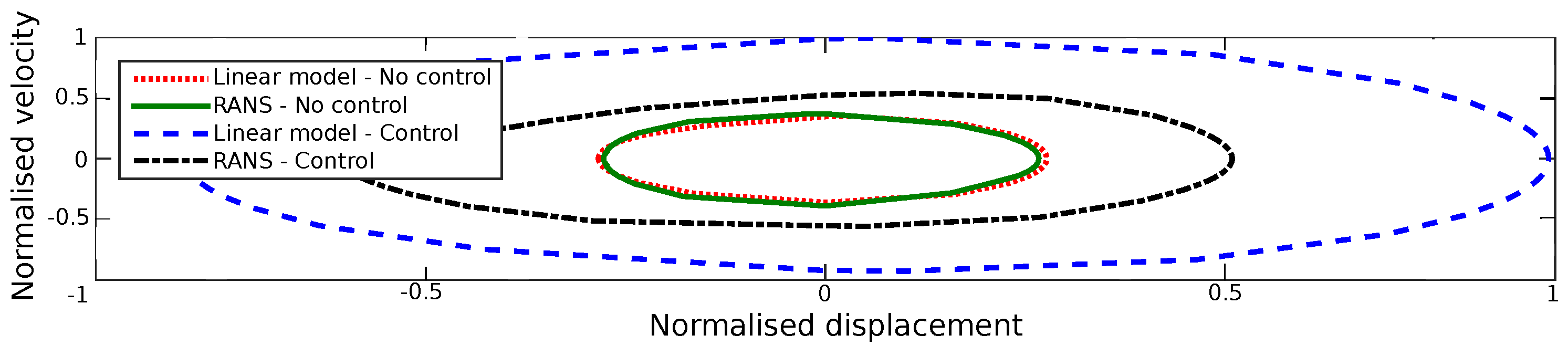
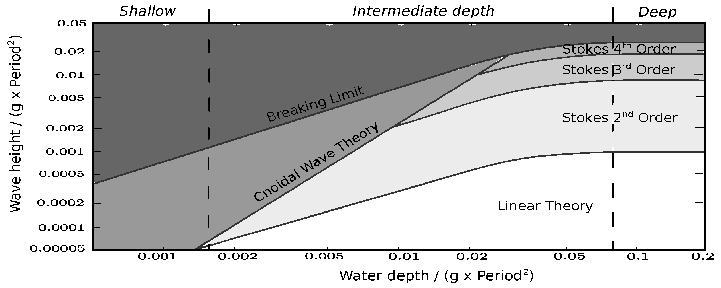
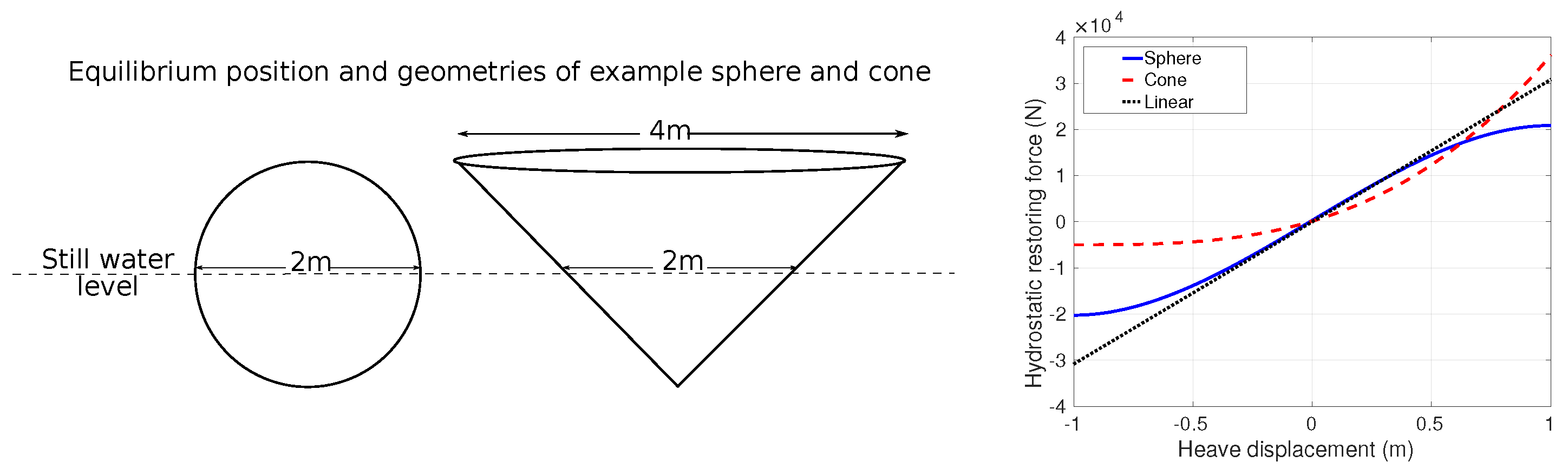
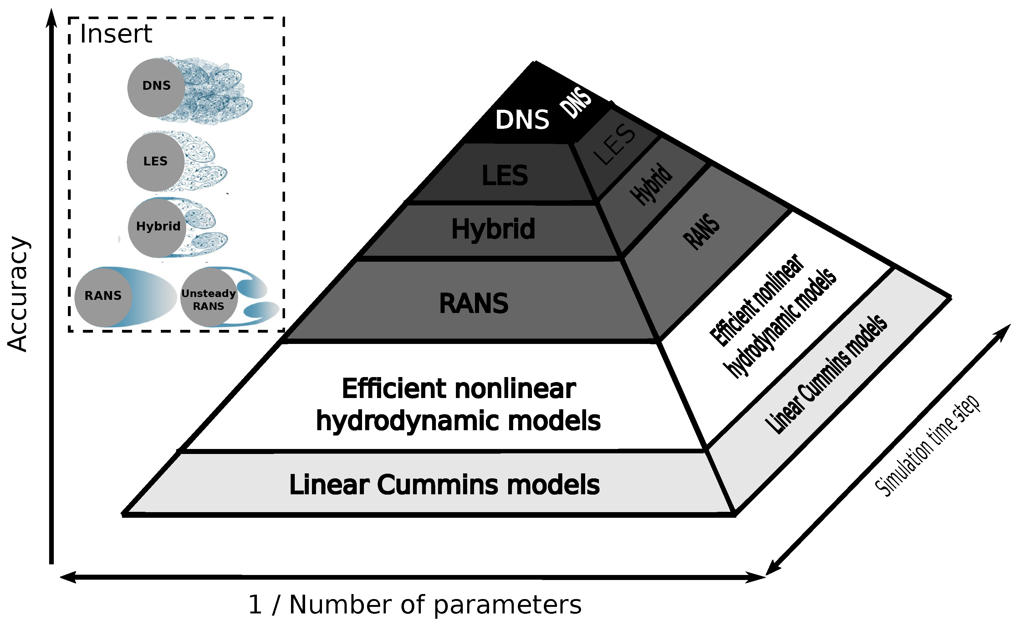
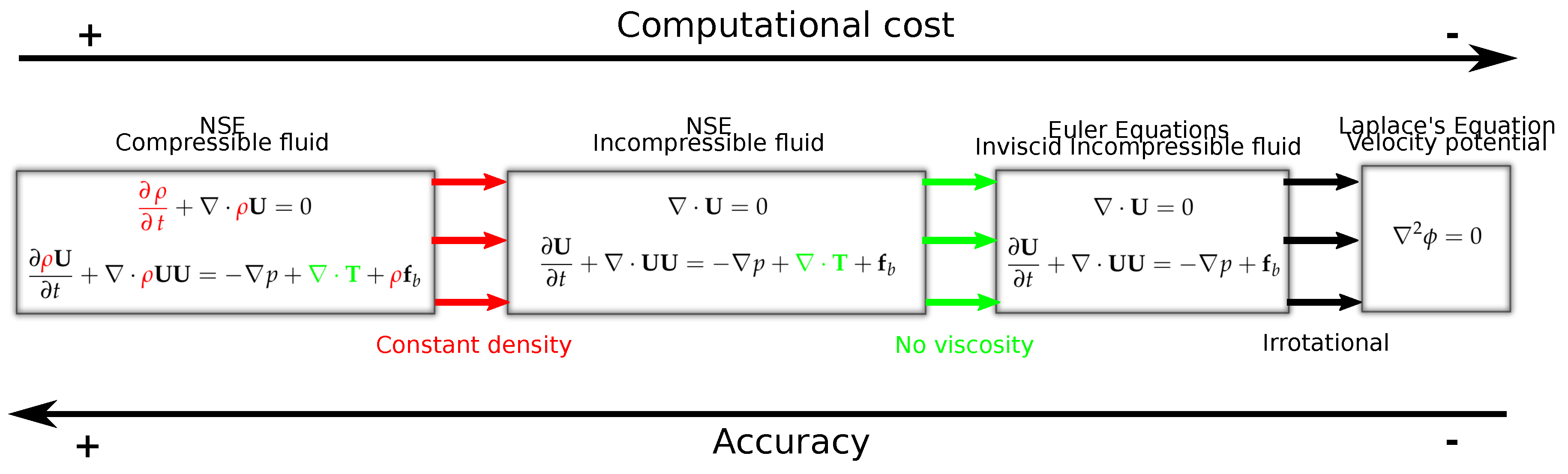
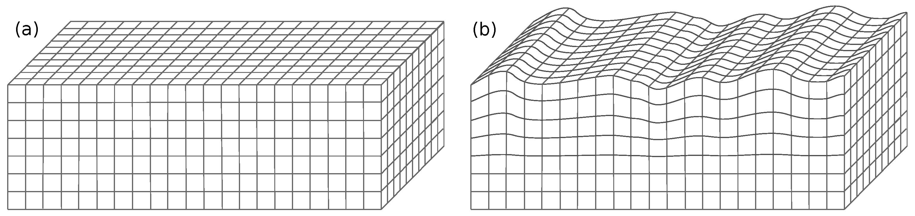
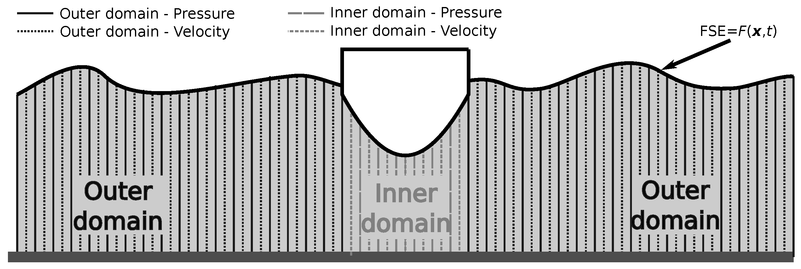
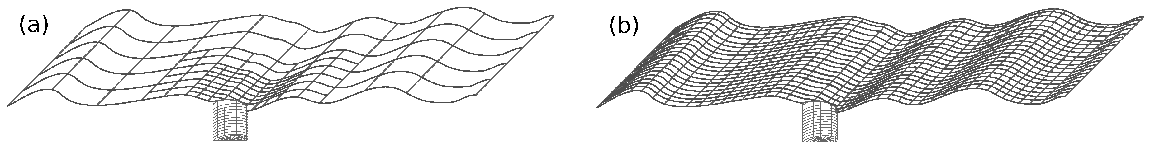
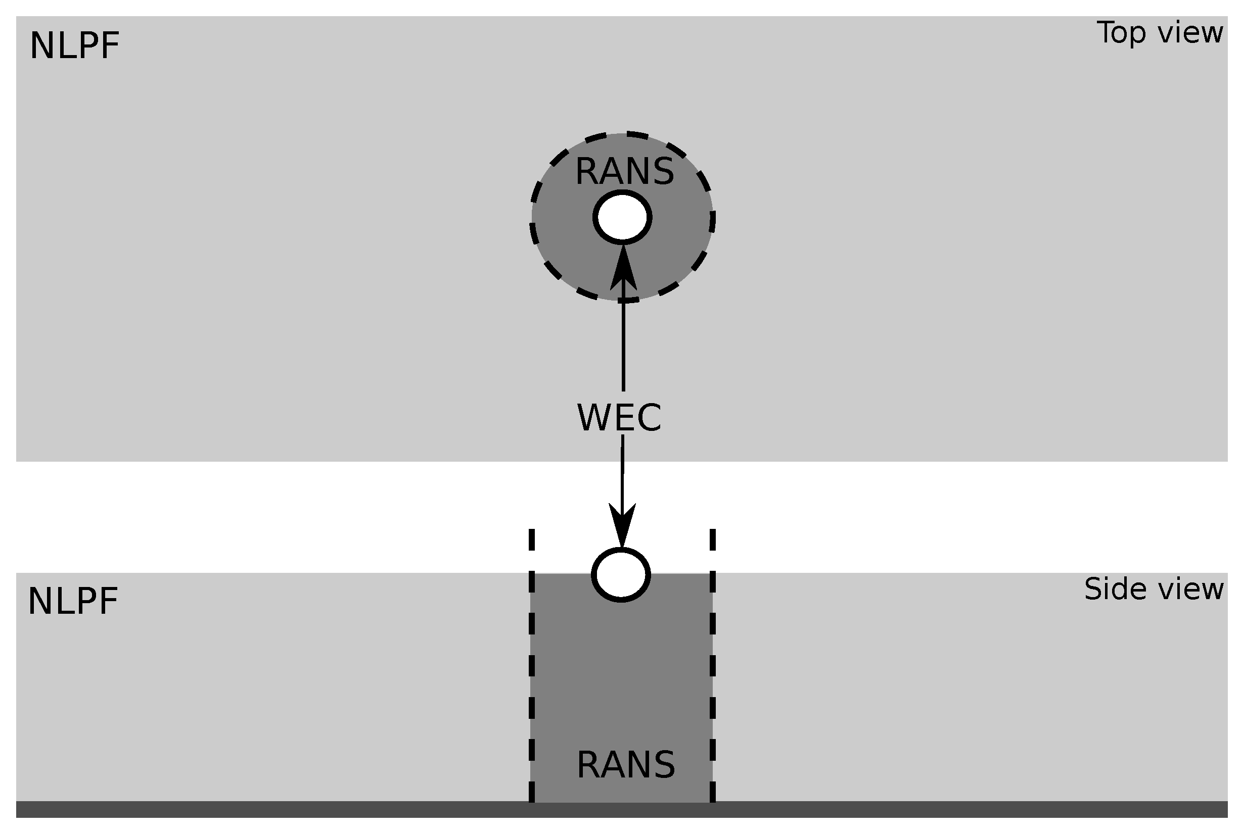
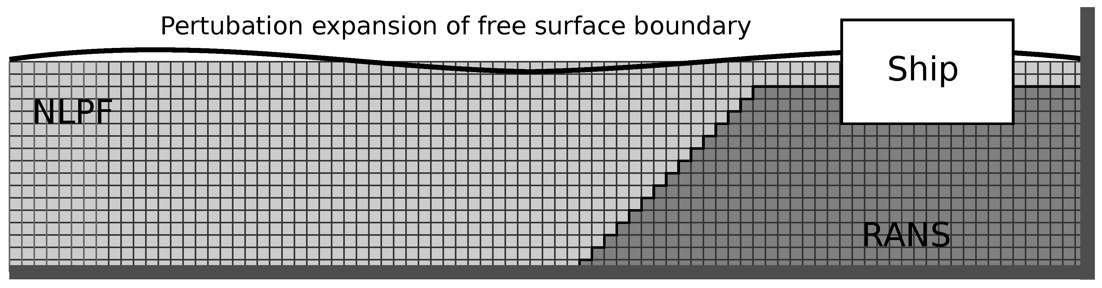
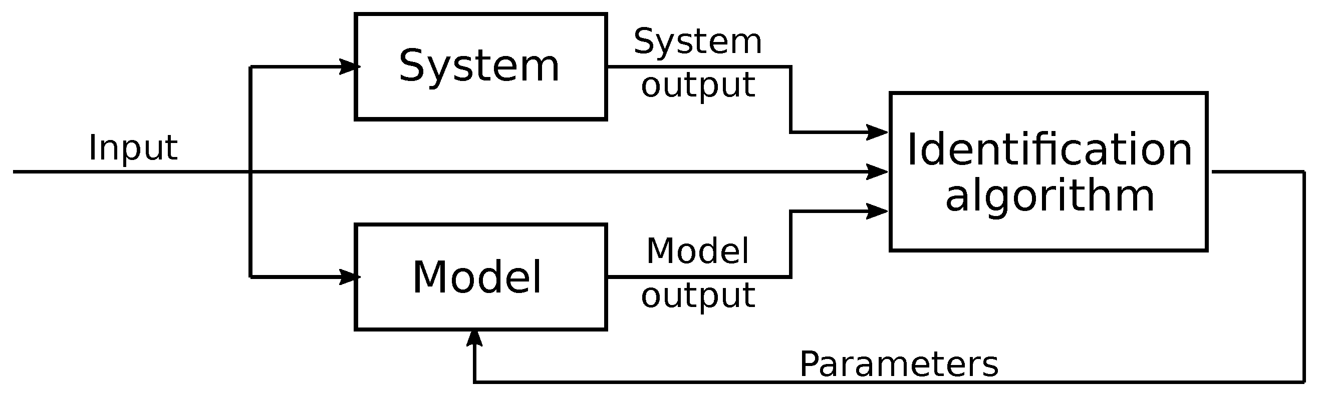
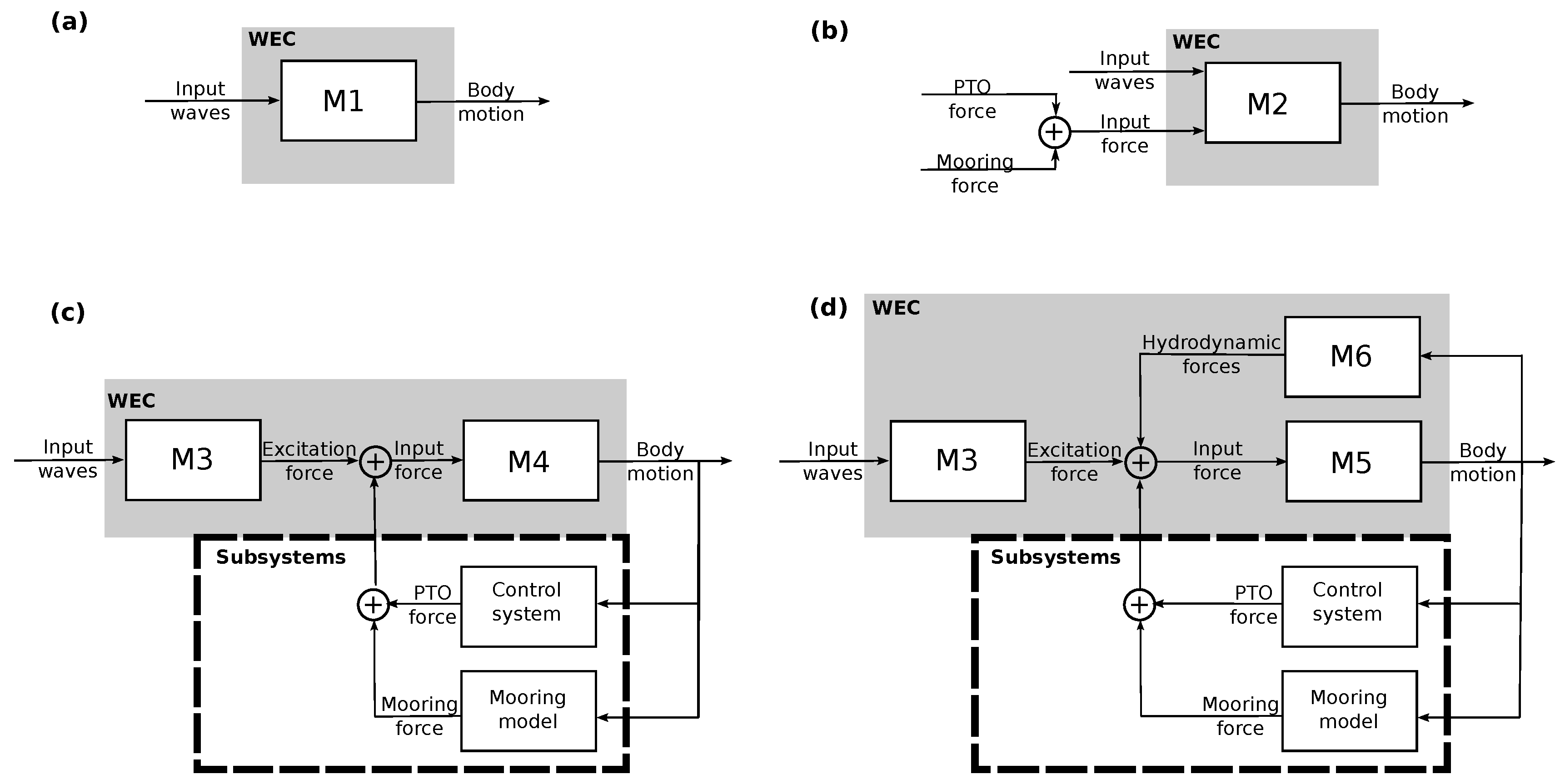
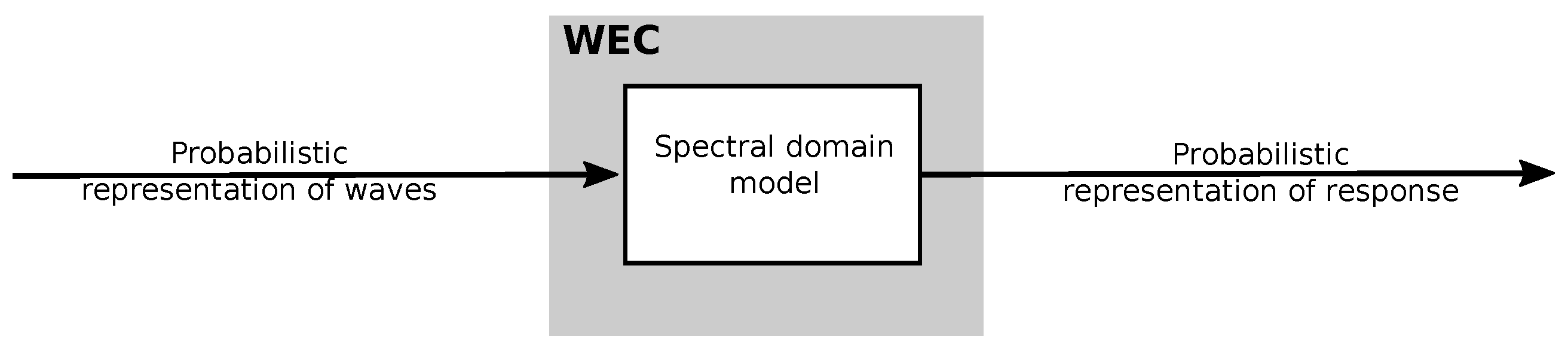
Figure 1. (a) The Technology Readiness Level (TRL)—Technology Performance Level (TPL) matrix: wave energy converter (WEC) technology value map. (b) The TRL-TPL matrix, highlighting two different development trajectories to commercial viability: Path A represents the Performance before Readiness approach, and Path B is a more expensive trajectory (adapated from Weber et al. [1]).
Jmse 08 00035 g001
Figure 2. Comparison of the displacement-velocity operational space for a heavy point absorber (HPA) in a JONSWAP sea spectrum, with and without an energy maximizing controller, predicted using a linear Cummins equation model and a Reynolds averaged Navier–Stokes (RANS) simulation, from the case study presented in Davidson et al. [26].
Jmse 08 00035 g002
Figure 3. The validity limits of different wave theories dependent on the water depth, the wave height and the wave period. The region in which linear theory is valid is shown in white (Adapted from [31]).
Jmse 08 00035 g003
Figure 4. Hydrostatic restoring force for a sphere and a cone.
Jmse 08 00035 g004
Figure 5. Schematic comparison of the accuracy versus computational requirements for solving the NSE. The more parameters and the smaller the timestep, thus the smaller the cross-sectional area of the pyramid at a given height, the greater the computational requirements. Here the vertical scale is likely logarithmic, the horizontal scales exponential and the cut-off positions between methods are not exact (Image inspired from [49,50]). The white region, “Efficient nonlinear hydrodynamic models,” represents the focus of the scoping study. (Insert: Example simulation resolution from the different methods, for airflow past a dimpled sphere, adapted from [51]).
Jmse 08 00035 g005
Figure 6. Hierarchy of simplifying assumptions applied to the NSE, yielding lower accuracy and more computationally efficient equations for hydrodynamic analysis (adapted from [63]).
Jmse 08 00035 g006
Figure 7. Schematic of the finite volume discretization and the one fluid/two-phase (air and water) modeling for the Euler equations.
Jmse 08 00035 g007
Figure 8. Schematic of the mixed Eulerian–Lagrangian (MEL) scheme. (a) Equilibrium position with no waves and (b) dynamic motion of the mesh to capture time-varying free surface.
Jmse 08 00035 g008
Figure 9. Schematic of unified Boussinesq approach in Jiang and Henn [155], showing the outer and inner domains, the single cell in the vertical dimension discretization and the staggered finite difference method (FDM), where velocity and pressure control volumes do not coincide.
Jmse 08 00035 g009
Figure 10. Schematic of the computational domains for (a) the weak scatter and (b) the FNPF methods.
Jmse 08 00035 g010
Figure 11. Schematic of domain decomposition using nonlinear potential flow (NLPF) in the far-field and Reynolds averaged Navier–Stokes (RANS) in the near field.
Jmse 08 00035 g011
Figure 12. Domain decomposition to capture flow separation around a ship in [272].
Jmse 08 00035 g012
Figure 13. Schematic of the system identification (SID) approach to obtain computationally efficient parametric models. The real system to be modeled generates the input and output data which are utilized by the identification algorithm to estimate the parameters of the model.
Jmse 08 00035 g013
Figure 14. Schematic of the various inputs and outputs to the models. (a) Input waves only. (b) Input waves and subsystem forces. (c,d) Input waves with modelling of the subsystems.
Jmse 08 00035 g014
Figure 15. General structure of a spectral domain model (reproduced from [322]).
Jmse 08 00035 g015
Table 1. Review of publications utilizing the Euler equations for wave energy converter (WEC) simulation.
Ref.SoftwareWEC TypeAnalysis
[64]AMAZON-3DManchester BobberExtreme wave loadings
[65]AMAZON-3DManchester BobberSlamming
[66]AMAZON-3DManchester BobberSurvivability design scenarios
[67]OpenFOAMWave-DragonOver-topping
[34]OpenFOAMHPAInvestigation of parametric resonance
[47]OpenFOAMHPAInvestigation of scale effects
Table 2. Review of publications utilizing fully nonlinear potential flow (FNPF) for WEC simulation.
Ref.MethodWEC TypeAnalysis
[69]Cauchy’s EqnSalter’s Duck (2D)Capsizing in extreme waves
[70]Cauchy’s EqnSubmerged wave lensFocusing of wave energy
[72]BEMOWC (2D)Geometry analysis
[73]BEMLand-based OWC (2D)Validation against RANS and experiments
[74]HOBEMBristol Cylinder (2D)Proof of modeling concept
[75]BEMFloating OWC (2D)Using the acceleration potential method
[76]BEMFloating OWC (2D)Including viscosity to NLPF model
[77]BEMFloating OWC (2D)Evaluating sharp versus round corner geometry
[29]HOBEMFixed OWC (2D)Investigating hydrodynamic performance
[78]HOBEMSubmerged cylinder (2D)Proof of modeling concept
[79]BEMRolling-cams (2D)Including viscosity to NLPF model
[80]HOBEMBristol Cylinder (2D)Validation against experiments
[81]BEMFixed OWCInvestigation of stepped-bottom OWC
[82]BEMHPA (Cylinder)Effect of wave steepness
[43]HOBEMFixed OWC (2D)Including viscosity to NLPF model
[83]BEMOSC (2D)Hydrodynamic performance for large motion
[84]HOBEMOSCPerformance in waves and currents
[85,86]BEMHPA (Cylinder)Latching control/Wave-body-PTO interaction
Table 3. Review of publications utilizing depth-averaged equations for WEC simulation.
Ref.MethodWEC TypeAnalysis
[143]Boussinesq (SEM)HPAComparison against linear and RANS models
[144,145,146]Boussinesq (SEM)HPA (2D)Verification and validation of model
[147,148]Congested shallow waterHPA (2D)Verification and validation of model
[149,150]
Non-hydrostatic flowSubmerged PASimulate interactions between nonlinear wave
field and WEC over coastal scale regions
[151]Non-hydrostatic flowSubmerged PAParametric instability
[152]Non-hydrostatic flowSubmerged PAGeotechnical stability of the moorings
Table 4. Review of publications utilizing weakly nonlinear models for WEC simulation.
Ref.MethodWEC TypeAnalysis
[163]PerturbationOWCNonlinear free surface effects
[164]2nd Order PFTight moored piston-like WECPerformance of 2-body system with moonpool
[165]WSAPA with pendulum PTOPowering small scale data buoys
[166]2nd Order PF2 × HPA (Hemisphere)Array interaction
[167]2nd Order PFFixed cylindrical OWCEffect of weakly nonlinear waves on efficiency
[168]WSAHPA (Sphere)Comparison against linear and NLFK models
[169]2nd Order PF4 × HPA (Cylinder)Trapped modes in arrays
[170]WSACETOCoupling with multi-body mechanical solver
[171]WSAWavestarComparison against linear and NLFK models
[172]WSACETO and WaveRollerComparison against linear models
[173]2nd Order PFOSC arraySub-harmonic and higher-order effects
[174]2nd Order PFCurved gate (2D)Nonlinear effects of the curved surface
[175]2nd Order PFCurved OSC arrayNonlinear effects of the curved surface
[176,177]3rd Order PFCurved gate arrayNonlinear effects of the curved surface
Table 5. Review of publications utilizing partially nonlinear models for WEC simulation (Note: NLFK method not collated because of the large number of publications).
Ref.WEC TypeAnalysis
[188]OSCImproved model accuracy for large pitch angles
[189]OSCImproved model accuracy for large pitch angles
[190]Submerged HPADemonstration of method
[191]Reconfigurable OSCModeling change in hydrodynamics for moving control surfaces
[35]HPAModeling the occurrence of parametric pitch resonance
[192]OSCImproved model accuracy for large pitch angles
Table 6. Review of publications utilizing Domain Decomposition for WEC simulation.
Ref.MethodWEC TypeAnalysis
[228,229]FD to TD PFPico OWCEfficient TD simulations
[230]Wave model to PFArray (HPA)Wave interactions with WEC array
[231]Wave model to RANSOSCModeling real bathymetry
[232]PF to I.RANS to C.RANSOSCSlamming loads
[233,234]Wave model to PFArrayMultiple WECs in variable bathymetry
[235,236]Wave model to PFArray (OSC)Wake effects in arrays
[237,238]Wave model to PFMultiple Arrays (HPAs)Impact of WEC array separation distance
[239]Wave model to PFArrays (HPAs and OSCs)Comparison of far-field effects
[240,241]Wave model to PFArray (HPAs)Validation of model
[242,243,244]NLPF to SPHHPAProof of concept
[245]NLPF to SPHOWCDemonstration of method
[246]NLPF to RANSHPABlind comparison test [247]
Table 7. Review of publications utilizing system ID for WEC simulation, detailing the parameterization employed, the data source used, the type of WEC investigated, and the analysis performed.
Ref.ParameterizationDataWEC TypeAnalysis
[300]
[193]
State-spaceRANSHPAID of amplitude dependant equivalent
linear models
[301]State-spaceRANSOWCHeave motion in OWC chamber
[204]Cubic polynomialPWTWavestarNonlinear restoring force
[302]
[303]
Hammerstein-
Weiner Volterra
Thermo-
dynamics
OWCAir pressure fluctuations inside
OWC chamber
[304]NARXRANSHPANonlinear hydrostatic restoring force
[305]ANNRANSHPAOptimization of input/out data for SID
[306]Volterra theoryPWTOWSCID of accurate models from PWT data
[307]ARX, Hammerstein, KGPRANSHPANonlinear excitation force
[308]ARX, KGP, ANNRANSHPASID of nonlinear discrete-time models
[309]Grey- and black-boxPWTHPAInvestigation of SID techniques
[310]
[221]
Pseudo-spectralRANSHPAOnline ID of time-varying equivalent
linear models for adaptive control
[311]Multi regression modelCFD + PWTOWCEmpirical model design tool
[312]ARX, KGPPWTWavestarNonlinear model ID from PWT data
Table 8. Review of publications utilizing probabilistic methods for WEC simulation.
Ref.MethodWEC TypeAnalysis
[318]FDOWCOptimization of turbine size and rotational speed
[220]SDOSWCModeling vortex shedding and large amplitude effects
[321]FDHPAGeometry, mass distribution, and mooring design optimization
[323]SDHPA (Array)Modeling arrays and Coulomb friction
[324]SDOWCValidation of model against tank data
[325]SDOSWCAccommodate nonlinear WEC dynamics in an optimal controller
[326]SDOSWCInvestigation of controllable surfaces
[319]FDSpar buoy OWCStatistical values of device dynamics and power output for an array
[327]SDHPA (Sphere)Modeling nonlinear hydrostatic stiffness
[328]SDSubmerged PAInclude nonlinear viscous drag and compare with other methods
[329]PCHPAPredicting long term extreme loads
[330]PCHPAUncertainty quantification
[331,332]SDHPA/OWCStatistical linearization of nonlinearities
[320]FDSpar buoy OWCDesign optimization
Table 9. Review of publications utilizing NLFD models for WEC simulation.
Ref.WEC TypeAnalysis
[340]OSC + HPA (Sphere)Demonstration of modeling approach
[341]HPA (Sphere)Model’s ability to handle different nonlinearities
[343]OSCComputationally efficient control
[346]OSC + HPA (Sphere)Effect of spectral shape of wave spectrum on power output estimates
[342]ISWECComparison against MDoF time-domain models
[344]Ocean GrazerPTO system performance of a single device
[345]Ocean GrazerPTO system performance for full array
Table 10. Requirements of the different end uses of a WEC simulation tool.
ApplicationTime-SpanSpatial DomainHydrodynamic Resolution
Section 6.1.1 WEC operationVast—interested in characterizing and optimizing the device performance across all sea states at a given locationSmall—local effects onlyHigh—accurate modeling required for assessment of device performance
Section 6.1.2 WEC survivalSmall—interested in the subset of all sea states, and wave series within those sea states, which give rise to maximum loadsSmall—local effects onlyVery high—must be able to capture the very nonlinear waves and WSI associated with extreme wave conditions
Section 6.1.3 WEC farmsMedium—time averaged interactions between the wave farm and the environmentVery large—must simulate the entire domain of the wave farmMedium—interested in the average effects of the interactions between fully designed WECs in arrays/farms
Table 11. Review of publications utilizing open-source software.
SoftwareReferencesSoftwareReferences
OpenFOAM[9,26,27,34,35,45,46,47,54,56,57,61,67,125,139,143,146,159,190,193,217,221,232,246,247,258,259,260,261,262,265,266,267,268,269,270,272,273,274,275,277,284,300,301,304,305,307,308,310,314,353,364]SPHysics[242,243,244,245]
Nemoh[172,179,189,190,192,205,206,216,235,236,237,238,239,240,241,249,250,344,346]Gmsh[123,180]
OceanWave3D[129,131,132,134,242,243,244,245,250,266,268]Grid2Grid[264,265]
WEC-Sim[192,195,330,358,359]ExaFMM[91]
SWASH[149,150,151,152,162]Palabos[53]
HOS Ocean/NWT[100,103,132,201]Nektar++[120]
Table 12. Comparison of the reviewed efficient nonlinear hydrodynamic modeling methods.
StrengthsLimitations
Euler Equations• Can simulate wave breaking, green water etc. • Simulates both air and water phases • Can include drag and vortex effects • Implementable in CFD solver frameworks e.g., OpenFOAM• Computationally expensive • Waves must be solved and propagated to WEC location
FNPF• Large amplitude waves and body motions permitted • Currently the focus of much research and development • Flexible/deformable bodies can be easily handled by FEM/SEM • Well suited for use in domain decomposition with RANS• Computationally feasible with adequate hardware • Waves must be solved and propagated to WEC location • Design of efficient and flexible methods to handle both the nonlinear wave propagation and wave-body interactions is non-trivial, as FNPF NWTs have traditionally been designed to focus on one or the other.
Shallow water• Efficiency is gained by eliminating/reducing the vertical dimension and by representing the free-surface as a single-valued function • Valid in the nearshore• While this method has been shown to work effectively for floating bodies, it is unclear if this could be applicable to submerged bodies • Loses validity in the deep water • Waves must be solved and propagated to WEC location
Weak scatterer• Large body motions • Nonlinear steep incident waves • Incident wave does not need to be solved and propagated • Mesh only needs to be refined close to the WEC and large cells can be used elsewhere• Valid for small perturbed waves • Computational expense in updating the computational domain at each time step, like FNPF
WNPF• FD possible • Efficient time-domain simulations since the hydrodynamic coefficient matrices are the same for every time-step, thus only need to be set-up and inverted once. • Incident wave does not need to be solved and propagated• Although an improvement upon LPF, this method still contains limitations on the wave steepness and amplitude of body motion
Time-varying parameters• Computationally efficient • Can precompute the required hydrodynamic coefficients offline beforehand and use look-up tables/interpolation during simulation • Can input wave signal directly, rather than generated at boundary and propagated to the WEC• Body nonlinear only, with linear assumptions still applied on the input waves • Might only be suitable for NLFK forces, since implementation of time-varying linear models for radiation and diffraction forces is unclear due to memory effects and convolution integrals in time.
NLFK• Computationally efficient • Can consider nonlinear/steep waves • Can input wave signal directly, rather than generated at boundary and propagated to the WEC• Only useful for WEC geometries for which the NLFK forces are significant • Not applicable for fully submerged devices • Linear wave radiation and diffraction forces
Domain decomposition• Can provide high fidelity WSI equivalent to RANS and better wave propagation modeling, for less computational effort than RANS • Can be used for extreme and survival conditions • Can be used for large spatial scales considering WEC arrays and wave farms• Computationally expensive • Two-way coupling methods not yet mature/widely demonstrated
Parametric models identified from data• Computationally efficient time-domain simulations with fidelity equivalent to the data used to identify the model • Can input wave signal directly, rather than generated at boundary and propagated to the WEC• Requires high fidelity training data set spanning the frequency and amplitude ranges • Models may not accurately extrapolate to input conditions outside the range which they were trained upon
Spectral Domain• Extremely fast calculation of statistical values, such as mean annual power output etc.• No temporal responses • Unable to model monochromatic waves • Only valid for Gaussian inputs • The accuracy of the SD model decreases with the deviation from a Gaussian response, therefore unsuited to some nonlinear forces, such as abrupt end-stop collisions, latching control etc.
Polynomial chaos• Can test wide ranges of design variables, without simplifying the physics involved.• Restricted to relatively low number of dimensions in the parameter space (curse of dimensionality) • Smoothness restrictions on the quantity of interest
NLFD• Can produce time-domain results an order of magnitude faster than traditional Cummins equation methods • Can input wave signal directly, rather than generated at boundary and propagated to the WEC• Linear assumption on input waves • WEC outputs must remain smooth, therefore cannot handle abrupt end-stop collisions, latching control etc • Periodic steady-state responses only

