Abstract
A new approach based on the multigene genetic-programming (MGGP) technique is proposed to predict initial dilution of vertical buoyant jets subjected to lateral confinement. The models are trained and tested using experimental data, and the good matches demonstrate the generalization and predictive capabilities of the evolved MGGP-based models. The best Pareto-optimal MGGP-based model is also compared with the model evolved using a single-gene genetic-programming (SGGP) algorithm and an existing regression-based empirical equation. The comparisons reveal the superiority of the MGGP-based model. This study confirms that the MGGP technique is promising in evolving an explicit, accurate, and compact model, and the developed models can be employed to estimate effectively and efficiently the dilution properties of a laterally confined vertical buoyant jet.
1. Introduction
Liquid wastes from municipal and desalination activities in coastal areas are often discharged into the receiving water body in the form of wastewater jets [1,2,3,4,5,6]. Such jets are referred to as buoyant jets if their densities S.are lower than that of the ambient water. Wastewater discharges can significantly jeopardize the marine environment and ecology, so it is important to understand better the dilution and mixing properties of buoyant jets for an efficient design of the outfall systems and accurate evaluation of the environmental and ecological impacts.
After discharge into the receiving water body, an effluent jet spreads and mixes with the ambient water because of the jet advective and diffusive transport processes and the shear stresses at the interface between the jet and ambient water. Different from a turbulent plume, which is driven entirely by buoyancy effects, a buoyant jet is driven by both momentum and buoyancy effects, and thus the well-established turbulent plume theory [7,8,9] cannot be utilized for wastewater jets. Depending on the dynamic interactions with neighboring boundaries, a buoyant jet can be classified as either a free or confined buoyant jet. When a jet is far from any boundary, the jet can freely spread in and mix with the ambient water. Thus, the rapid jet spreading and ambient water entrainment can effectively dilute the wastewater effluent. However, jets are often subjected to the effects of boundaries in some practical applications [10,11,12], such as the jets issued from outfall systems that are in dredged trenches or those with protective riser tubes (Figure 1). In such applications, the confinement could suppress the jet spread and restrict the intrusion of the ambient water into the jet, and thus affects the jet dilution. Such effects make the dilution and mixing processes more complicated and require further investigation.
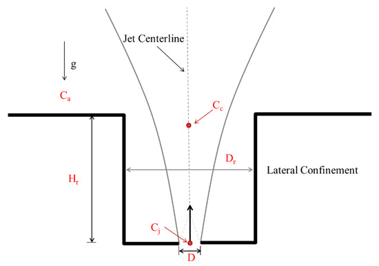
Figure 1.
Sketch of a laterally confined vertical buoyant jet.
Confined jets have been extensively studied in the past several decades due to both academic and practical interests. Experimental works on confined jets have involved the measurements of flow and mixing properties of a gas jet injected from an orifice into the gas flow in a rectangular-sectioned duct [13], PIV (particle image velocimetry) measurements of the turbulence distribution in the bulk free region of a vertically injected confined jet [14], LIF (laser-induced fluorescence) measurements of concentration distribution of a vertical buoyant jet subjected to lateral confinement [10], PIV measurements of the velocity field of a horizontal jet subjected to vertical confinement [15], and PIV and planar LIF measurements of the flow and mixing parameters of multi-lateral jets discharged into a round pipe flow [16]. A limited number of previous modeling works also involved the development of theoretical or numerical models for confined jets. Jirka [17] presented an integral model that can model the jet mixing properties with both the lateral and vertical confinement being considered. El-Amin et al. [18] conducted numerical modeling of the flow and temperature fields of a two-dimensional buoyant confined jet injected vertically into a cylindrical tank. More recently, Yan and Mohammadian [19] simulated a laterally confined vertical buoyant jet as a three-dimensional phenomenon by solving the full Navier-Stokes equations. These experimental and numerical studies have provided comprehensive and reliable data sets for a better understanding of confined jets and promising tools for estimating the flow and mixing properties of confined jets. However, such approaches are typically too expensive or time-consuming for practical applications, and thus it is very beneficial to propose a new tool that is more efficient.
Over recent years, artificial intelligence (AI) techniques have been widely introduced to solve water and marine engineering problems. For example, Kisi et al. [20] presented the earliest application of the adaptive neuro fuzzy inference system (ANFIS) to estimate sediment in rivers; Hipni et al. [21] employed the support vector machine (SVM) and ANFIS to forecast the daily dam water levels, Rezaei et al. [22,23] proposed the fuzzy Multi-Objective Particle Swarm Optimization (f-MOPSO) algorithm for conjunctive water use management, and Bashiri et al. [24] used the harmony search algorithm and artificial neural networks (ANN) to predict local scour depth downstream of sluice gates. Recently, Moroni et al. [25] reviewed the literature regarding an environmental decision support system for oil spill management, and stated that the provision of support services is generally based on AI paradigms. Compared with some other AI techniques, such as ANN and ANFIS, genetic programming (GP) algorithm has the advantage of being able to automatically evolve an explicit mathematical model. One of the most recent variants of GP is the multigene genetic-programming (MGGP) technique [26,27] An MGGP model is a combination of multiple genes, and each gene is a traditional GP gene. It has become very popular in the past several years. Garg et al. [28] developed some MGGP-based soil water retention curve models for three different soils. These models describe the water content as functions of net stress and suction, and the results showed that the predictions made by these MGGP-based models matched the measurements very well. Kaydani et al. [29] applied several AI techniques, including ANN, ANFIS, traditional GP, and MGGP, to predict the permeability in a heterogeneous oil reservoir. Their study demonstrated that the MGGP technique was more advantageous than the other AI techniques in permeability estimation in terms of providing a relatively compact model and avoiding structural dependency. More recently, Safari and Mehr [27] developed a Pareto-optimal model using MGGP to model particle Froude numbers in large sewers. Their research outcome has demonstrated that the proposed MGGP model can provide more accurate predictions than the existing conventional regression models. These studies encouraged the application of AI techniques to water-related problems.
Despite the generalization and predictive capabilities of AI techniques, very few applications of AI techniques have been employed in predicting the dilution properties of wastewater effluents. To the best of the authors’ knowledge, an MGGP-based model for initial dilution of laterally confined vertical buoyant jets has not been reported in the literature. Therefore, the present paper develops MGGP-based models that can predict the jet concentration as functions of the jet densimetric Froude number, Fr, the confinement index, β, and the location of the cross section, Z/D. Three of the Pareto-optimal models are compared with experimental data for both the training and testing periods, and the best model is determined with both the performance and simplicity considered. The best MGGP-based model is also compared with a single-gene genetic-programming (SGGP)-based model and an existing regression-based empirical model, and the results demonstrated the superiority of the MGGP-based model.
2. Methods
2.1. Analysis of a Laterally Confined Vertical Buoyant Jet
The initial dilution of a free buoyant wastewater jet is primarily affected by the discharge volume flux, Q, kinematic momentum flux, M, and buoyancy flux, B, defined as Q = (π/4)D2uj, M = ujQ, and B = g’Q, where D is the port diameter, uj is the initial jet velocity, and g’ is the modified gravitational acceleration. Following a dimensional analysis, characteristic variables can be typically defined as functions of D and the densimetric Froude number, Fr [1,10,19,30,31]. Fr characterizes the relative importance of inertia over buoyancy as:
with
where g is the gravitational acceleration, ρa is the density of ambient water, and ρj is the initial jet density.
For a vertical buoyant jet subjected to lateral confinement (Figure 1), the properties of initial dilution are quite different from those of a free buoyant jet, primarily because the existence of lateral confinement suppresses the jet spreading and the intrusion of ambient water into the jet. Therefore, the effect of lateral confinement should also be considered in the prediction of the initial dilution. Dilution properties can be represented by jet concentration, and the dimensionless form can be expressed as (C − Ca)/(Cj − Ca), where C is the concentration at a point, Ca is the concentration of the ambient water, and Cj is the initial jet concentration. Because the dilution properties are mainly affected by Fr and the confinement, the dimensionless concentration can be expressed as a function of the dimensionless confinement diameter, Dr/D, dimensionless confinement height, Hr/D, and dimensionless cross section, Z/D, as:
where Z is the vertical displacement of a cross section, and D is the port diameter.
The cross-sectional concentrations of a free buoyant jet or a laterally confined vertical buoyant jet at different representative cross sections can be fitted to a Gaussian profile as [19,32]:
where Cc is the centerline concentration at a cross section, r is the radial distance of a point from the centerline, and bgc is the half concentration width. Therefore, the concentration field can be easily estimated if Cc is known, and thus the key parameter characterizing the dilution properties is the jet centerline concentration. In order words, developing an MGGP model for Cc is significant because estimating Cc from the flow and geometrical variables is quite challenging, but in this case developing an MGGP model for the concentration distribution is not necessary because it can be efficiently estimated using Equation (4) after Cc is calculated. Therefore, the present study selected the jet centerline concentration as the output variable.
The geometrical parameters of lateral confinement, Dr/D and Hr/D, can be combined, and the combined parameter is referred to as the confinement index, β, which is defined by β = (Hr/D)/[(Dr/D)−1]. Therefore, the dimensionless jet centerline concentration can be expressed as:
Therefore, a major objective of this paper is to develop an MGGP-based model for the dimensionless jet centerline concentration as function of Fr, β and Z/D.
2.2. Experimental Data Sets
Lee and Lee [10] conducted extensive experiments on the initial dilution of laterally confined buoyant jets, which have provided comprehensive data sets. The majority of the work was conducted in a 1 × 1 × 0.5 m water tank with the water depth being kept at about 0.45 m. Heated water was vertically discharged into the tank from the bottom of the tank through a nozzle. A riser tube was utilized for lateral confinement. The concentration field for each case was measured using a laser-induced fluorescence (LIF) technique. A wide range of jet diameter, riser diameter, riser height, jet temperature, ambient temperature, and jet velocity were investigated, with Fr ranging from 3.0 to 18.7 and β ranging from 1.47 to 12.3. A total of 442 experimental data points derived from 58 tests were utilized in the present study, with 80% of them being employed for model training and the remaining 20% for model testing. The splitting of data sets was performed randomly with the assistance of MATLAB’s random-permutation function.
2.3. The MGGP Method
MGGP is one of the most recent variants of GP, which is a popular evolutionary technique that has been extensively applied to developing data-driven nonlinear models. As a branch of GP techniques, MGGP can automatically evolve an explicit model using training data sets without the need for defining the model structure in advance [33]. This can not only facilitate the development of a mathematical model but can also avoid errors due to some subjective judgments, especially judgments regarding the model structure. Compared with the standard GP technique, MGGP primarily has two clear advantages because it allows for multiple genes: first, each gene in an MGGP model is a traditional GP gene, so MGGP can be more accurate; second, each MGGP gene only needs to contain a few tree depths, so the orders of the nonlinear terms in each gene are lower, and thus an MGGP model is usually more compact.
MGGP develops a mathematical model in an evolutionary process. An example of the evolutionary process is illustrated in Figure 2. At the beginning of the MGGP algorithm, multiple genes are randomly generated. The mathematical expressions of Gene 1 and Gene 2 in the first generation shown in Figure 2 are
and
where x1 and x2 are the input variables.
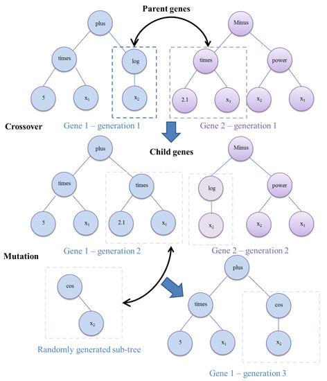
Figure 2.
Example of the tree structure and evolving processes of an MGGP chromosome.
The model in the initial generation typically has a low level of fitness, so more generations are created with the process of reproduction, crossover, and mutation to improve the model performance. In a crossover process, sub-trees in different genes are interchanged. For the example in Figure 2, the sub-trees log(x2) and 2.1x1 of the parent genes are exchanged, and child genes (the second generation) are formed, which can be expressed as:
and
In a mutation process, a sub-tree within a gene is replaced by a new element. For the example in Figure 2, the sub-tree 2.1x1 is replaced by cos(x2), forming a new form of Gene 1 (in the third generation) as:
The multiple genes are linearly combined together to form a complete MGGP model. For the example in Figure 2, the MGGP model is:
where α1 and α2 are the weights of Genes 1 and 2, respectively; and γ is the bias term. These weights and the bias term are determined using an ordinary least-squared method.
2.4. MGGP Modeling Setup
To develop an MGGP model for the initial dilution of a laterally confined vertical buoyant jet, the dimensionless jet centerline concentration was set to be the output variable and the dimensionless parameters Fr, β and Z/D were used as input variables. The MGGP evolutionary processes were conducted using the toolbox GPTIPS2 [26], which is an open-source code set that can be modified and executed in the standard MATLAB environment. The population size and maximum generations were set to be 250 and 150, respectively. The tournament size and probability of Pareto tournament were set as 20 and 0.3, respectively. To ensure model simplicity, the maximum tree depth and maximum genes were both set to be 5. The maximum total nodes were set as infinite. The elite fraction, crossover probability, and mutation probabilities were set as 0.3, 0.84, and 0.14, respectively. The function set includes ‘times’, ‘minus’, ‘plus’, ‘rdivide’, ‘square’, ‘sin’, ‘cos’, ‘exp’, ‘mult3’, ‘add3’, ‘sqrt’, ‘cube’, ‘power’, ‘negexp’, ‘neg’, ‘abs’,’ log’. These configurations were determined in preparatory studies to ensure model simplicity, convergence efficiency, and model accuracy. The detailed procedures are summarized as follows: (1) the available experimental data points were randomly divided into two groups: training and remaining; (2) MGGP models were trained using the process and configurations described earlier in this paper; (3) the developed models were employed to compute the dimensionless jet centerline concentration as a function of Fr, β and Z/D for the training dataset, and the optimal models were selected; and (4) the selected models were utilized to carry out additional computations for the testing dataset, and their performances were evaluated. An SGGP modeling was also performed, and the only difference in the SGGP parameter setup from that in the MGGP modeling was that the maximum number of genes was set to be 1.
3. Results and Discussion
3.1. Pareto-Optimal MGGP Models
Figure 3a illustrates the performance-complexity trade-off of the evolved MGGP models for dimensionless jet centerline concentration. Determining the best model needs to consider two conflicting objectives simultaneously: accuracy and simplicity. Therefore, the Pareto optimization method was utilized. The green circles in Figure 3a denote the non-dominated solutions (i.e., there exists no solution that is more accurate and less complex at the same time) and the corresponding evolved MGGP models are referred to as the Pareto-optimal models [27]. These models are regarded as optimal because a solution cannot improve the model performance without increasing the complexity, and vice versa.
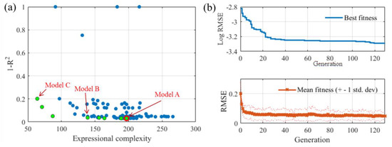
Figure 3.
The Pareto front plot of the evolved MGGP-based models and convergence of the solutions: (a) Pareto front plot; and (b) convergence of the solutions.
There are eight Pareto-optimal models that have been identified and three of them are selected because they have a good balance of the performance-complexity trade-off during the training period. The general form of the mathematical expressions for the evolved model is given by:
where α1-α5 denote the weighting coefficients of the genes, and γ is the bias term.
The genes (including their weighting coefficients) and the bias for each model are summarized in Table 1. It can be seen in the table that Model A has five genes, so it is the most complex among all three models. Model B has four genes, so it is slightly simpler than Model A. Model C only has two genes, so it is the simplest model of the three models. These models were created through a process of reproduction, crossover, and mutation, as explained in Section 2.3. Since many terms in these equations could not be found by using a traditional regression technique, the MGGP technique has the advantage of being able to detect the hidden relationships between variables.

Table 1.
The mathematical expressions for the Pareto-optimal MGGP models.
Figure 3b presents the fitness in each generation. It can be observed that the model performance was relatively poor at the beginning of the evolving process. However, the prediction errors quickly decreased with the increasing number of generations. The errors converged to acceptable magnitudes after about 20 generations. After approximately 30 generations, the improvement of model performance with the number of generations became insignificant, indicating that a better outcome could not be expected by performing the MGGP for more generations, and thus the current number of generations was sufficient.
3.2. General Observations
For general observations of the jet dilution processes and the performances of the MGGP models, the measured and modeled concentration profiles for selected cases are presented in Figure 4. The concentration generally decreased with increasing Z/D because vertical buoyant jets are diluted along the trajectory due to the jet spreading and ambient water entrainment. The concentration was generally higher (i.e., the dilution was lower) when the Fr number was high because the magnitude of the buoyancy force becomes less significant compared with the inertial force at higher Fr numbers. The concentration generally increased with the increase of β because the intrusion of ambient water was restricted and consequently the dilution was reduced. All three MGGP models captured these observations correctly.
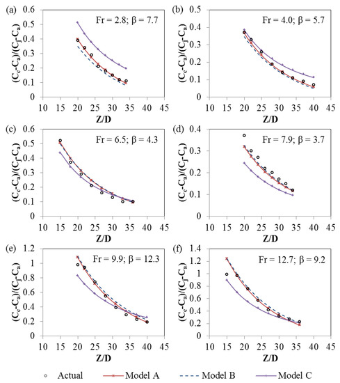
Figure 4.
Actual and predicted concentration profiles: (a) Fr = 2.8; β = 7.7; (b) Fr = 4.0; β = 5.7; (c) Fr = 6.5; β = 4.3; (d) Fr = 7.9; β = 3.7; (e) Fr = 9.9; β = 12.3; and (f) Fr = 12.7; β = 9.2.
For each case, the markers corresponding to the results of Model A are very close to the experimental ones, indicating a good generalization capacity of Model A. The data points of Model B are close to those of Model A. Most of the sub trees in Model B are identical to the counterparts in Model A, implying that these sub trees were the most influential elements, and the remaining sub trees only affected the predictions to a small degree. The Model C points deviate farther from the experimental points, indicating that Model C was over-simplified and thus was not able to predict the jet concentration satisfactorily. It should be noticed with caution that a few MGGP predictions of the dimensionless jet centerline concentration exceeded one, which is not physically reasonable. This reveals the deficiency of data-driven models in strictly ensuring physical rules. The outcome can be improved by training the models with more data with extreme values, such as 0 and 1, or by post-processing the results according to the following bounding criteria:
For the purpose of assessing the original MGGP models, the post-processed predictions are not further discussed herein.
3.3. Quantitative Assessment of Model Performances
For a detailed quantitative evaluation of the performances of the evolved models, the actual and MGGP results at all the data points are plotted in Figure 5. The root-mean-squared error (RMSE) and coefficient of determination (R2) values are also shown in the same plots. The training data points were used to evolve and select the MGGP models, and the testing data points were employed to serve as unseen data points for assessing the predictive capacity of the evolved models. For the training period, the results shown in Figure 5 are consistent with the observations in Figure 3a; namely, Model A (RMSE = 0.037, R2 = 0.968) had the best whereas Model C (RMSE = 0.094, R2 = 0. 798) had the worst performance among the models on the Pareto front in fitting the training data sets for dimensionless jet centerline concentration.
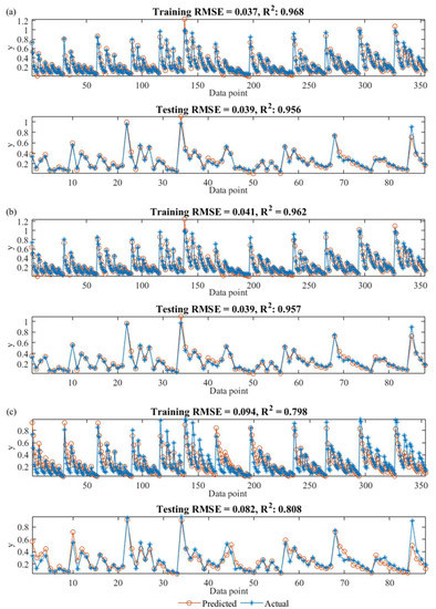
Figure 5.
Comparison of actual and MGGP results: (a) Model A; (b) Model B; and (c) Model C.
For the testing data points, the performances of Model A (RMSE = 0.039, R2 = 0.956) and Model B (RMSE = 0.039, R2 = 0.957) were almost identical. Because of the lower complexity, Model B could be more favorable than Model A if model simplicity is of great importance. The fitting indices of Models A and B for the testing data sets were only slightly different from those for the training data sets, demonstrating that the risks of over-fitting were well controlled. Model C is much simpler than Models A and B, as it only has two genes, but its performance in predicting the dimensionless jet centerline concentration was much poorer at the same time (RMSE = 0.082, R2 = 0.808). This confirms that Model C was under-trained and thus showed consistently poor performance in both the training and testing periods.
To evaluate further the evolved MGGP models, scatter plots of the actual and MGGP predicted results are presented in Figure 6.
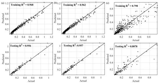
Figure 6.
Scatter plot of the actual and MGGP predicted results: (a) Model A; (b) Model B; and (c) Model C.
Figure 6a shows an excellent match between the measurements and Model A predictions. Only a few symbols appear farther from the identity line. These symbols correspond to the extreme values, i.e., when the output variable is close to 0 or 1, which has been discussed earlier. The symbols for Model B are located near those for Model A with several points deviating slightly farther from the line of agreement than Model A for the training data points. The plots and the R2 values indicated that both Models A and B had less than 5% error in predicting the data sets. Figure 6c shows that the symbols for Model C are distributed in a wider range and the model had about 20% error in the predictions, revealing the poor performance of Model C.
In summary, the detailed comparisons presented above demonstrated that both Model A and Model B can provide very accurate predictions for dimensionless centerline concentrations of vertical buoyant jets subjected to lateral confinement whereas Model C performed poorly. If model complexity is of major concern, Model B is suggested. However, because the evolved models can be easily executed within the environment of MATLAB and Model A has a better generalization capacity for the entire data sets, Model A is focused on hereafter in this paper.
3.4. Comparison with the SGGP Model
The Pareto front plot for the SGGP modeling is presented in Figure 7a. These models were also created through the evolutionary process described earlier in this paper. The only difference between the SGGP and MGGP algorithms was that only one gene was utilized in an SGGP chromosome. It clearly shows that the fitness of each population in SGGP modeling was poorer than that in MGGP modeling. There are only three solutions that fall on the Pareto front and the best one (in a red circle) is selected for further analysis. The mathematical expression for this model is:
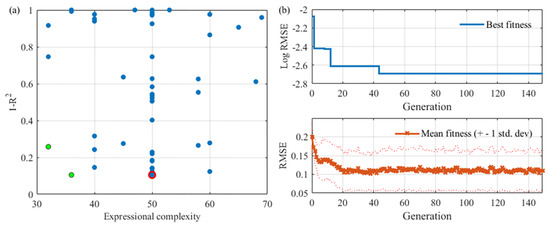
Figure 7.
The Pareto front plot of the evolved SGGP-based models and convergence of the solutions: (a) Pareto front plot; and (b) convergence of the solutions.
Compared with the MGGP models, this SGGP model is much simpler because it only has one gene.
Figure 7b reports the convergence characteristics of the SGGP solutions. Compared with the MGGP modeling, the errors in the SGGP algorithm decreased at a slower rate. The error curve became smoother after about 40 generations, so more SGGP generations were not necessary because they would not noticeably improve the outcome. The mean fitness of the SGGP modeling in Figure 7b is lower than that of the MGGP modeling, indicating that the overall performance of the SGGP algorithm was poorer than that of MGGP.
Figure 8 compares the measured and modeled dimensionless jet centerline concentration at each data point.
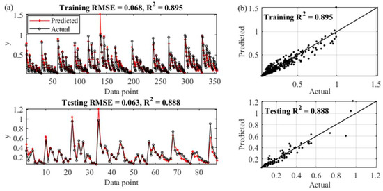
Figure 8.
The actual and SGGP results: (a) results at all the data points; and (b) scatter plots of the actual and predicted results.
The RMSE and R2 values are also reported. For the training data sets, the predictions of the best SGGP model (RMSE = 0.068, R2 = 0.895) were obviously less accurate than the MGGP Models A and B but more accurate than the MGGP Model C. In terms of the testing data sets, the RMSE and R2 values in the SGGP predictions were 0.063 and 0.888, respectively, which also demonstrated that the performance of the SGGP model was better than the MGGP Model C but worse than the MGGP Models A and B.
In summary, the above findings revealed the superior performance of MGGP in evolving an accurate model over the SGGP algorithm. However, the lower RMSE and higher R2 values compared with the MGGP Model C indicate that an SGGP-based model could have higher prediction capability than an MGGP model that is over simplified.
3.5. Comparison with the Existing Empirical Equation
Lee and Lee [10] proposed a regression-based empirical equation for the dimensionless jet centerline concentration, which can be expressed as:
This equation has been used by Lee and Lee [10] and Yan and Mohammadian [19] to estimate and plot the concentration profiles of a laterally confined jet, and the good agreement with experimental results demonstrated the generalization capability of this equation. A scatter plot of the dimensionless jet centerline concentration at each data point calculated using the empirical equation is shown in Figure 9. The MGGP and SGGP data points are also depicted in the same figure. Very surprisingly, the RMSE and R2 values of the empirical results (RMSE = 0.068, R2 = 0.895) were almost identical to those of the SGGP (RMSE = 0.067, R2 = 0.894) results for the entire data sets. A closer examination of the evolved SGGP model and the empirical formulation shows that the two models have a very similar model structure. These observations demonstrated that the SGGP algorithm can easily evolve an explicit model that is as accurate as a regression-based empirical model which normally requires extensive analyses and efforts. The mean absolute errors (MAEs) were also calculated, and the values corresponding to the MGGP, the SGGP, and the empirical models were 0.027, 0.044, and 0.046, respectively. The lower MAE and RMSE and higher R2 values of the MGGP predictions also demonstrated the generalization capacity of the MGGP model.
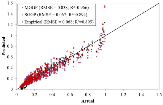
Figure 9.
Comparison of the evolutionary and empirical predictions.
3.6. Prediction Confidence Analysis
Figure 10 presents the prediction confidence analysis result for the best MGGP model (Model A). The analysis was performed using MATLAB’s nonlinear regression prediction confidence interval function, “nlpredci”. This function is based on the symmetric confidence interval approach and can calculate the 95% confidence interval half-width at each data point [34]. The data points shown in Figure 10 have been sorted based on the MGGP prediction from largest to smallest for display purposes. This figure clearly shows that the MGGP predictions followed the overall data trend very well, with the prediction points being uniformly distributed above or below the curve for the experimental data. The confidence range was relatively narrow, with the mean 95% confidence interval half-width being 0.093.
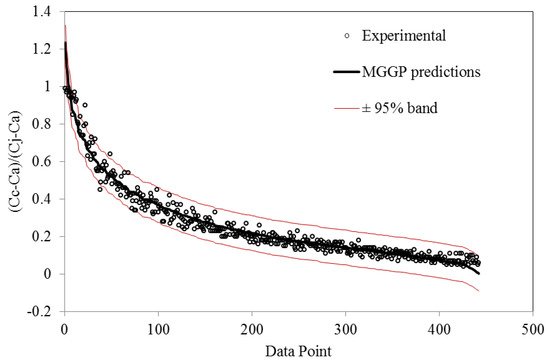
Figure 10.
Prediction confidence analysis of the best MGGP model.
4. Conclusions
In this work, an alternative approach based on MGGP to predicting the initial dilution of vertical buoyant jet subjected to lateral confinement was proposed. Pareto-optimal MGGP-based models were developed to estimate the dimensionless jet centerline concentration using the dimensionless parameters Fr and β. The best MGGP model (Model A) performed consistently well in modeling both the experimental training (RMSE = 0.037, R2 = 0.968) and testing data sets (RMSE = 0.039, R2 = 0.956). Another candidate and less complex MGGP model (Model B) was also found to be accurate in predicting the experimental data (training: RMSE = 0.041, R2 = 0.962; testing: RMSE = 0.039, R2 = 0.957) and may be preferable when model simplicity is of major importance. The best MGGP model had lower errors and higher correlations in fitting the entire data sets (MAE = 0.027, RMSE = 0.038, R2 = 0.966) than the best SGGP model (MAE = 0.044, RMSE = 0.067, R2 = 0.894) and the existing empirical model (MAE = 0.046, RMSE = 0.068, R2 = 0.895). The results of nonlinear regression prediction confidence interval analysis revealed that the mean 95% confidence interval half-width of Model A was 0.093. These results and observations are encouraging. Therefore, the MGGP technique will be applied to other effluent mixing problems in further work.
Author Contributions
Both authors were involved in the data collection, analysis, and interpretation. X.Y. prepared the original draft, and A.M. reviewed and edited the manuscript.
Funding
This work was funded by the Natural Sciences and Engineering Research Council of Canada (NSERC Discovery Grants).
Acknowledgments
The first author, Xiaohui Yan, is a recipient of a scholarship from the China Scholarship Council (CSC).
Conflicts of Interest
The authors declare no conflict of interest.
References
- Gildeh, H.K.; Mohammadian, A.; Nistor, I.; Qiblawey, H. Numerical modeling of turbulent buoyant wall jets in stationary ambient water. J. Hydraul. Eng. 2014, 140, 04014012. [Google Scholar] [CrossRef]
- Jiang, M.; Law, A.W.K.; Zhang, S. Mixing behavior of 45° inclined dense jets in currents. J. Hydro-Environ. Res. 2018, 18, 37–48. [Google Scholar] [CrossRef]
- Jiang, M.; Law, A.W.K. Mixing of swirling inclined dense jets—A numerical study. J. Hydro-Environ. Res. 2018, 21, 118–130. [Google Scholar] [CrossRef]
- Jiang, M.; Law, A.W.K.; Lai, A.C. Turbulence characteristics of 45 inclined dense jets. Environ. Fluid Mech. 2019, 19, 27–54. [Google Scholar] [CrossRef]
- Qiao, Q.S.; Choi, K.W.; Chan, S.N.; Lee, J.H. Internal hydraulics of a chlorine jet diffuser. J. Hydraul. Eng. 2017, 143, 06017022. [Google Scholar] [CrossRef]
- Xu, Z.; Chen, Y.; Pan, Y. Initial dilution equations for wastewater discharge: Example of non-buoyant jet in wave-following-current environment. Ocean Eng. 2018, 164, 139–147. [Google Scholar] [CrossRef]
- Morton, B.R.; Taylor, G.I.; Turner, J.S. Turbulent gravitational convection from maintained and instantaneous sources. Proc. R. Soc. Lond. Ser. A. Math. Phys. Sci. 1956, 234, 1–23. [Google Scholar]
- Manins, P.C. Turbulent buoyant convection from a source in a confined region. J. Fluid Mech. 1979, 91, 765–781. [Google Scholar] [CrossRef]
- Turner, J.S. Turbulent entrainment: The development of the entrainment assumption, and its application to geophysical flows. J. Fluid Mech. 1986, 173, 431–471. [Google Scholar] [CrossRef]
- Lee, A.W.T.; Lee, J.H.W. Effect of lateral confinement on initial dilution of vertical round buoyant jet. J. Hydraul. Eng. 1998, 124, 263–279. [Google Scholar] [CrossRef]
- Shao, D.; Law, A.W.K. Boundary impingement and attachment of horizontal offset dense jets. J. Hydro-Environ. Res. 2011, 5, 15–24. [Google Scholar] [CrossRef]
- Zhang, S.; Law, A.W.K.; Jiang, M. Large eddy simulations of 45° and 60° inclined dense jets with bottom impact. J. Hydro-Environ. Res. 2017, 15, 54–66. [Google Scholar] [CrossRef]
- Gosman, A.D.; Simitovic, R. An experimental study of confined jet mixing. Chem. Eng. Sci. 1986, 41, 1853–1871. [Google Scholar] [CrossRef]
- Khoo, B.C.; Chew, T.C.; Heng, P.S.; Kong, H.K. Turbulence characterisation of a confined jet using PIV. Exp. Fluids 1992, 13, 350–356. [Google Scholar] [CrossRef]
- Shinneeb, A.M.; Balachandar, R.; Bugg, J.D. Confinement effects in shallow-water jets. J. Hydraul. Eng. 2010, 137, 300–314. [Google Scholar] [CrossRef]
- Thong, C.X.; Kalt, P.A.; Dally, B.B.; Birzer, C.H. Flow dynamics of multi-lateral jets injection into a round pipe flow. Exp. Fluids 2015, 56, 15. [Google Scholar] [CrossRef]
- Jirka, G.H. Buoyant surface discharges into water bodies. II: Jet integral model. J. Hydraul. Eng. 2007, 133, 1021–1036. [Google Scholar] [CrossRef]
- El-Amin, M.F.; Sun, S.; Heidemann, W.; Müller-Steinhagen, H. Analysis of a turbulent buoyant confined jet modeled using realizable k–ɛ model. Heat Mass Transf. 2010, 46, 943–960. [Google Scholar] [CrossRef]
- Yan, X.; Mohammadian, A. Numerical Modeling of Vertical Buoyant Jets Subjected to Lateral Confinement. J. Hydraul. Eng. 2017, 143, 04017016. [Google Scholar] [CrossRef]
- Kisi, O. Suspended sediment estimation using neuro-fuzzy and neural network approaches. Hydrol. Sci. J. 2005, 50. [Google Scholar] [CrossRef]
- Hipni, A.; El-shafie, A.; Najah, A.; Karim, O.A.; Hussain, A.; Mukhlisin, M. Daily forecasting of dam water levels: Comparing a support vector machine (SVM) model with adaptive neuro fuzzy inference system (ANFIS). Water Resour. Manag. 2013, 27, 3803–3823. [Google Scholar] [CrossRef]
- Rezaei, F.; Safavi, H.R.; Mirchi, A.; Madani, K. f-MOPSO: An alternative multi-objective PSO algorithm for conjunctive water use management. J. Hydro-Environ. Res. 2017, 14, 1–18. [Google Scholar] [CrossRef]
- Rezaei, F.; Safavi, H.R.; Zekri, M. A hybrid fuzzy-based multi-objective PSO algorithm for conjunctive water use and optimal multi-crop pattern planning. Water Resour. Manag. 2017, 31, 1139–1155. [Google Scholar] [CrossRef]
- Bashiri, H.; Sharifi, E.; Singh, V.P. Prediction of local scour depth downstream of sluice gates using harmony search algorithm and artificial neural networks. J. Irrig. Drain. Eng. 2018, 144, 06018002. [Google Scholar] [CrossRef]
- Moroni, D.; Pieri, G.; Tampucci, M. Environmental Decision Support Systems for Monitoring Small Scale Oil Spills: Existing Solutions, Best Practices and Current Challenges. J. Mar. Sci. Eng. 2019, 7, 19. [Google Scholar] [CrossRef]
- Searson, D.P. GPTIPS 2: An open-source software platform for symbolic data mining. In Handbook of Genetic Programming Applications; Springer: Cham, Switzerland, 2015; pp. 551–573. [Google Scholar]
- Safari, M.J.S.; Mehr, A.D. Multi-gene genetic programming for sediment transport modeling in sewers for conditions of non-deposition with a bed deposit. Int. J. Sediment Res. 2018, 33, 262–270. [Google Scholar] [CrossRef]
- Garg, A.; Garg, A.; Tai, K.; Barontini, S.; Stokes, A. A computational intelligence-based genetic programming approach for the simulation of soil water retention curves. Transp. Porous Media 2014, 103, 497–513. [Google Scholar] [CrossRef]
- Kaydani, H.; Mohebbi, A.; Eftekhari, M. Permeability estimation in heterogeneous oil reservoirs by multi-gene genetic programming algorithm. J. Pet. Sci. Eng. 2014, 123, 201–206. [Google Scholar] [CrossRef]
- Roberts, P.J.; Ferrier, A.; Daviero, G. Mixing in inclined dense jets. J. Hydraul. Eng. 1997, 123, 693–699. [Google Scholar] [CrossRef]
- Lai, C.C.; Lee, J.H. Mixing of inclined dense jets in stationary ambient. J. Hydro-Environ. Res. 2012, 6, 9–28. [Google Scholar] [CrossRef]
- Shao, D.; Huang, D.; Jiang, B.; Law, A.W.K. Flow patterns and mixing characteristics of horizontal buoyant jets at low and moderate Reynolds numbers. Int. J. Heat Mass Transf. 2017, 105, 831–846. [Google Scholar] [CrossRef]
- Pandey, D.S.; Pan, I.; Das, S.; Leahy, J.J.; Kwapinski, W. Multi-gene genetic programming based predictive models for municipal solid waste gasification in a fluidized bed gasifier. Bioresour. Technol. 2015, 179, 524–533. [Google Scholar] [CrossRef] [PubMed]
- Dolan, K.D.; Yang, L.; Trampel, C.P. Nonlinear regression technique to estimate kinetic parameters and confidence intervals in unsteady-state conduction-heated foods. J. Food Eng. 2007, 80, 581–593. [Google Scholar] [CrossRef]
© 2019 by the authors. Licensee MDPI, Basel, Switzerland. This article is an open access article distributed under the terms and conditions of the Creative Commons Attribution (CC BY) license (http://creativecommons.org/licenses/by/4.0/).