1. Introduction
In recent decades there has been a significant increase in the use of nuclear energy. Many nuclear power plants (NPPs) are built on the shores of the seas or oceans in order to provide free access to the water needed for their cooling systems [
1]. Currently, two NPPs are located on the shores of the Gulf of Bothnia in the Baltic Sea: the Swedish station Forsmark and the Finnish station Olkiluoto. Both are located in the southern part of the Gulf of Bothnia (called Bothnian Sea) while it is planned to build another one in the northern part of the Gulf of Bothnia (called Bothnian Bay)—the Finnish NPP ‘Hanhikivi-1’ located on the cape of the same name.
In 2013 a contract was signed between the international division of ‘Rosatom’ Russian State Corporation called ‘Rusatom Overseas’ and the Finnish company Fennovoima for the construction of a 1200-MW NPP ‘Hanhikivi-1’. The official start of the construction was 22 January 2016, but due to a number of problems concerning obtaining the necessary licenses the project’s documentation is still being prepared. It is expected that this stage will be successfully completed and the direct commissioning of the NPP is planned in 2028.
Bothnian Bay is situated between the temperate-marine and continental subarctic climatic zones in the northern part of the Baltic Sea [
2]. The flow of arctic air masses causes harsh winter conditions and in normal years the bay has ice cover. Ice cover presence in Bothnian Bay usually begins in November–December and ends in May–June. Bothnian Bay is characterized by low salinity, the average being 2‰–4‰ with minimum in the northern part of the bay.
Extreme sea levels in the Bothnian Bay are caused by seiches, storm winds and long waves generated by moving atmospheric cyclones. Tidal level oscillations in Bothnian Bay are negligible [
2]. A detailed review of the hydrometeorological conditions and physical processes in Bothnian Bay (as a part of the Baltic Sea) is given in [
2,
3].
The Hanhikivi peninsula is located on the eastern coast of Bothnian Bay. The coastal zone adjacent to the Hanhikivi peninsula is rather shallow and open to Bothnian Bay. The most significant local river in the Hanhikivi area is Pohjoishaara located 6 km southwest off the peninsula with average annual discharge being approximately 30 m3/s.
The assessment of sedimentation rates and bottom sediment transport is a common problem which often arises during the design and operation of hydro-technical structures, dredging works’ planning, assessment of environmental risks due to anthropogenic impacts, etc. Such a task also appeared during the design of the NPP ‘Hanhikivi-1’.
To date, a large number of works aimed on the assessment of sedimentation and sediment transport in different areas of the oceans using various approaches and techniques have been carried out and published. For example, in the work [
4] the estimate of sedimentation in different sections of the Volga–Caspian sea navigation channel was made by means of numerical modeling, and several protection methods were considered. The obtained results showed good applicability of numerical models in estimating and predicting the intensity of sedimentation process in the Volga–Caspian channel under different external forcing. A coupled circulation—wind wave—lithodynamic model for Lake Michigan was described and used in [
5] where a sigma-based Princeton Ocean Model was coupled with lithodynamic and simple wind waves model. Despite the horizontal resolution being rather coarse (5 km), the model results demonstrated good agreement with the available field observations of suspended sediment concentration (SSC) and reproduced the main features of the erosion/deposition processes in the southern part of the lake, although the latter were not validated due to the lack of observation data for the period considered. In [
6] the assessment of sedimentation intensity in the navigation channel of Sabetta port located on the Yamal peninsula was reported. The research was based on the field observations and special processing methods. A volume of sediments coming into the channel due to glacier-induced erosion was also assessed.
The Baltic Sea is a challenging basin in terms of sediment transport assessment since the sea is relatively shallow and meteorological conditions in the area can be rather harsh [
2,
3] thus producing enough energy needed to erode the sediments from the bottom. The area around the Baltic Sea is highly-populated and the processes in the coastal zone attract growing attention. For instance, erosion of the western coast of the Kotlin Island located in the eastern part of the Gulf of Finland was assessed in [
7] using numerical models and field observations and several mitigation measures aimed to protect the beach have been proposed. The period considered was short (only 3 days) and was chosen in order to assess the intensity of coastal erosion during the strongest flood event in 2011, thus a long-term assessment of deposition/erosion intensity was not carried out. Bottom sediment resuspension in the Neva Bay in the easternmost Gulf of Finland was also modeled in [
8,
9,
10] using a coupled modeling system which included a general circulation model, sea ice model, wind waves model and lithodynamic model. Three different sediment fractions were considered and it was shown that the bed-shear stress generated by wind waves was the main factor controlling the resuspension intensity in the Neva Bay, although in some areas the current-related bed-shear stress also had the equivalent impact (regions of Neva river estuary and St. Petersburg dam’s gates). The results were validated by comparison of the calculated and observed SSC and showed good agreement. Sediment transport in the southern Baltic Sea was investigated in [
11] by means of field measurements, and emphasized the strong influence of waves and currents upon the sediment resuspension in shallow waters with a quick response of SSC to the variability of external forcing. In [
12] a modeling study aimed at the simulation of the transport of sedimentary material in the western Baltic was carried out and an analysis of the spatial distribution of the bottom shear stress in response to varying forcing was performed. A significant seasonal variation of the calculated transport rates was reported. An assessment of sediment transport along the eastern coasts of the Gulf of Riga and the Baltic Proper in the Baltic Sea was fulfilled in [
13] using long-term simulations of the nearshore wave climate. Their results showed the presence of several divergence and convergence points along the coast and revealed the main features of the sedimentary system in that region.
Studies aimed to assess sediment resuspension and sediment transport are often primarily focused on its biogeochemical component (e.g., [
14,
15]). A comprehensive modeling study with the aim to investigate the long-term average distributions and transports of resuspended matter and other types of suspended organic matter in the Baltic Sea was performed in [
16] and showed that the model successfully captures the horizontal and vertical distribution of different bottom types in the Baltic Sea.
Summarizing, we can conclude that the use of numerical models properly configured for a specific area gives the correct results in simulation of the sediment resuspension and transport and allows assessment of the rates of sediment accumulation and erosion in different regions. Of great importance is the quality of the current and wind waves fields simulation, as well as adequate representation of the spatial structure of bottom sediments.
A number of recent studies were focused on the risk assessment of external events (e.g., [
17,
18]), the NPP’s severe accident calculation [
19], possible impacts of the NPP to the Bothnian Bay fauna [
20] and on modeling of hydrological conditions [
21] in the area of the Hanhikivi peninsula. In [
22] the frequencies of frazil ice and algae in the Gulf of Bothnian (with conditions similar to that of Hanhikivi) were investigated since these two phenomena can affect the NPP’s seawater intake. However, to date, no studies estimating the sediment resuspension intensity and sedimentation rates occurring in real hydrometeorological conditions in the vicinity of the future Hanhikivi NPP have been reported. In the absence of available field observations of sedimentation rates near the Hanhikivi peninsula the mathematical modeling is the only reliable approach to make at least the preliminary assessment of the above-mentioned processes.
The purpose of this study is to make the preliminary assessment of resuspension intensity and sedimentation rates in the area located in the vicinity of the Hanhikivi cape, where the construction of the NPP ‘Hanhikivi-1’ is planned, under real hydrological and meteorological forcing. The relevance of the work is determined by the obvious need to assess the rates of sedimentation in the area of the construction in order to be able to plan future dredging works, including those in the shipping channel, as well as to help to design the water intake and discharge points which can be affected by sediment accumulation [
23,
24,
25].
2. Materials and Methods
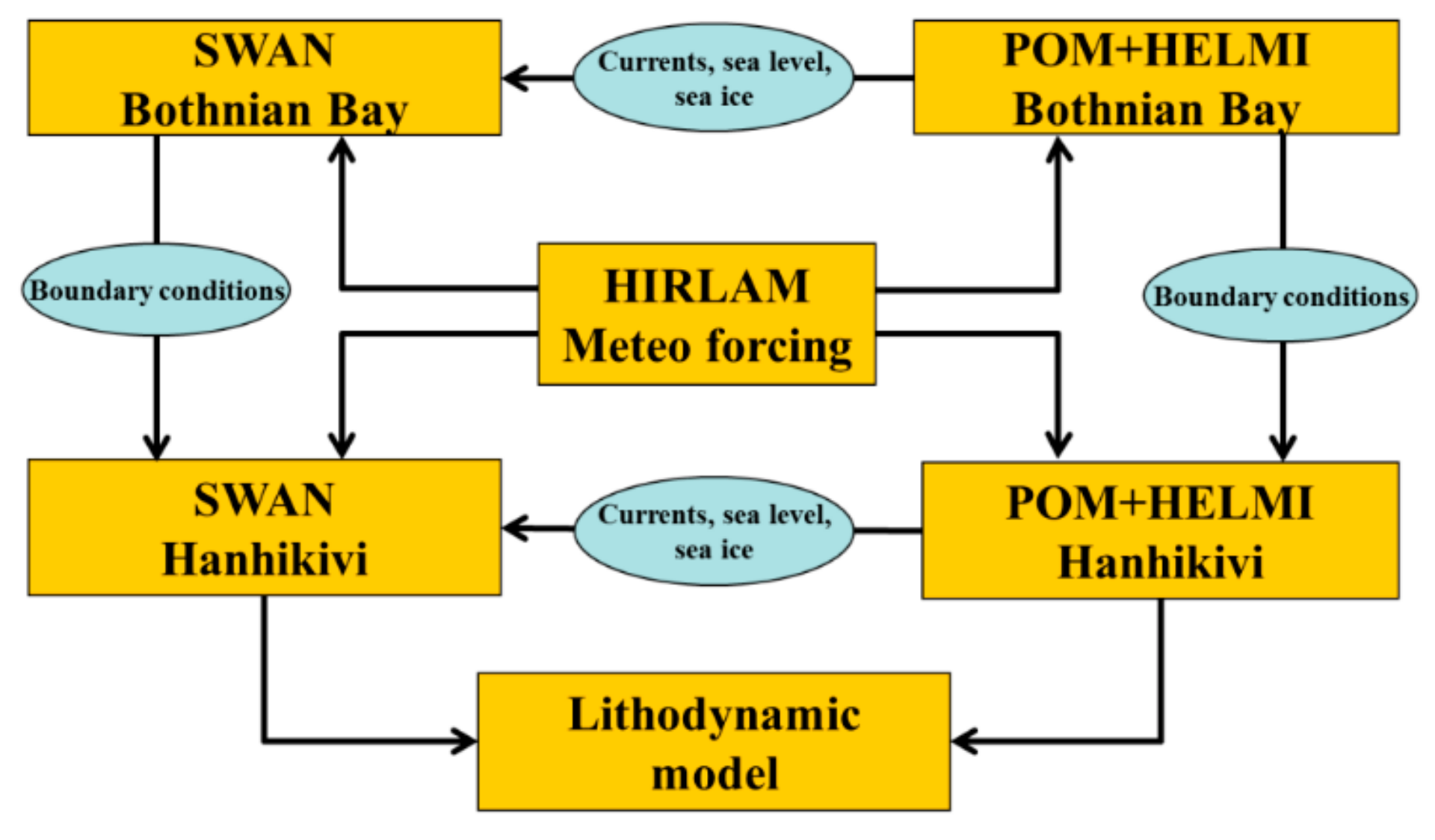
In this work we used a coupled modeling system (
Figure 1) previously developed in [
21] to (assess 1) possible extreme hydrometeorological conditions in the area of the ‘Hanhikivi-1’ NPP construction site (
Figure 2), and (2) the impact of the potential NPP’s thermal effects on the hydrological conditions in the Hanhikivi area. The results obtained showed that the model reproduced the main features of dynamical properties and thermohaline structure and wind waves pattern which was demonstrated in detail in [
21] by comparison with operational model HIROMB (High Resolution Operational Model for the Baltic Sea) and observations at stations located in Bothnian Bay.
2.1. Circulation Model
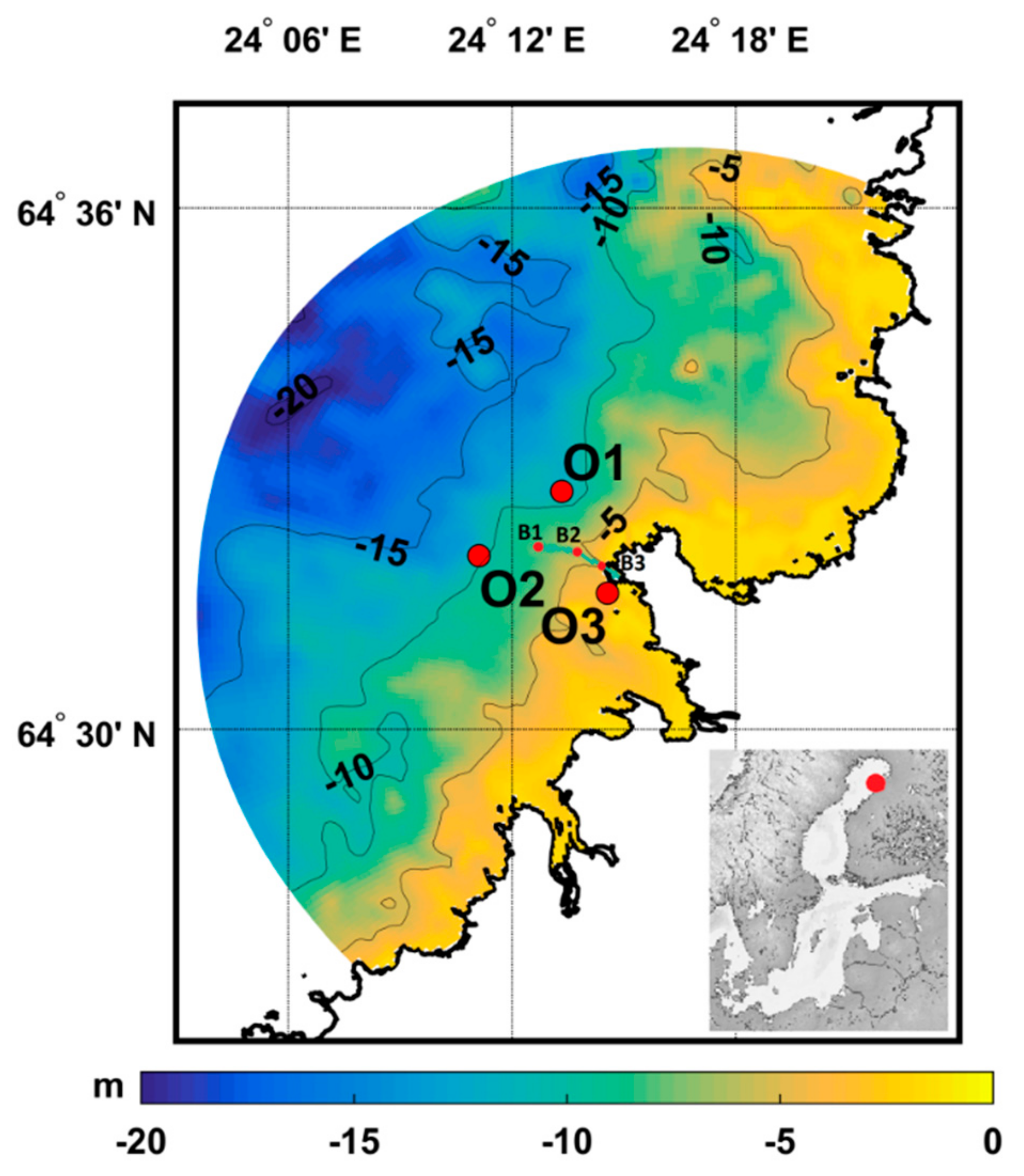
The circulation model used in this study for the Hanhikivi area (
Figure 2) was the Princeton Ocean Model—POM [
26,
27]. In the vertical direction, the model has 12 uniform sigma levels. Such discretization gives a fairly detailed vertical resolution: from about 1.8 m at the open boundary up to 0.5 m at the depth of 5 m and up to 0.15 m in the shallowest areas where the resuspension occurs most intensely. Thus, we believe that the vertical resolution used in the current study is suitable for an adequate simulation of the vertical structure of the flow, water temperature and salinity and also SSC. In the horizontal plane a structured curvilinear quasi-orthogonal computational grid consisting of 142 × 193 nodes is implemented. The horizontal resolution varies within the domain from 35 m to 180 m. The horizontal mesh resolution was chosen in order to resolve the hydro-technical structures near the NPP (port configuration) and the navigation channel, and at the same time to maintain the computational efficiency to run the model for a long period of time.
The use of the sigma-based Princeton Ocean Model for the current study was dictated by the need to make, in addition to the lithodynamics modeling, a complex assessment of the hydrological conditions in the shallow Hanhikivi area, including the extreme maximum and minimum water levels [
21]. For this kind of work, the z-based models are hardly applicable due to the possible problems associated with very low sea level events when the sea level decrease becomes larger than the thickness of the upper grid layer. Such problems force the modeler to enhance the upper layer thickness of the z-based model, thus worsening the vertical resolution. Therefore, the sigma-based model was chosen for the current study in order to be able to simulate a wider range of physical processes and to keep relatively high vertical resolution. As the analysis of the Hanhikivi bathymetry shows, errors associated with a sharp drop in depth may occur only at the borders of the navigation channel (10 m depth). Still, the number of grid cells in the area of the navigation channel (561 grid cells) is small (only 0.3%) compared to the number of wet cells in the entire Hanhikivi model domain (207,504 grid cells) A consistent analysis of the modeled flow patterns in the area of the navigation channel did not reveal any serious discrepancies in the flow field associated with pressure-gradient error.
The model bathymetry was specified according to the Baltic Sea Bathymetry Database (
http://data.bshc.pro) and field measurements in the Hanhikivi area.
The Mellor-Yamada turbulence closure scheme [
28] was used for the vertical turbulent exchange and the Smagorinsky scheme [
29]—for the horizontal turbulent exchange.
At solid lateral boundaries the condition of no heat and salt fluxes was specified and no-slip condition was set for the velocity horizontal components. At the bottom the vertical component of velocity vector, heat and salt fluxes were set to zero. The bottom friction was parameterized as a function of the bottom flow velocity. The initial and boundary conditions are described in
Section 2.5.
Momentum fluxes at the water-air and ice-air interfaces were calculated using the quadratic friction law but with different friction coefficients. Heat and salt fluxes were calculated taking into account the diurnal cycle of short-wave solar radiation [
30]. The outgoing long-wave radiation, turbulent fluxes of apparent and latent heat were parameterized by linear functions of the temperature difference between the air and water surface. In the case of a snow-ice cover presence all heat fluxes were calculated taking into account the concentration and thickness of ice and the thickness of snow on the ice surface.
2.2. Sea Ice Model
The model of viscous-plastic rheology of sea ice HELMI (Helsinki Multi-category Sea-Ice Model) [
31] was used in the present study. Within this model the sea ice is presented as deformed or non-deformed. In the first case, ice is described as consisting of several different categories, in the second case—ridged or rafted ice. The thickness and concentration (compactness) of sea ice of any category are determined by advection, deformation and thermodynamic processes taken into account by the model. The HELMI model allows taking into account the presence of snow on the surface of sea ice. The snow cover in the model is controlled by precipitation, melting, compaction, and the formation of slush.
2.3. Wind Waves Model
To simulate the wind wave field we used the model SWAN (Simulating Waves Nearshore) [
32]—a third-generation spectral wave model specifically developed for wind wave simulation in shelf and shallow coastal areas with complex shoreline configuration. The model can take into account wind forcing, depth-induced wave breaking, refraction, diffraction, ambient currents and sea level oscillations, bottom friction, white capping, wave quadruplets and triads, wave-induced setup, presence of sub-grid obstacles, vegetation and bottom mud layer, and turbulent viscosity. At the solid boundaries the model implements the condition of full wave energy absorption.
SWAN was used in a non-stationary mode with a time step 10 min, with maximal iterations at each time step set equal to 10. The directional resolution was 10 degrees, minimal and maximal frequencies were set equal to 0.04 and 1.0 Hz, respectively. Computational grid was the same as for the circulation model: A structured curvilinear quasi-orthogonal mesh consisting of 142 × 193. The initial and boundary conditions for the wind waves model are described in
Section 2.5.
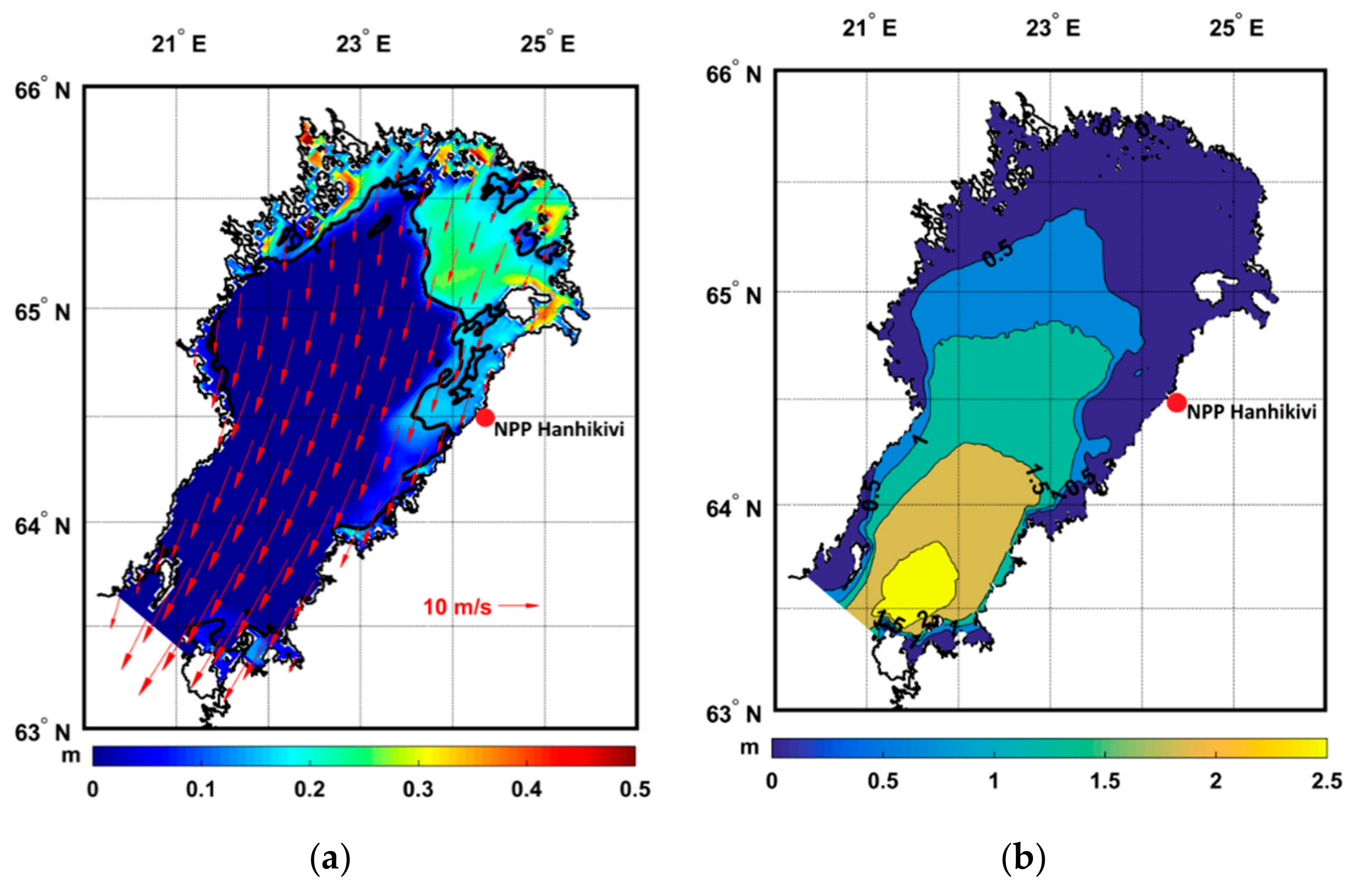
In the present study the model took into account the presence of ice cover—an option which is initially completely absent in the SWAN model. Sea ice hinders or prevents the free generation and propagation of surface waves. Besides the absence of wind waves in the completely ice-covered part of a basin, the presence of ice-cover in other parts of a basin can also limit the wave fetch. An example of a calculated distribution of significant wave height (SWH) in Bothnian Bay partly covered with ice is given in
Figure 3b while
Figure 3a shows the distribution of sea ice thickness, sea ice 0.5-concentration isoline, and also wind pattern at the same moment. The correspondence of the wave field and ice-free region is clear.
A choice of 0.5-isoline of sea ice concentration as the ice edge made it possible to maximally match the results of field measurements of wave height in the vicinity of the Hanhikivi cape [
21]. There is no doubt that such a simple parameterization is a fairly rough approximation of the wave processes occurring in the marginal ice zone, but as a first approximation it allows taking into account the presence of ice cover in the other parts of Bothnian Bay and its influence upon the wind waves field in the Hanhikivi model domain. As follows from
Figure 3, in the area occupied by sea ice there are no wind waves and their generation begins from the position of the ice edge adopted in the model. This effect of sea ice influence upon the wave pattern is important for the nested grids cases such as the one implemented in this study, i.e., even if there is no sea ice in the Hanhikivi model domain (fine grid), the incoming wave height at the open boundary coming from Bothnian Bay is determined by the wave fetch which, in turn, depends on the spatial distribution of the sea ice cover throughout the Bothnian Bay.
2.4. Lithodynamic Model and Field Measurements
To assess the transport of bottom sediments we used a modern lithodynamic model based on verified and well-proven approaches describing the processes of resuspension and transport of bottom sediments [
8]. The model calculates resuspension, variable fall velocity of suspended particles of different fractions, transport of suspended particles in the water column and in the saltation layer, and thickness of the sediment layer. The Exner equation was used for the calculation of the sediment layer thickness change [
33,
34]. The bed-load sediment transport was calculated based on the relationships proposed in [
35,
36,
37]. The resuspension and suspended sediment transport module implements the methods and parameterizations proposed in [
38,
39,
40]. The bed shear stress generated by non-linear interaction of currents and wind waves is calculated by the method proposed in [
41]. Variable in time fall velocity is modeled for each fraction of suspended particles taking into account the current SSC, thus implementing the hindered settling and flocculation effects [
38,
42]. Bottom roughness is determined by the flow regime by using the mobility parameter of the flow (a function of near-bed velocity) and grain size. The diffusivity coefficient for the SSC is taken to be equal to that for salinity. The critical bed-shear stress is constant for each fraction of sediment grains and takes into account the exposure/hiding effects utilized in the multifractional approach [
39]. An unlimited sediment source on the bottom is used in the lithodynamic model in the same way as it was implemented in, e.g., [
5,
34,
40].
The lithodynamic model used in the present study showed good results in simulation the sediment resuspension in the Neva Bay in the Gulf of Finland (Baltic Sea), which was confirmed by the verification of modeled SSC against the measurements made in the bottom and surface layers of the Neva Bay [
8,
9,
10]. The lithodynamic model uses the results of the hydrodynamic model and the wind wave model. The main input data from these models to the lithodynamic model are: depth, sea level rise, current velocity, salinity, ice thickness and ice concentration, turbulent characteristics, significant wave height, wave period, bottom wave orbital velocity and direction of wave propagation.
Unfortunately, the field measurements of SSC were not available for the Hanhikivi peninsula area, as well as any maps of the spatial distribution of the bottom sediments detailed enough to use in the high-resolution model. In fact, the only sediment data available for configuring the lithodynamic model were the measurements of the fractional composition of bottom sediments at three points O1, O2 and O3 (
Figure 2) [
43].
As follows from the measurements [
43], the bottom sediments at three points in the Hanhikivi area consist mainly of sand of different fractions. The density of the sediment particles was set equal to 2650 kg/m
3 in the model as a common value for sand particles used in other modeling studies (e.g., [
44,
45,
46]). As concluded by the analysis of the sampled data, the mineral and granulometric composition of the bottom particles indicates their natural origin and replenishment due to the resuspension and sediment transport by wind waves and currents at relatively shallow depths (0–20 m) around the Hanhikivi peninsula.
According to the recommendations given in [
39], for the relation d90/d10 > 4 a multifraction method should be used since the model considering only one particle diameter cannot adequately describe the resuspension of particles from the graded bed. For the Hanhikivi cape area, as follows from [
43], the distribution of particle sizes leads to the average d90/d10 ratio equal to 7.6, and therefore a multi-fractional lithodynamic model was implemented in the current study.
The lack of data on the spatial distribution of various types of bottom sediments in the Hanhikivi area made it impossible to apply an approach utilizing a predominance of any fraction of particles at a particular region as was done by the authors earlier and showed adequate results in SSC modeling and good agreement with available observations [
8]. The importance of considering the differences in the spatial distribution of the bottom sediments while modeling sediment resuspension and transport in coastal areas cannot be overestimated (e.g., [
47,
48]). This is due to the fact that the physical properties of particles determine such important parameters for any lithodynamic model as the critical bed shear stress at which particles begin to move, bed roughness, bed shear stress, fall velocity, bed reference concentration, etc. In the current study the fractional composition of sediments had been measured only at three points closely located to each other, that is why it was impossible to determine the spatial distribution of bottom sediments throughout the entire Hanhikivi model domain.
To date, a number of studies have used or provided some information about the types of bottom sediments in the Baltic Sea [
12,
16,
49,
50,
51], although none of them provided information detailed enough to distinguish the spatial differences of sediment distribution in the small Hanhikivi domain. As a result, we decided to modify the existing lithodynamic model by making it fully multi-fractional in order to use the available but very limited observational data, thereby introducing the regional Hanhikivi-related features into the model. We are talking about not only taking into account several different fractions of bottom particles as was done earlier (the areas of different bottom sediments had a homogeneous composition in [
8,
9,
10]), but also about taking into account several fractions of particles at each model grid point. In other words, the model has become fully applicable for working with an arbitrary mixture of particles of different sizes. However, due to the lack of complete data on the spatial distribution of bottom sediments over the model region a uniform field of bottom sediment mixture was set, consisting of seven different fractions. This number of fractions was chosen on the basis of the real fractional distribution of particles provided by field measurements in the area of the Hanhikivi peninsula and the recommendations given in [
39]. Of course, the use of such spatially homogeneous field is a rough assumption since in real conditions the fractional composition of bottom sediments in the direction from the coast to deeper waters varies considerably [
8,
16]. Therefore, the model results in the present study are expected to somewhat overestimate the SSC and the change of sediment layer thickness in the very shallow coastal zone and to underestimate these quantities in deeper areas. Still, the use of the spatially homogeneous distribution of sediment mixture consisting of several different sediment fractions showed its good applicability in an analogous modeling-based assessment of sediment transport in the Volga–Caspian Shipping Channel [
4] characterized by similar conditions (shallow depth, seasonal presence of ice cover, events of harsh meteorological conditions, different fractions of bottom sediments, absence of tides but presence of seiches and storm surges).
2.5. Initial Conditions, Boundary Conditions and Model Parameters
The numerical experiment’s design was as follows: first we performed numerical experiments in order to calculate sea level, currents, water temperature and salinity, sea ice characteristics and wind waves in the entire Bothnian Bay (
Figure 3) on the coarse grid with horizontal resolution of 1 nautical mile for the period 2010–2014. The initial and boundary conditions for Bothnian Bay circulation and sea ice models were taken from the operational model HIROMB [
52], while zero initial and boundary conditions were specified for the Bothnian Bay wind waves model. Such initial and open-boundary conditions for Bothnian Bay wind waves model were used because: (1) the wind waves’ field in Bothnian Bay adjust to external meteorological forcing rather quickly and (2) the impact of the incoming wind waves plays an important role only in the southern part of Bothnian Bay and its contribution to the wind wave pattern in the vicinity of the Hanhikivi peninsula is negligible, as was shown in [
21]. Thus, for the beginning of 2014 all required initial and boundary conditions for the fine-grid nested Hanhikivi model were prepared from the previous four-year run of the coarse-grid Bothnian Bay model. It should be emphasized that the lithodynamic model was not run during Bothnian Bay simulations, thus no initial and boundary conditions were prepared for lithodynamic variables of the fine-grid Hanhikivi model.
After that, we performed a model run for the much smaller internal nested domain (Hanhikivi area, fine grid) for the whole 2014 year taking the initial and boundary conditions from the previous entire Bothnian Bay calculation.
The initial condition of no wind waves in the entire Hanhikivi domain was adopted. At the solid boundaries the model implements the condition of full wave energy absorption. At the open boundaries, in the case of outgoing waves, a radiation condition is specified. The incoming wave spectrum obtained from the previous entire Bothnian Bay simulations was specified along the open boundary.
Zero suspended sediment concentration in the entire Hanhikivi domain was specified as the initial condition for the lithodynamic model, the boundary conditions being zero SSC for the inflow and radiation condition for outflow. By the beginning of the 2014 year the change of sediment layer thickness was zero and later on it was evolving during the simulation as a result of the convergence and divergence of sediment fluxes (including sediment resuspension, settling, turbulent mixing and advection).
Due to the lithodynamic model’s assumption of infinite sediment source at the bottom without vertical sediment structure (as a result of the absence of data on the spatial distribution and vertical structure of bottom sediments in the Hanhikivi area and relative simplicity of the lithodynamic model itself) there is not much sense conducting a spin-up model run since the equilibrium state cannot be achieved in these circumstances. The lithodynamic model used in the current study is rather simple, it does not take into account the vertical structure of the sediment layer and, in fact, cannot reproduce such kinds of processes as bed armoring, which can prevent sediment resuspension in certain areas after some time of external forcing.
For all model runs the external meteorological forcing which included the temporally and spatially varying fields of wind, atmospheric pressure, air temperature and humidity, cloudiness and precipitation rate, was taken from the operational atmospheric model HIRLAM (High-Resolution Limited Area Model,
http://hirlam.org).
For the Hanhikivi circulation model, a climatic river discharge equal to 30 m
3/s was used for the Pohjoishaara River located within the Hanhikivi model domain [
53]. The salinity of the river water was set equal to zero, the temperature—equal to that in the nearest model cell of the coastal zone due to the lack of data on the actual water temperature in the river. The area around the Hanhikivi peninsula and especially its coastal part where the Pohjoishaara River flows into the bay (see
Figure 2) is very shallow, and therefore we assume that the water temperature in that small area adjusts quickly after having been discharged from the river.
No sediment load was considered from the Pohjoishaara River due to the lack of available data of turbidity or SSC. Some data about rivers flowing into Bothnian Bay can be found in [
54,
55,
56], but information related to the Pohjoishaara River is absent. The runoff of the Pohjoishaara River is rather small (30 m
3/s) compared to, for example, Neva River runoff (app. 2500 m
3/s) where the riverine flux of suspended sediments should be taken into account when simulating the suspended sediment transport in the shallow Neva Bay [
8]. We assume that the influence of the small runoff of the Pohjoishaara River does not significantly affect the thermal structure of the Hanhikivi area waters [
21], as well as the distribution of SSC in the vicinity of the peninsula. Unfortunately, to prove or contradict this assumption the reliable field measurements in the estuary are required which are not currently available.
Despite the fact that the models used in the present study involve dozens of parameters and coefficients which can hardly be fully listed here, we have summarized the main ones in
Table 1 where the basic coupled Hanhikivi model parameters are presented, including time steps and grid discretization. We also highlight critical bed shear stress and fall velocity for each of 7 fractions considered in the lithodynamic model since these characteristics have a great importance in the model. We would like to emphasize, that the fall velocities presented in the
Table 1 are the initial values that can be slightly modified during the calculations due to the hindered settling and flocculation effects [
38,
42]. The critical bed shear stress values do not simply increase with increasing grain diameter due to hiding and exposure effects [
39].
3. Results and Discussion
A main model run was carried out for the entire 2014 in order to determine the intensity of the bottom sediments resuspension and the main areas of sediment accumulation in real hydrometeorological conditions with permanently changing real external forcing during a relatively long period of time. Considering the fact that the main natural mechanism leading to the sediment resuspension in coastal areas is the wind waves, it is obvious to expect that intense sediment resuspension will be observed in those years when the ice cover period is minimal. The choice of 2014 was made because it was the warmest year during the period 1993–2014 for which meteorological field measurement data for the Hanhikivi peninsula area (station Raahe) were available [
43,
53]. For comparison, in 2014 the sea ice cover in the area near the Hanhikivi peninsula was observed from the beginning of January till the beginning of April, whereas in 2010 (severe winter) the ice cover was present from the beginning of December until the beginning of May.
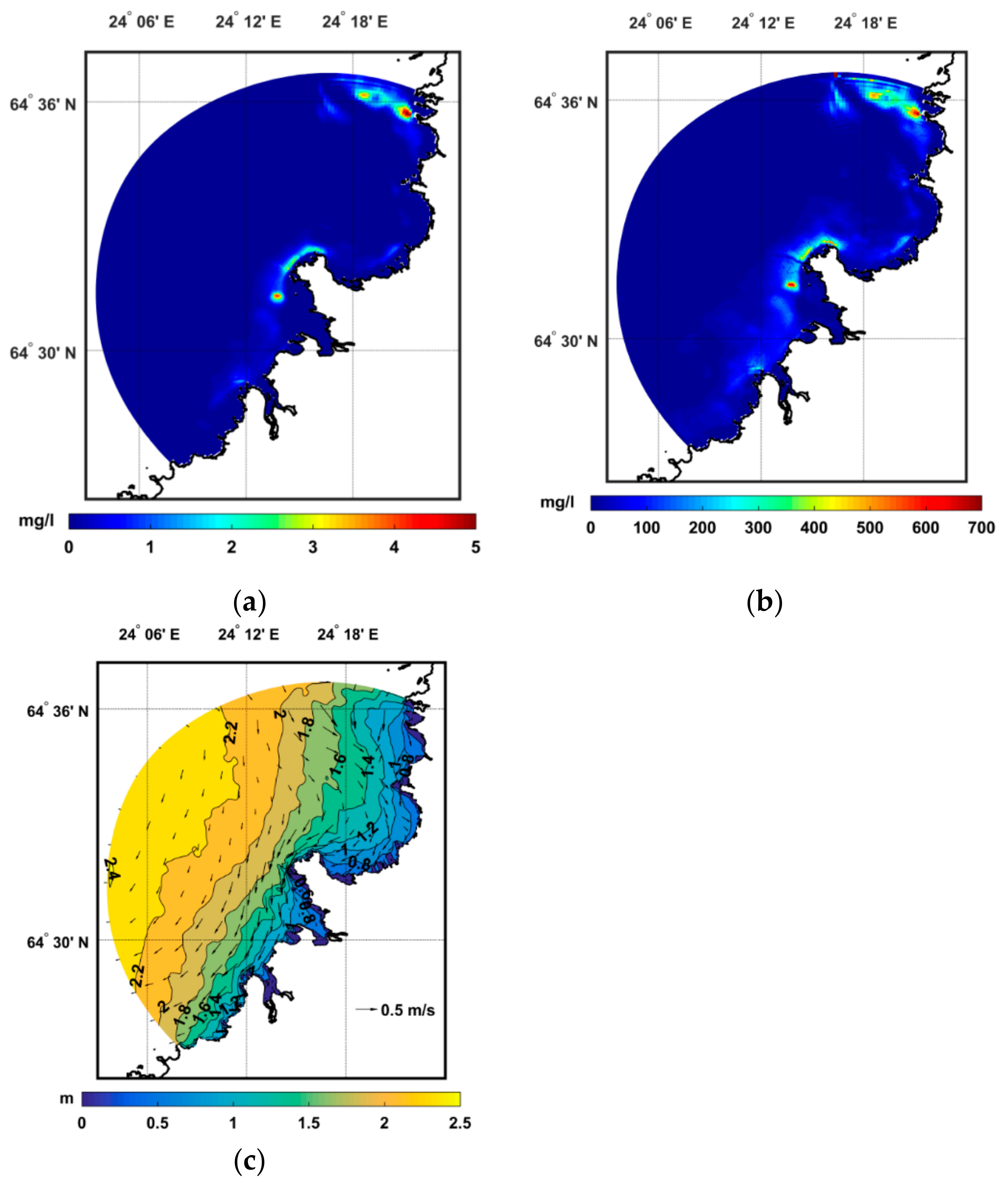
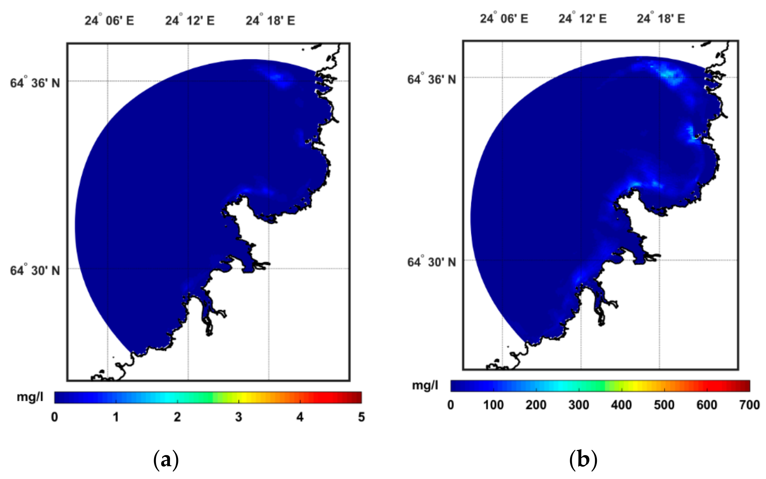
Figure 4 and
Figure 5 present the model results of the SSC in the bottom and surface layers for different dates in 2014. Two situations are shown (16 June and 27 September) with rather high concentrations of suspended matter due to high wind waves and a strong coastal current. Note that the scale ranges are very different for surface and bottom layers. A SWH pattern and surface current velocity distribution are also shown.
The presented results show that the difference between the bottom and surface SSCs is about two orders of magnitude for the zones where resuspension occurs most intensely: the area located in the vicinity of the Hanhikivi cape and the shallow region in the northeast part of the model domain. Such differences between bottom and surface SSCs are common for the observed sediment composition—the main types of bottom sediments in the Hanhikivi area are sands with a rather high gravitational fall velocity (see
Table 1) compared to, for example, silt or clay bottom sediments which form more uniform vertical distribution in the water column when eroded from the bottom [
8]. The obtained values of the suspended sediments surface concentration are in the same order of magnitude (2–7 mg/L for sand particles) as surface SSC in the Neva Bay during strong winds and relatively high SWH [
8,
10]. Somewhat higher values of surface SSC were reported in [
5] for the southern part of Lake Michigan (5–25 mg/L) and in [
57] for the North Sea (10–30 mg/L). But in these studies smaller sediment grain sizes were considered in the corresponding models: uniform sediment grain size of 30 μm for Lake Michigan and three fractions (with diameters smaller than 63 μm) for the North Sea. It is obvious that the sediment grain size is of crucial importance for any lithodynamic model since it determines such characteristics as critical bed shear stress and settling velocity. Thus such comparison is made here not to show the similarities in conditions and SSC in all above-mentioned locations but to demonstrate that the SSC results obtained in the present study for the Hanhikivi area are of realistic values. The need to somehow compare our results with those observed in similar conditions is dictated by the necessity to somehow validate the model in the absence of field observations of SSC in the Hanhikivi area.
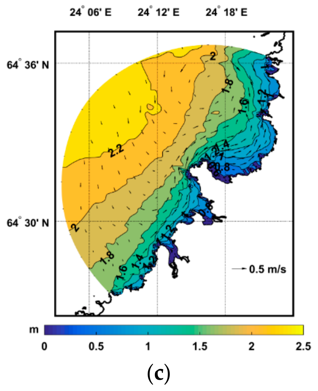
It is always advisable to carry out the analysis of the resuspended matter distribution considering the distribution of the main physical factors affecting this process. In this case those are wind waves and current velocity.
Figure 4c and
Figure 5c show the spatial distributions of the SWH on 16 June and 27 September, respectively. In terms of wind waves, they are generally similar for both cases presented: SWH reached 2.0–2.5 m in the seaward part of the region and about 1.5 m near at the Hanhikivi cape. Wind waves often play the major role in the sediment resuspension process in shallow coastal areas, and so at first glance it is somewhat strange to see quite significant differences in SSCs for both dates. The surface SSC near the Hanhikivi cape reached 2–3 mg/L on 16 June while the surface SSC was only 0.8–1.0 mg/L in the same region on the 27th of September. We note that the wave heights in both cases were approximately the same in this area, and on the 27th of September SWH was even slightly higher. The reason for the differences in the resuspension intensity is that the coastal area near the Hanhikivi cape is characterized by the presence of strong longshore currents generated during strong winds. The selected dates show the cases with strong currents of the opposite direction. The maximum surface velocities reached 50–60 and 40–50 cm/s on 16 June and 27 September, respectively.
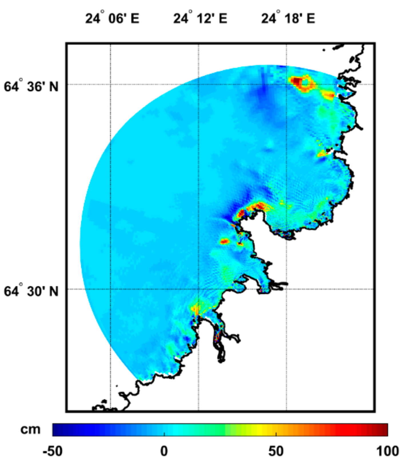
Figure 6 shows the change of sediment layer thickness occurred after the annual period of realistic external forcing (2014).
As seen from
Figure 6, the main areas of sediment accumulation were located the coastal band at the Hanhikivi cape and the shallow region to the northeast off the peninsula. In addition, almost entire shoreline was also a subject to sediment accumulation but in a much lesser degree. It is also worth mentioning the areas where the erosion process occurred—the area to the north from the Hanhikivi cape’s accumulation zone, from which, apparently, the bottom sediments moved closer to the coast under the action of waves and currents.
Beside the spatial distribution of sediment accumulation and erosion zones throughout the area, the sediment processes occurring in the navigation channel are also of interest. The ship channel is 10 m deep and connects the Hanhikivi peninsula with more distinct seaward waters.
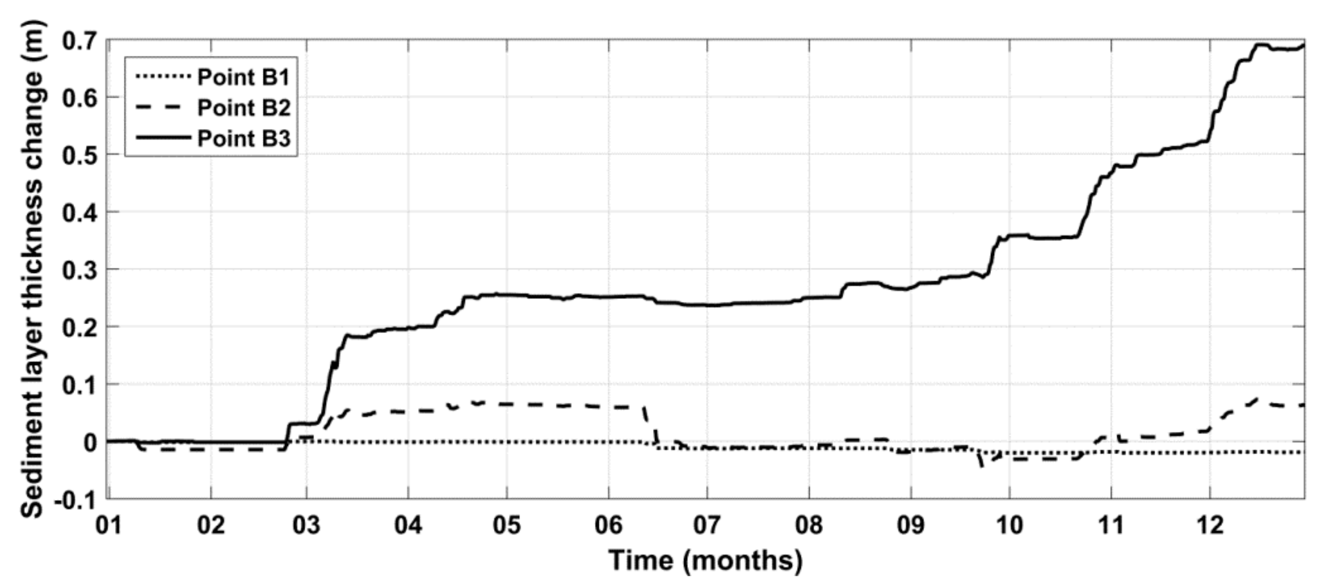
Figure 7 shows the annual change of the sediment layer thickness at three points B1, B2, and B3 located in the offshore, middle, and coastal parts of the channel, respectively (see
Figure 2).
As seen from
Figure 7, sediment accumulation in the offshore part of the channel (point B1) was absent, and even slight bottom erosion equal to 2 cm/year occurred. In the middle part of the channel (point B2) the sedimentation intensity was about 10 cm/year, but it was strongly varying during the year—there were both periods of heavy sediment accumulation (late February–mid March, November–December) and periods of intense erosion of the bottom sediment layer (mid of June, end of September). The coastal part of the navigation channel (point B3) was characterized by the highest sediment accumulation rates. At the end of the year, the thickness of the sediment layer in point B3 increased by 70 cm. The intensity of the accumulation process in the coastal part of the channel changed significantly during the year. The maxima occurred in the middle of March, when the water area became free of ice and also at the end of the year. The results obtained in the present study correlate well with similar modeling-based sedimentation assessment made for the Volga-Caspian channel in [
4] where the sedimentation intensity equal to 1.14 m/year was reported after a year of external forcing.
As follows from the analysis of model results, the sediment accumulation intensity peaks in the navigation channel occurred during the periods of highest wind speeds reaching 14–18 m/s.
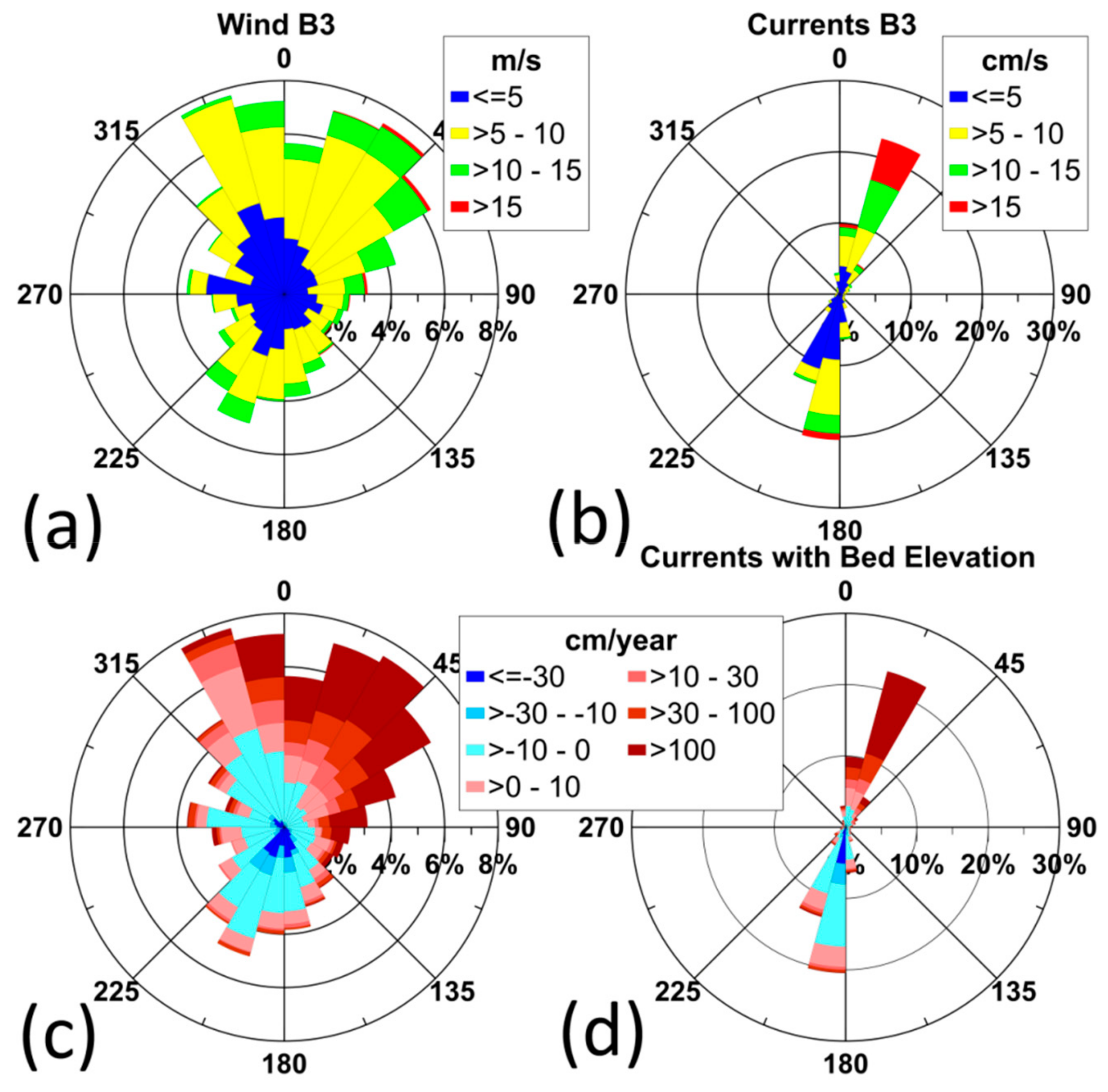
Figure 8 demonstrates the directional distribution of wind and modeled depth-averaged currents at the point B3 located in the coastal part of the navigation channel where the highest rates of sedimentation throughout the channel were obtained. The sedimentation rates together with wind and current roses are also presented.
Figure 8a shows that the winds directed to NE were among the most frequent throughout the 2014 year and reached speeds over 15 m/s. As follows from
Figure 8c, these winds led to significant sedimentation at the point B3 by means of wind waves and currents (
Figure 8b) which resuspended bottom sediments and partly relocated them into the channel. The directional distribution of depth-averaged currents (
Figure 8b) clearly shows the dynamical regime in the vicinity of the Hanhikivi peninsula occurred in 2014. Some features of this regime have already been shown in
Figure 4c and
Figure 5c by means of snapshots of modeled wave and currents fields. As follows from
Figure 8d, the NNE-directed currents mainly led to accumulation of sediments in the navigation channel. The thickness of the sediment layer at the point B3 sometimes decreased during the periods of the south-directed currents. Thus, we would like to emphasize that it was not always only the high wind speed that causes intense resuspension of sediments with their further transport. Equally important was the direction of the wind.
4. Conclusions
A preliminary assessment of the bottom sediments resuspension and sedimentation rates in the eastern part of Bothnian Bay near the Hanhikivi peninsula, where the construction of the ‘Hanhikivi-1’ NPP is planned, has been carried out for the first time by means of numerical modeling for the 2014 year. Temporal and spatial features of the sedimentation process near the Hanhikivi cape have been analyzed.
A brief description of the modeling system used in the current study is presented with a detailed description of the modified multifractional lithodynamic model. Results of field measurements aimed to determine the fractional composition of bottom sediments at three points located in the coastal zone near the Hanhikivi cape are also presented.
The impact of currents upon the sediment resuspension in the vicinity of the Hanhikivi cape has been discussed.
Based on model results, it has been found that the main sediment accumulation areas are located along the coastline of the Hanhikivi cape, and also the shallow region to the north-east off the cape.
Sediment accumulation rates in the navigation ship channel have been estimated. It was found that sediment accumulation in the offshore part of the channel was absent while erosion was about 2 cm/year. In the middle part of the channel the sedimentation rates were about 10 cm/year. The coastal part of the navigation channel was characterized by the highest sedimentation rates—sediment layer thickness had increased by 70 cm by the end of the year.
It should be noted that the values obtained for the change of sediment layer thickness contain a serious assumption made in the lithodynamic model. The spatial homogeneity of the bottom sediment mixture has been adopted in the model. This assumption was made due to the lack the data on the distribution of bottom sediments in the vicinity of the Hanhikivi cape. The use of such sediment field is certainly a rather rough assumption since in real conditions the fractional composition of bottom sediments varies in the direction from coast to deeper areas due to the differences in the hydrodynamic forcing exerted on the bottom by currents and waves. Thus, the model results are likely to overestimate the SSC and the changes of sediment layer thickness in the very shallow coastal zone and to underestimate these quantities in deeper areas.
A serious improvement of the model formulation and corresponding results and estimates will be possible if additional and more comprehensive in situ measurements of the spatial distribution of bottom sediments are carried out over a larger coastal area around the Hanhikivi cape.

 ,
, 


