Abstract
Most physical model tests carried out to quantify wave overtopping are conducted using a wave energy spectrum, which is then used to generate a free surface wave time series at the wave paddle. This method means that an infinite number of time series can be generated, but, due to the expense of running physical models, often only a single time series is considered. The aim of this work is to investigate the variation in the main overtopping measures when multiple wave times series generated from the same spectrum are used. Physical model tests in a flume measuring 15 m (length) by 0.23 m (width) with an operating depth up to 0.22 m were carried out using a stochastic approach on two types of structures (a smooth slope and a vertical wall), and a variety of wave conditions. Results show variation of overtopping discharge, computed by normalising the range of the discharges at a certain wave condition with the maximum value of the discharge in the range up to , when the same wave time series is used, but this range increases to when different time series are used. This variation is found to be of a similar magnitude to both the one found with similar experiments looking at the phenomena in numerical models, and that specified by the confidence bounds in empirical methods.
1. Introduction
The coastal region has significant global economic and societal importance, leading to the extensive construction of coastal structures to defend these areas from the effects of wave action and currents. These structures are subjected to a variety of hydraulic processes, one of the most important and extensively studied being wave overtopping, due to the danger it poses to the people, property and infrastructure being protected. Therefore, the prediction of wave overtopping is crucial and it can be achieved using three established methods [1]: by using empirical formulae derived from large datasets of laboratory and field measurements (e.g., [2,3,4,5]); by using scaled physical model tests carried out in laboratories (e.g., [6,7,8,9,10,11,12,13]) some of which were included in the CLASH dataset [14] to calibrate formulae and neural network tools; or by simulating the hydraulic response of a structure using numerical models (e.g., [15,16,17,18,19,20,21,22]). Over the years, extensive research has been carried out into all of these methodologies; nonetheless, they are not perfect design tools, and they require further improvement.
Uncertainty in wave overtopping prediction has many sources. For example, even the methodology used by different laboratories introduces a variability in overtopping measures. This aspect was investigated by [14] and a complex method for dealing with it was introduced. Here, we are interested in one particular aspect that has recently gained attention, the quantification of the uncertainty induced by the generation of individual sequences of waves from the same energy density spectrum. This uncertainty occurs due to the fact that from every energy spectrum an infinite number of different waves sequences can be generated, simply by changing the initial seeding of the random phase distribution. Evidence that this plays an important role in the variability of results of numerical models was first given in studies by [23] for the prediction of run-up and [24] for overtopping which used a limited number of tests and waves, but showed that the parameters of overtopping can vary significantly with the seeding used. Subsequent work, using numerical models, by [25,26] carried out an extensive Monte Carlo analysis, and concluded that higher uncertainty was observed in both the overtopping discharge and the individual overtopping volumes when the probability of overtopping was less than , with uncertainty decreasing as overtopping increased. Work by [27] also investigated a similar problem in the study of breakwater failure due to wave–structure interaction.
Uncertainty in the context of physical modelling was investigated in a number of works [6,8] with [6] first analysing this particular source of variability by performing a limited number of tests on a vertical wall, using different wave sequences generated from the same energy density spectrum. The work found that variability, due to the wave seeding, of the overtopping measured ranged from approximately between and , depending on the exact parameter of interest. Further work by [28] examined this same variability by considering a small set of laboratory experiments on a specific type of structure, namely a rubble mound breakwater. Similarly to numerical model results, it was shown that, when the probability of overtopping was less than and for (where is the structure crest freeboard above the still water level and is the spectral significant wave height at the structure toe), the variability was higher, decreasing as overtopping discharges increased. However, both of these studies were limited to a single structure type, which makes it impossible to fully extrapolate the results of the variability to other typical designs.
Although physical modelling is generally considered to be a reliable approach for the prediction of overtopping at coastal structures, when complex layouts or wave conditions are considered, the study by [28] identified that further research is required. A further motivation to the present study is given by the fact that this type of uncertainty in the laboratory tests is implicitly included in empirical formulae, which provide confidence bounds of the overtopping prediction to quantify uncertainty coming from all sources. Currently, it is not known how much of this uncertainty is generated simply by the seeding.
The purpose of this work is to address this gap by carrying out an extensive experimental analysis. A stochastic approach was used to quantify this source of uncertainty in physical models. Accordingly, a large number of overtopping experiments were carried out, by randomly altering the initial seeding values used to generate the wave time series for each experimental run. To increase the scope of this work, two different structure types were considered, one a smooth slope, and one a vertical wall, both representative of many existing coastal defence structures found around the world. In addition, a variety of wave conditions were considered, so that results can be extrapolated to different levels of overtopping.
As noted in [28], the study of uncertainty using multiple tests with different seeding forces to use small (i.e., with depth at generation of the order of a fraction of 1 m) scales. This inevitably introduces scale effects. Note that the experimental set-up in [28] is similar to the present one in terms of hydraulic parameters (e.g., water depth, wave characteristics.
When operating on a small scale, one of the most important effects on wave overtopping is given by the much lower air content in breaking waves interacting with the structure. A way of dealing with scale effects in overtopping prediction is provided by [5] in the form of a correction factor for the predicted overtopping discharge. However, it should be noted that, in the experiments presented in [28], when the variability of the results was analysed, scale effects acted in the same way in all tests; therefore, experiments can be compared among each other. However, the role of scale effects in affecting the variability remains unknown. Smooth structures were chosen so that the effect of the armour in terms of roughness and air entrainment was not present.
The paper is organised as follows; the following section describes the experimental set-up and instrumentation. Section 3 provides details about the test programme and experimental procedure, including information regarding the limiting of laboratory effects. Section 4 describes and analyses the effect that altering the seeding has on a number of overtopping parameters. Section 5 discusses the main points identified in the results; and finally Section 6 presents the overall conclusions of this research.
2. Experimental Set-Up
2.1. Flume Set-Up
The experiments were carried out in the wave flume at the University of Nottingham, which is approximately 15 m in length, 0.23 m in width and has an operating depth of up to 0.22 m. It is fitted with a piston type wave generator with active absorption (developed by HR Wallingford). The bottom of the flume is flat, but, for these experiments, a stainless steel foreshore was placed, starting at 6.75 m from the neutral position of the wave maker at 0 m. This allowed for the generation of depth-limited waves without the onset of wave breaking at the wave paddle. This foreshore was 4 m long in total, with a steeper 1 m section closest to the paddle end, followed by a 3 m section with a gradient of 1:50, which met the toe of the structures tested.
Two different overtoppable structures were independently placed in the flume on separate occasions for testing, namely an impermeable smooth slope with a gradient of 1:2.55 and a vertical wall. Both of the structures tested had an identical freeboard ( m). An overtopping tank was installed in the flume on the leeward side of the structures; water that overtopped the structures was directed into this tank. The full set-up of both experiments is detailed in Figure 1, with photographs of the two different structures shown in Figure 2.
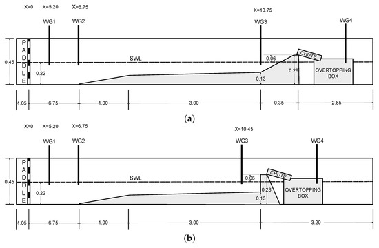
Figure 1.
Indicative layouts of the physical models (not to scale). (a) smooth sloped structure; (b) vertical wall structure.
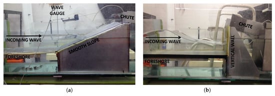
Figure 2.
Photographs of the University of Nottingham experimental set-up. (a) smooth impermeable slope; (b) vertical wall.
2.2. Wave and Overtopping Measurement and Analysis
The water free surface () was measured along the flume using three wave gauges (1–3, see Figure 1 for their positions). was located close to the paddle within the flat bed section, was at the toe of the foreshore where waves were fully developed, and was located close to the structure and was used to obtain the wave conditions at the toe. These wave gauges were of resistance type, and, due to their high sensitivity to laboratory conditions [29], they were calibrated twice daily during these experiments. This was to decrease the likelihood of the calibration affecting the reading, as water temperature changed throughout the day.
A standard procedure for measuring the overtopping volumes was used. A chute was placed just behind the crest of the structure. As water overtopped the structure, it entered this chute, and then flowed down into the overtopping tank situated at a distance behind the structure. The tank was constructed from stainless steel, measuring 0.5 m long by 0.22 m wide by 0.30 m deep, with a false wall in the centre, which allowed water to pass underneath, and dampened oscillations on the water surface in the rear section. Two chutes were used for these experiments, one of width 7.3 cm and one of width 22.0 cm, with the most appropriate one chosen depending on the expected discharge based on the empirical prediction. Using the wider chute for lower discharges allowed for more accurate measurements of the small individual events, whilst using the narrow chute for higher discharges removed the issue of the tank becoming full before the experimental run was complete. A wave gauge () was placed in the rear section of the tank to detect any changes in the water depth due to incoming wave overtopping. With the dimensions of both the chute and the box known for each experiment, these water depth changes were transformed into overtopping measures.
Changes in the water depth within the tank between the start and end of each experimental run were used to calculate the mean overtopping discharge, for each experiment. To calculate the probability of overtopping and the individual overtopping volumes , the time series of the individual overtopping volumes, i.e., the sudden changes in water depth multiplied by the surface area of the tank, was analysed. The original signal was filtered using a low pass digital filter. A peak detection method was then used to detect each individual overtopping event; the volumes were then calculated by working out the difference between subsequent peaks. However, due to the noise within this data, caused by oscillations in the water surface, there was still some residual uncertainty in the volume values calculated. Another limitation of this methodology that was followed was that it is quite possible that small overtopping events were not detected in the signal, hence lost, particularly in the high overtopping conditions, where multiple occurrences of overtopping took place in quick succession. This does not affect the discharge computations.
3. Test Programme
3.1. Incident Wave Conditions
This work is divided into two sets of experiments—one set carried out using the smooth slope structure, whilst the other set was carried out using the vertical wall. The irregular waves generated by the wave paddle in all tests used a JONSWAP spectra with a peak enhancement factor of . For each structure type, four different wave conditions were tested. These were specifically chosen to ensure a range of overtopping magnitudes.
A number of wave conditions were initially tested, with three of those (, and ) being deemed suitable for both of the structural geometries and were therefore tested with both structures in position. Due to the differing wave–structure interaction between the two different types of structure, the fourth wave condition for each case needed to be different. For the smooth slope, a small wave condition resulting in low overtopping () was chosen; however, this resulted in no overtopping of the vertical wall structure, and therefore it could not be used for this structure. Instead, a further wave condition was chosen for the vertical structure only (). This resulted in enough wave overtopping to allow statistical analysis of the variation.
A summary of the incident target wave conditions, used in these tests, prescribed at the paddle are shown in Table 1. Here, is the spectral significant wave height at the paddle, is the mean spectral period which can be defined as , where and are the spectral moments of order for and 0, respectively. is the peak period, is the water depth at the paddle and is the freeboard, or crest height above the still water level (SWL) with being the relative freeboard, also known as . These target values of were chosen to cover a range of overtopping from moderate to high.

Table 1.
Incident wave conditions for the JONSWAP spectra random wave laboratory tests.
In addition, Table 1 shows a summary of incident wave conditions measured at the location of the structure toes. These were obtained by running each wave condition in the flume without the structures in place, so that there was no reflection from the structures. During these tests, the foreshore remained in the flume, and a porous layer was placed at the end of the flume to absorb the waves. In Table 1, is the local wave height to local water depth ratio, where is the water depth at the structure toe.
All tests were carried out using 1000 randomly generated irregular waves. This number was chosen as it is recommended in [1] as statistically representative of a sea state guaranteeing consistent results. Note that, in the following, we use the acronyms SS for the sloped structure and VW for the vertical wall when referring to the specific test, e.g., TS01-SS indicates the test on the sloped structure using the incident wave spectrum TS01.
3.2. Repetitions with Non-Random and Random Seeding
For each test condition, the initial seeding value was randomly altered to produce a different individual wave time series. One-hundred unique time series were generated for each test condition; this number of tests was previously found to be suitable for establishing the variability in q in numerical modelling [25]. These 100 initial seeding values were generated using a random number generator, and were different across each experimental condition. This means that, in total, 800 individual physical model tests were conducted to examine the effect of this random seeding.
In addition, since it has been suggested that repeatability of two nominally identical flume experiments may only be within [24], it was also useful to quantify this variability separately to that introduced by the random seeding; it was therefore important to carry out a number of experiments using an identical initial seeding value, and therefore wave time series. This resulted in a supplementary 20 identical runs carried out for each wave condition and structure, resulting in an additional 160 tests.
3.3. Still Water Level Initial Conditions
During the preliminary experiments, it was found that the control of the initial SWL was a significant factor in determining the variability of the subsequent overtopping. Due to the small scale used in these experiments, even tiny variations in this water level at the beginning of each test can effect the quantity of overtopping. In addition, during these experiments, there was also a small loss of water within the flume over a period of time, making it difficult to maintain a constant SWL at the start of each test, so the following methodology was developed to minimise this problem and was used in all tests carried out.
A manual point gauge was placed on top of the wave flume to establish an initial SWL. This consisted of a small pointed metal rod which could be manually adjusted to precisely touch the water surface. A measurement reading was then taken using the attached graduated scale. This measurement, in relation to the top of the flume wall, was recorded to ensure that subsequent tests produced the same reading when measuring the initial water surface.
At the start of each test, if the point gauge was not touching the water surface, then water would be added to the flume, until this was achieved. At this point, the three wave gauges were used to measure the water surface for approximately 20 s, establishing the initial SWL for that particular set of tests.
A test was then carried out with an identical time series and wave conditions as a test carried out previously. The overtopping measurements from this new test were then compared with those obtained previously. If the new test produced an overtopping depth measured in the tank using the wave gauge within 0.5 mm of the one previously measured, then it was concluded that the initial water level in the flume was accurate.
At the end of each experimental run, the point gauge was again placed on the flume, and the water that had entered the overtopping tank during the test would be returned to the main flume, until the SWL met the point gauge. Once the water had settled down, the electronic wave gauges were used to measure the water surface again. These results were then compared with the original measurements at the start of that particular testing regime. If the results produced a variation in the water level of more than 0.5 mm, then the test could not be used and water was added to the flume until a variation of less than 0.5 mm was achieved and the test repeated.
3.4. Wave Generation
To ensure the accuracy of the experimental results, it is important to minimise any laboratory effects; this includes the presence of nonlinear effects caused by the mechanical method of wave generation. To investigate this issue, the wave height distributions both in front of the paddle and at the toe of the structure are considered for one of the wave conditions, namely . The two distributions have been plotted in Figure 3 and compared with the expected deep water Rayleigh distribution as identified in the work of [30]. In this figure, the individual wave heights (H) have been normalised with the mean wave height ().
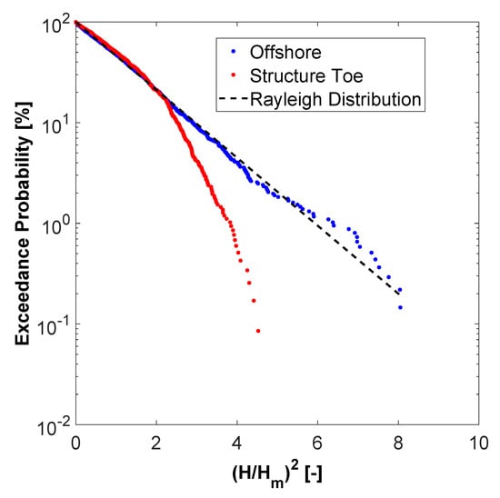
Figure 3.
Distribution of the measured incident wave heights for conditions generated by the wave paddle with comparison against expected Rayleigh Distribution.
The waves near the paddle closely match the Rayleigh distribution indicating that the paddle is indeed accurately reproducing a suitable sea state. The distribution at the structure toe shows a divergence from the Rayleigh distributions; this is caused by shoaling, triad interactions and depth-induced wave breaking. This agrees with the work of [31] which demonstrated a similar downward curved relation for the taller waves in shallow water like that present at the structure toe in this work. Further work showed these results to be consistent throughout the different wave conditions, and this additional analysis can be found in [32].
In addition, it was also important to check that the waves being generated matched the desired JONSWAP spectrum. The measure wave time series for each test was analysed in the frequency domain, and has been plotted in Figure 4, where f is the frequency and is the energy density function.
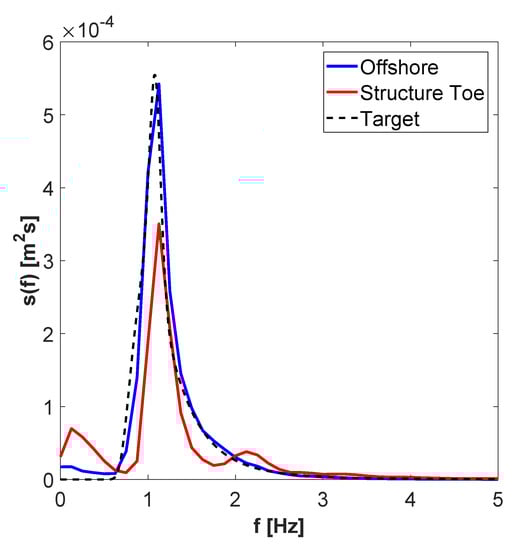
Figure 4.
Measured spectra at different locations in the wave flume for conditions generated by the wave paddle.
This figure shows that the offshore wave energy density closely matches the shape of the target JONSWAP spectrum for this wave condition, suggesting the paddle is accurately reproducing this spectrum. Like the wave height distribution, the spectrum transforms closer to the structure toe due to shoaling, wave breaking, and reflection from the structure itself. Similarly to the wave height distribution, further work showed these results to be consistent throughout the different wave conditions, and this additional analysis can be found in [32].
4. Results
4.1. Overtopping Discharge
First, we consider the variation in the overtopping discharge , for the 20 tests which were repeated using the exact same time series. The overtopping discharge was calculated for each test, with the results plotted using the dimensionless parameters, and in Figure 5, defined as and . Using the dimensionless values, it allows a direct comparison between the different tests.
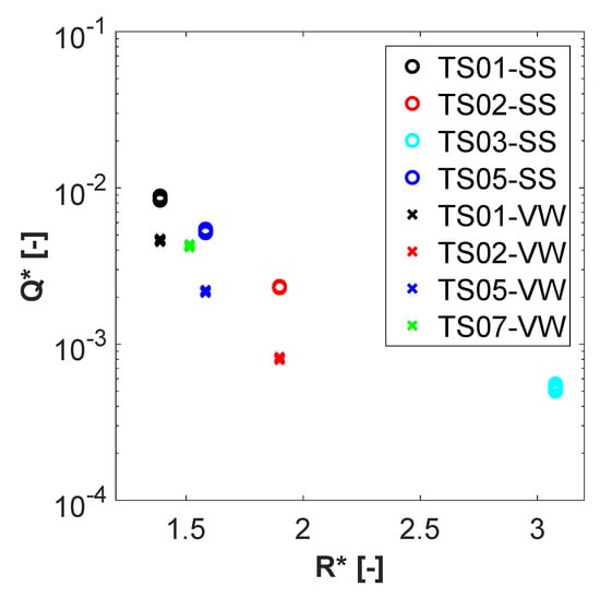
Figure 5.
Graph showing plotted against for each test conditions with identical offshore wave time series.
Figure 5 shows the results from both the smooth slope, and the vertical wall tests. It can be observed that there is some variation present in these nominally identical test runs. The magnitude of this variation remains fairly consistent across both the different levels of overtopping, and both structure types. To quantify this further, the variation in is calculated as a percentage difference for each test condition using the following formula:
where is the minimum value of the parameter of interest measured and is the maximum value measured. The results of this are shown in Table 2.
Table 2.
Percentage difference in and for non-random seeding tests.
The results observed here experience a level of variation that is significantly lower than the suggested in the work of [24] for both of the structure types, and for the different levels of overtopping. At this small scale, this level of variation is the equivalent to differences of less than a few millimetres in the depth detected in the tank, suggesting that at larger scales this variation would decrease further. The percentage difference in is also calculated here (see Table 2) to see if the variation measured is due to slight differences in the generated wave time series. The values for the percentage difference in were generally found to be less than those for the suggesting that the variation in does not purely originate from variation in but other laboratory effects.
Next, we examine the variation in the overtopping discharges based on the random seeding tests. To compare the variation in the prediction of overtopping from the physical model with that obtained when using empirical methods, the results were also compared with those calculated using formulae found within the latest version of [1]. Firstly, we examined the smooth slope structure, the most suitable formula for the conditions presented here has been developed from the work of [10]. The formula used is detailed below, or can be found as Equation in the latest version of [1], and calculates the predicted dimensionless overtopping for the structure:
where for and for , , with a maximum of and for and .
This equation gives the mean value approach for wave overtopping and for the design or safety assessment approach; one standard deviation should be added providing the confidence bounds of the formulae. For the two coefficients a and b, this means that one should take and , for a and b, where with being the mean and is the standard deviation, which is calculated as where N is the number of samples considered.
Results of the comparison are plotted in Figure 6.
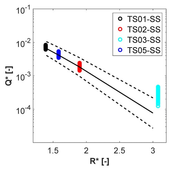
Figure 6.
Graph showing plotted against for random seeding test with smooth slope structure. Solid line: Empirical prediction. Dashed line: Confidence Bounds.
It can be observed here that the results from the physical model show very good agreement with those obtained using the empirical method, in all but the very lowest overtopping condition. The mismatch at the lower end of the results is most likely due to the calibration of the equation based on the work of [10]. This was based on structures with small relative freeboards, which is not the case for the lowest level of overtopping. One thing that can clearly be observed in these results is that, although there is variation in the prediction of overtopping in the physical model, it is well within the confidence bounds of the empirical method.
To compare the results from the vertical wall tests with the empirical methods, we must use a different formula. As no significant breaking was occurring in front of the vertical wall in the tests, we consider it to be in relatively deep water, where waves are not being significantly influenced by the sloping foreshore, we therefore used Equation 7.1 from [1], which is shown below:
The results from the vertical wall tests using the physical model and those calculated using the empirical prediction are plotted in Figure 7.
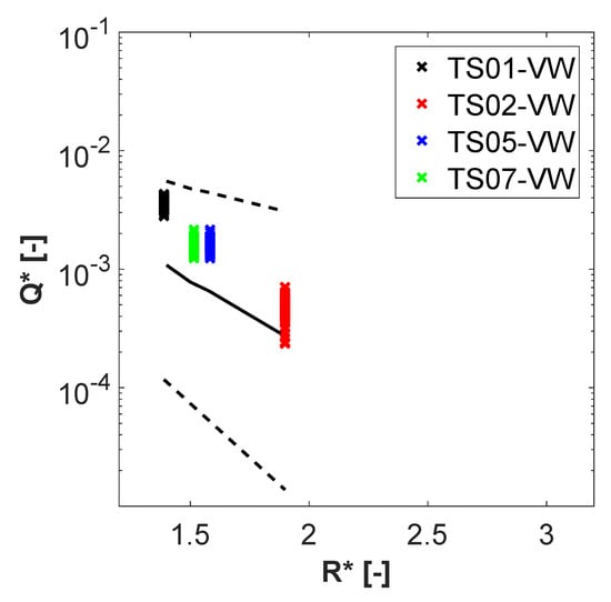
Figure 7.
Graph showing plotted against for random seeding test with vertical wall structure. Solid line: Empirical prediction. Dashed line: Confidence Bounds.
Similarly to the smooth slope tests, the results show good agreement with the empirical prediction, this time across all of the tests carried out. It is also clear that the variation in the measurement of overtopping using the physical model is still within the confidence bounds used for the empirical method. It can also be observed across both sets of tests that the variation in overtopping is clearly dependent on the level of overtopping that occurred, with variation being highest in lower overtopping conditions, generally found when the relative freeboard is larger.
Using the same method as for the non-random seeding tests, the percentage differences in have been calculated and can be seen in Table 3. The percentage difference calculated using the empirical formulae is also included in this table. There are three main points that should be acknowledged from these results. Firstly, it can clearly be observed here that, unlike in the non-random seeding tests, the variation in is highly dependent on the magnitude of overtopping occurring. The tests with smaller incoming wave conditions, or those based on the vertical wall, and therefore experienced lower levels of overtopping show larger variation than those that experienced higher levels of overtopping. The second point is that the magnitude of the variation, in terms of for the low overtopping tests, is shown to be up to . This is a significant difference in the prediction of the overtopping discharge from the same wave energy spectrum, suggesting that overtopping could be significantly under-predicted depending on the exact time series utilised. The third point is that, although relatively large variation is observed across the physical model tests, these are still a lot less than those incorporated via the confidence bounds into the empirical methods.
Table 3.
Percentage difference in and for random seeding tests.
Additionally, the percentage difference in has also been calculated, and can be found in Table 3. Although this variation shows slightly more variability than those for the non-random seeding tests, it is still significantly smaller than that found for . This suggests that some of the wave sequences produced by the paddle may not fit the wave statistics as closely as others, but does not significantly change the findings with regard to variability in .
4.2. Probability of Overtopping
It has been observed here that the variation in the overtopping discharge is related to the level of overtopping; therefore, analysis was carried out to quantify further whether the magnitude of variation in the discharge is directly related to the probability of overtopping for the physical model, as found in the analysis of numerical modelling prediction of overtopping in [25], which focussed solely on smooth slope structures.
The results from the physical model, with both types of structure, can be seen in Figure 8, where the probability of overtopping () is plotted against the overtopping discharge (q). is calculated by , where is the number of waves that overtopped the structure and is the total number of waves generated by the wave paddle in each test. was calculated using the peak detection method described earlier in this work, in order to identify each overtopping event, providing an approximation of the total number of events that occurred. was calculated by applying the zero-crossing method to the incoming waves measured at at the toe of the foreshore, identifying each individual wave, and therefore providing a value for the total number of waves in the test.
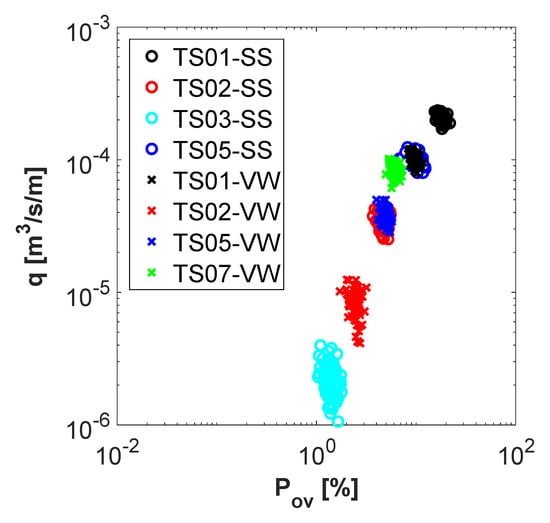
Figure 8.
Graph showing plotted against q for random seeding test with both structures.
These results show that the different types of structures appear to have no direct impact on the magnitude of the variation in q. This means that, where the magnitude of overtopping is similar, the level of variability is similar, irregardless of the shape of the structure or the incoming wave parameters, suggesting that is indeed the main influencing factor controlling variability.
4.3. Individual and Maximum Overtopping Volumes
Overtopping discharge and probability of overtopping are useful metrics in the design of coastal structures, but in terms of the safety of users and potential damage, the individual overtopping volumes are also important. There are two characteristics to be examined here, both the distributions of the individual overtopping volumes , and the maximum overtopping volume . As we have already found that variability is highly dependent on , the is considered with relation to this parameter and is plotted in Figure 9.
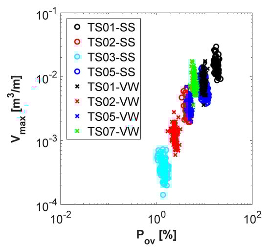
Figure 9.
Graph showing plotted against for a random seeding test with both structures.
Similarly to q, it can be seen that does show variation, but still only within one order of magnitude. There is a small increase in variation which is most likely due to the extreme nature of the value, as opposed to the average value of q, i.e., a single large volume has more influence when not averaged across all of the volumes. If we look at the variation in , it can also be seen that the value of has less influence on this variability with all the tests showing a similar level of variation for all the levels of overtopping.
To examine this further, the individual volume distributions are considered. Firstly, the empirical cumulative distribution functions of the individual overtopping volumes for each of the 100 random seeding tests for each wave condition with the smooth slope have been plotted in Figure 10. These have been normalised by dividing each individual volume measured, by the mean of the volumes measured for each test; this allows a direct comparison between the different levels of overtopping.
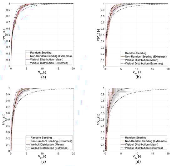
Figure 10.
Cumulative density functions showing distributions of individual overtopping volumes for smooth slope. (a) TS01-SS; (b) TS05-SS; (c) TS02-SS; (d) TS03-SS.
These graphs clearly show the increase in variation of these distributions of individual overtopping volumes due to the overall decrease in overtopping. The number of overtopping events can also be seen to decrease as the overall overtopping magnitude decreases, thus increasing the significance of each individual overtopping volumes in each time series.
The probability distribution of was investigated by a number of researchers ([10,11,33]) and found to generally follow a two parameter Weibull distribution:
where is the exceedance probability of each overtopping volume. The scale factor, a, and the shape factor, b, can vary depending on the exact empirical method chosen which is selected based on the conditions present. In this work, the distributions were fitted with an idealised Weibull distribution. These have been obtained by fitting the Weibull distribution to each individual time series, and then using the mean values calculated for the scale and shape parameters, along with the extreme values for the outer limits. As expected, the Weibull distribution shows a good match with the measured distributions across all of the levels of overtopping, albeit with differing values for shape and scale parameters.
Additionally, on these graphs, two distributions from the measured non-random seeding tests have been included. These represent the extremes of the measurements of for these tests. As expected from the earlier analysis, the variation in these is significantly lower than when random seeding is introduced. This is particularly noticeable in the lower overtopping tests, where the variation magnitude differs more.
Now, the individual volumes for the vertical wall are considered using the same method, resulting in Figure 11.
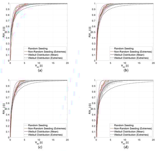
Figure 11.
Cumulative density functions showing distributions of individual overtopping volumes of vertical wall.(a) TS01-VW; (b) TS07-VW; (c) TS05-VW; (d) TS02-VW.
These graphs clearly show the same behaviour as those using the smooth slope structure; again, it can be seen that the variation increases with the decrease in overall overtopping magnitude. It has also been shown once again that this is not directly influenced by the type of structure, confirming that is the main parameter influencing the variability in overtopping prediction due to the random seeding of the offshore wave time series.
5. Discussion
The variability in the physical model in predicting q due to both different seeding and laboratory effects has been established. It is important to compare these two sets of results, so that the variabilities can be separated. This is carried out by calculating the relative standard deviation () in q for each of the tests. represents a standardised measure for the dispersion of a frequency distribution, and is calculated as the ratio of the standard deviation () to the mean () of the results (), in this case using the overtopping discharge. These are plotted against the relative freeboard in Figure 12 for both structures.
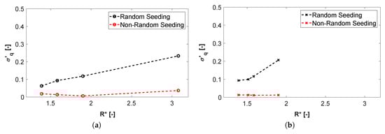
Figure 12.
of q for Random Seeding and Non-Random Seeding tests. (a) smooth slope; (b) vertical wall.
It can be seen on these graphs that for the non-random seeding remains fairly consistent throughout the different tests across both structural geometries, whereas the for the random seeding tests increases significantly as increases. There is a larger increase in observed at a lower value of for the vertical wall; this is due to the lower overtopping discharges, and subsequent greater variability experienced by the vertical wall than the smooth slope for the same wave conditions and crest height.
Across the two tested geometries, the value of for the non-random seeding equates to approximately . This suggests that, within the physical modelling of overtopping, there is always a very small amount of variation that can be equated simply to laboratory effects, and cannot easily be removed.
When the variation introduced due to random seeding is considered, results show that the magnitude of this is influenced by the magnitude of overtopping, i.e., the less overtopping, the higher the variation. This ranges from 6–25% in this work, and suggests that the small variation introduced due to laboratory effects is more significant in the tests with greater overtopping than those with small overtopping levels where the larger variation lowers the significance of this in the overall variability of the results.
In this work, a total of 100 random seeding tests have been carried out for each test condition. This is a large number of tests, and, in reality, it is not feasible to carry out this many repetitions; it was therefore decided to establish a more suitable value for the number of repetitions required. This was carried out by taking the full overtopping discharge calculated for each of the 100 tests and randomly sampling with different number of observations, namely 2, 5, 10, 20 and 50 samples. For each of these subsets of results, the values of were calculated, and analysed to see when the values of converged, suggesting that the minimum number of tests required had been met. When , it was found that a minimum of 20 repetitions was required; this could decrease to 10 repetitions when . This agrees with the findings of [28], which found that, when at least 20 tests provided a good estimate; this is the region where .
6. Conclusions
The paper quantifies the influence on wave overtopping of the initial random seeding on the generation of wave time series from wave energy spectra in a small scale physical model. Overall, the findings from these experiments agree with previous numerical investigations of the same phenomenon [25,26].
Although the experiments carried out in this work are on a small scale, the relative comparison of experiments within this dataset allows for quantifying the magnitude of the variability among and establishing a relationship with the probability of overtopping. The scale effects present in the experiment do not allow for extrapolate definitive conclusions valid at all scales but provide some guidelines for experiments in similar scales. Note that [14] reported that the majority of tests in the new wave overtopping database comes from tests with .
The results have also been compared with the most up-to-date formulae found in [1]. The variability found in the present results is lower than the overall variability in the formulae, with all results falling within the provided confidence bounds unless the conditions deviated from the exact criteria of the formulae used. However, the uncertainty introduced by iso-energetic sequences of waves is still significant. By using it is found that this variability is approximately between and of the , i.e., for , the variability could be comparable with . This indicates the need of taking this factor into account when experimental tests are performed, by ideally repeating tests in this region of to estimate the range of . The number of repetitions required has been found to be a minimum of 20 when , but this can decrease to 10 repetitions when is higher.
Author Contributions
This work was carried out as part of the PhD of H.E.W.; H.E.W. and R.B. planned the test campaign for this paper. The experimental tests and analysis were performed by H.E.W., with additional analysis from R.B. The original draft of the paper was written by H.E.W.; R.B., A.R. and N.D. performed a detailed review and editing of the draft paper and contributed with valuable suggestions. Supervision of the project was by R.B. and N.D. Funding acquisition was by R.B.
Funding
Hannah Williams and Riccardo Briganti were supported by the Engineering and Physical Sciences Research Council Career Acceleration Fellowship (EP/I004505/1).
Acknowledgments
The authors would also like to thank Steve Gange and Marco Matteucci at the University of Nottingham for their support during the experimental tests carried out in this work.
Conflicts of Interest
The authors declare no conflict of interest.
References
- Van der Meer, J.W.; Allsop, N.W.H.; Bruce, T.; De Rouck, J.; Kortenhaus, A.; Pullen, T.; Schüttrumpf, H.; Troch, P.; Zanuttigh, B. EurOtop 2018. Manual on Wave Overtopping of Sea Defences and Related Structures. An Overtopping Manual Largely Based on European Research, but for Worldwide Application; Environment Agency: Bristol, UK, 2018.
- Troch, P.; Geeraerts, J.; van de Walle, B.; De Rouck, J.; Van Damme, L.; Allsop, N.W.H.; Franco, L. Full-scale wave-overtopping measurements on the Zeebrugge rubble mound breakwater. Coast. Eng. 2004, 51, 609–628. [Google Scholar] [CrossRef]
- Briganti, R.; Bellotti, G.; Franco, L.; De Rouck, J.; Geeraerts, J. Field measurements of wave overtopping at the rubble mound breakwater of Rome Ostia yacht harbour. Coast. Eng. 2005, 52, 1155–1174. [Google Scholar] [CrossRef]
- Pullen, T.; Allsop, N.W.H.; Bruce, T.; Pearson, J. Field and laboratory measurements of mean overtopping discharges and spatial distributions at vertical seawalls. Coast. Eng. 2009, 56, 121–140. [Google Scholar] [CrossRef]
- Franco, L.; Geeraerts, J.; Briganti, R.; Willems, M.; Bellotti, G.; De Rouck, J. Prototype measurements and small-scale model tests of wave overtopping at shallow rubble-mound breakwaters: The Ostia-Rome yacht harbour case. Coast. Eng. 2009, 56, 154–165. [Google Scholar] [CrossRef]
- Pearson, J.; Bruce, T.; Allsop, N.W.H. Prediction of wave overtopping at steep seawalls—Variabilities and uncertainties. In Proceedings of the Fourth International Symposium on Ocean Wave Measurement and Analysis, San Francisco, CA, USA, 2–6 September 2001; Volume 1, pp. 1797–1808. [Google Scholar]
- Van Gent, M.R.A.; van den Boogaard, H.F.P.; Pozueta, B.; Medina, J.R. Neural network modelling of wave overtopping at coastal structures. Coast. Eng. 2007, 54, 586–593. [Google Scholar] [CrossRef]
- Reis, M.T.; Neves, M.G.; Hedges, T. Investigating the Lengths of Scale Model Tests to Determine Mean Wave Overtopping Discharges. Coast. Eng. J. 2008, 50, 441–462. [Google Scholar] [CrossRef]
- Bruce, T.; van der Meer, J.W.; Franco, L.; Pearson, J.M. Overtopping performance of different armour units for rubble mound breakwaters. Coast. Eng. 2009, 56, 166–179. [Google Scholar] [CrossRef]
- Victor, L.; van der Meer, J.W.; Troch, P. Probability distribution of individual wave overtopping volumes for smooth impermeable steep slopes with low crest freeboards. Coast. Eng. 2012, 64, 87–101. [Google Scholar] [CrossRef]
- Nørgaard, J.Q.H.; Lykke Andersen, T.; Burcharth, H.F. Distribution of individual wave overtopping volumes in shallow water wave conditions. Coast. Eng. 2014, 83, 15–23. [Google Scholar] [CrossRef]
- Van Doorslaer, K.; Romano, A.; De Rouck, J.; Kortenhaus, A. Impacts on a storm wall caused by non-breaking waves overtopping a smooth dike slope. Coast. Eng. 2017, 120, 93–111. [Google Scholar] [CrossRef]
- Martinelli, L.; Ruol, P.; Volpato, M.; Favaretto, C.; Castellino, M.; De Girolamo, P.; Franco, L.; Romano, A.; Sammarco, P. Experimental investigation on non-breaking wave forces and overtopping at the recurved parapets of vertical breakwaters. Coast. Eng. 2018, 141, 52–67. [Google Scholar] [CrossRef]
- Van der Meer, J.W.; Verhaeghe, H.; Steendam, G.J. The new wave overtopping database for coastal structures. Coast. Eng. 2009, 56, 108–120. [Google Scholar] [CrossRef]
- Dodd, N. A numerical model of wave run-up, overtopping and regeneration. J. Waterw. Port Coast. Ocean Eng. 1998, 124, 73–81. [Google Scholar] [CrossRef]
- Hubbard, M.E.; Dodd, N. A 2-d numerical model of wave run-up and overtopping. Coast. Eng. 2002, 47, 1–26. [Google Scholar] [CrossRef]
- Reeve, D.E.; Soliman, A.; Lin, P.Z. Numerical study of combined overflow and wave overtopping over a smooth impremeable seawall. Coast. Eng. 2008, 55, 155–166. [Google Scholar] [CrossRef]
- Ingram, D.M.; Gao, F.; Causon, D.M.; Mingham, C.G.; Troch, P. Numerical investigations of wave overtopping at coastal structures. Coast. Eng. 2009, 56, 190–202. [Google Scholar] [CrossRef]
- Tonelli, M.; Petti, M. Numerical simulation of wave overtopping at coastal dukes and low-crested structures by means of a shock-capturing Boussinesq model. Coast. Eng. 2013, 79, 75–88. [Google Scholar] [CrossRef]
- Suzuki, T.; Altomare, C.; Veale, W.; Verwaest, T.; Trouw, K.; Troch, P.; Zijlema, M. Efficent and robust wave overtopping estimation for impermeable coastal structures in shallow foreshores using SWASH. Coast. Eng. 2017, 122, 108–123. [Google Scholar] [CrossRef]
- Akbari, H. Simulation of wave overtopping using an improved SPH method. Coast. Eng. 2017, 126, 51–68. [Google Scholar] [CrossRef]
- Castellino, M.; Sammarco, P.; Romano, A.; Martinelli, L.; Ruol, P.; Franco, L.; De Girolamo, P. Large impulsive forces on recurved parapets under non-breaking waves. A numerical study. Coast. Eng. 2018, 136, 1–15. [Google Scholar] [CrossRef]
- McCabe, M.V.; Stansby, P.K.; Apsley, D.D. Coupled wave action and shallow-water modelling for random wave runup on a slope. J. Hydraul. Res. 2011, 49, 512–522. [Google Scholar] [CrossRef]
- McCabe, M.V.; Stansby, P.K.; Apsley, D.D. Random wave runup and overtopping a steep sea wall: Shallow-water and Boussinesq modelling with generalised breaking and wall impact algorithms validated against laboratory and field measurements. Coast. Eng. 2013, 74, 33–49. [Google Scholar] [CrossRef]
- Williams, H.E.; Briganti, R.; Pullen, T. The role of offshore boundary conditions in the uncertainty of numerical prediction of wave overtopping using nonlinear shallow water Equations. Coast. Eng. 2014, 89, 30–44. [Google Scholar] [CrossRef]
- Williams, H.E.; Briganti, R.; Pullen, T.; Dodd, N. The Uncertainty in the Prediction of the Distribution of Individual Wave Overtopping Volumes Using a Nonlinear Shallow Water Equation Solver. J. Coast. Res. 2016, 32, 946–953. [Google Scholar] [CrossRef]
- Palemón-Arcos, L.; Torres-Freyermuth, A.; Pedrozo-Acuña, A.; Salles, P. On the role of uncertainty for the study of wave–structure interaction. Coast. Eng. 2015, 106, 32–41. [Google Scholar] [CrossRef]
- Romano, A.; Bellotti, G.; Briganti, R.; Franco, L. Uncertainties in the physical modelling of the wave overtopping over a rubble mound breakwater: The role of the seeding number and of the test duration. Coast. Eng. 2015, 103, 15–21. [Google Scholar] [CrossRef]
- Hughes, S. Physical Models and Laboratory Techniques in Coastal Engineering; World Scientific: New York, NY, USA, 1993. [Google Scholar]
- Longuet-Higgins, M.S. On the statistical distribution of the heights of sea waves. J. Mar. Res. 1952, 9, 245–266. [Google Scholar]
- Battjes, J.A.; Groenendijk, H.W. Wave height distributions on shallow foreshores. Coast. Eng. 2000, 40, 161–182. [Google Scholar] [CrossRef]
- Williams, H.E. Uncertainty in the Prediction of Overtopping Parameters in Numerical and Physical Models due to Offshore Spectral Boundary Conditions. Ph.D. Thesis, University of Nottingham, Nottingham, UK, 2015. [Google Scholar]
- Van der Meer, J.; Janssen, J. Wave Run-Up and Wave Overtopping at Dikes and Revetments; Delft Hydraulics: Delft, The Netherlands, 1994. [Google Scholar]
© 2019 by the authors. Licensee MDPI, Basel, Switzerland. This article is an open access article distributed under the terms and conditions of the Creative Commons Attribution (CC BY) license (http://creativecommons.org/licenses/by/4.0/).