Article

Wave Climate Change in the North Sea and Baltic Sea

by
Antonio Bonaduce
1,*,
Joanna Staneva
1,*,
Arno Behrens
1,
Jean-Raymond Bidlot
2 and
Renate Anna Irma Wilcke
3
1
Helmholtz-Zentrum Geesthacht Centre for Materials and Coastal Research (HZG), 21502 Geesthacht, Germany
2
European Centre for Medium-range Weather Forecasts (ECMWF), Reading RG2 9AX, UK
3
Swedish Meteorological and Hydrological Institute (SMHI), SE-601 76 Norrkoping, Sweden
*
Authors to whom correspondence should be addressed.
J. Mar. Sci. Eng. 2019, 7(6), 166; https://doi.org/10.3390/jmse7060166
Submission received: 16 April 2019 / Revised: 9 May 2019 / Accepted: 27 May 2019 / Published: 30 May 2019

Abstract

:
Wave climate change by the end of the 21st century (2075–2100) was investigated using a regional wave climate projection under the RCP 8.5 scenario. The performance of the historical run (1980–2005) in representing the present wave climate was assessed when compared with in situ (e.g., GTS) and remote sensing (i.e., Jason-1) observations and wave hindcasts (e.g., ERA5-hindcast). Compared with significant wave height observations in different subdomains, errors on the order of 20–30% were observed. A Principal Component (PC) analysis showed that the temporal leading modes obtained from in situ data were well correlated (0.9) with those from the historical run. Despite systematic differences (10%), the general features of the present wave climate were captured by the historical run. In the future climate projection, with respect to the historical run, similar wave climate change patterns were observed when considering both the mean and severe wave conditions, which were generally larger during summer. The range of variation in the projected extremes (±10%) was consistent with those observed in previous studies both at the global and regional spatial scales. The most interesting feature was the projected increase in extreme wind speed, surface Stokes drift speed and significant wave height in the Northeast Atlantic. On the other hand, a decrease was observed in the North Sea and the southern part of the Baltic Sea basin, while increased extreme values occurred in the Gulf of Bothnia during winter.

1. Introduction

Ocean wind-generated waves (i.e., surface gravity waves) are an important component of Earth’s climate system, as they contribute to modulate the interaction between the ocean and the atmosphere in terms of mass, heat, and momentum (e.g., [1,2]). Waves integrate the effect of winds over the fetch across which they blow [3], which can be influenced by changes in sea ice extent [4] (e.g., sea ice retreat due to global warming). Depending on their degree of coupling with the atmosphere, waves are typically defined as wind sea waves, which receive momentum directly from wind, or swell waves, which are mature waves with long wavelengths that can propagate far away from their generation source across entire ocean basins (e.g., [5]). As a consequence, a change in winds (e.g., speed and direction) at the local scale can affect the wave climate variability elsewhere in the global ocean due to wave propagation characteristics. The focus of this study is to investigate the projected changes in the regional wave climates of the North Sea, Northeast Atlantic, and Baltic Sea (integrated into one model system) toward the end of the 21st century and to assess the historical climate simulation against the newly available wave hindcasts. The Fifth Assessment Report (AR5) of the Intergovernmental Panel on Climate Change (IPCC; [6]) iterated that because wind waves integrate atmospheric dynamics characteristics, they can be considered as a potential indicator of climate variability and change in oceans [7] and recognized that ocean waves are one of the main drivers of coastal hazards (e.g., coastal erosion and inundation) in combination with sea-level rise due to ocean mass variations and thermal expansion [8]. As part of Earth’s climate system, where dominant and subdominant processes modulate their reciprocal responses through multiple feedbacks [9], ocean waves show complex response patterns to climate change. The increase in temperature observed in the ocean and atmosphere during the last century [6] will likely persist during the 21st century, which will be mainly due to the increase in greenhouse gas emissions, and will lead to changes in surface wind speeds, which will affect the future wave climate [10]. The IPCC AR5 strictly relies on the Coupled Model Intercomparison Experiment Project Phase 5 (CMIP5; [11]), which includes projections of climate change driven by emission scenarios defined as representative concentration pathways (RCPs; [12]). RCPs are mitigation scenarios that, in contrast with the IPCC Special Report on Emissions Scenarios (SRES; [13]), assume that intervention policy on climate change will be adopted. Four RCPs were formulated in CMIP5, accounting for low (RCP2.6), intermediate (RCP4.5 and RCP6) and high (RCP8.5) emissions scenarios. RCP8.5 assumes a constant positive emission trend given by radiative forcing of 8.5 W m 2 by the end of the 21st century. Under this scenario, the global mean sea-level and surface temperatures at the end of the 21st century show anomalies relative to the period 1986–2005 in ranges from 0.45 m to 0.82 m and from 2.6 C to 4.8 C, respectively [6]. Following the approach proposed by several recent studies (e.g., [2,5,10,14]), the RCP8.5 scenario was selected in this study to investigate the maximum range of variations in the wave climate at the regional scale.
During past years, atmospheric forcings from the CMIP5 have been used to investigate future wave climate scenarios at the global scale by adopting a single-model (e.g., [5,10,15]) and multimodel (e.g., [1,16,17]) ensemble approach. At the regional scale, fewer studies have appeared in recent literature. Ref. [18], who used two radiative forcing scenarios (RCP 4.5 and RCP 8.5) to assess future wave conditions in the eastern North Pacific, observed decreasing mean and severe wave conditions. Ref. [19], who investigated the changes in significant wave heights toward the end of the 21st century, used the wind fields from the ensemble members of six different CMIP5 models to force a wave model (i.e., the wave ocean model (WAM)) that was implemented in the North Atlantic and observed decreases in wind speed and associated wave height in the region. Ref. [20] used ten different combinations of IPCC SRES to estimate the change in wave conditions towards the end of the 21st century in the North Sea and found an increase in mean and extreme wave heights in the eastern parts of the North Sea and a decrease in these heights in the western part of the basin in most of the projections. Ref. [21], who used two IPCC SRES (A1B and B1) to force the WAM wave model implemented in the Baltic Sea, observed coherent patterns of increased mean wave heights among the different simulations, which was not the case when considering the extremes.
These studies focused separately on the change in the wave climate in different basins (e.g., the North and Baltic Seas) by considering a spatial resolution (50 km; e.g., [19]) that could be not suitable to resolve high-gradient wave conditions [22] at the regional and subregional scales. In this study, we use a single model run under high emission scenario RCP8.5 to investigate the projected future wave climate in the North Sea, Northeast Atlantic, and Baltic Sea, which are considered to be connected basins, to obtain a consistent characterization of the wave climate in the regional domain resolved at a fine spatial resolution (5 km).
The specific objective is to assess the skill of historical regional wave climate simulation and use it as a reference to evaluate the wave climate projection by the end of the 21st century. The paper is organized as follows. Section 2 describes the wave model configuration used in this study, the experimental setup designed to assess the wave climate change toward the end of the century and the datasets used to validate the wave climate simulation during a historical period (1980–2005). The skill of the wave climate simulation used in this study is investigated in Section 3 by comparing the results with the observations and wave hindcasts during the historical period. The wave climate change projection (2075–2100) and how it compares with the present climate is discussed in Section 4. The results are summarized in Section 5, and some conclusions are drawn.

2. Wave Model Configuration and Experimental Design

In this study, the spectral wave model WAM was used. The WAM is a third-generation wave model that solves the wave transport equation explicitly without any presumptions on the shape of the wave spectrum. This model represents the physics of the wave evolution in accordance with our current knowledge for the full set of degrees of freedom in a 2D wave spectrum. A full description is given by [23,24,25,26]. In this application, the WAM Cycle 4.5.4 runs in shallow water mode, including bottom induced wave breaking on a model grid situated between 48 N to 66 N and −9 W to 31 E, with a spatial distribution of Δ ϕ Δ λ = 0.05 ∗ 0.1 (∼5 km) [27]. The 2-D wave spectra are calculated for 24 directional bands at 15 each, starting at 7.5 , and measured clockwise with respect to true north, and 25 frequencies are logarithmically spaced from 0.042 Hz to 0.41 Hz at intervals of Δ f / f = 0.1. At its open boundaries, the regional wave model uses the full two-dimensional spectral information provided by a global wave model (spatial resolution of 1 ∗ 1 ). The underlying bathymetry is based on the one-minute global General Bathymetric Chart of the Oceans (GEBCO) topography (Figure 1). The results of the regional wave model are stored every hour. The driving forces are the forecasted wind fields at 10 m above the surface (U10; 3-hourly) delivered by the most recent version of the Rossby Center regional atmospheric model (RCA4; [28]), which runs on a 12.5 km grid and is driven along its boundaries with data from the European Community Earth-System Model (EC-EARTH) ([29,30]; www.ec-earth.org). The EC-Earth general circulation model is a fully coupled atmosphere-ocean-sea ice system [31,32]. Ice cover in our simulations has been considered and was also taken from the EC-Earth data.
To investigate the regional wave climate change, two periods of 25 years were used (the first is a historical period (1980–2005), which is referred to as “historical”, and the second is the “future” period toward the end of the 21st century (2075–2100)) under high-emission scenario (RCP8.5), which corresponds to a positive perturbation in the radiative budget at the top of the atmosphere of 8.5 W m 2 at 2100. A 25-year historical period, which is representative of the present climate, was selected in reference to the temporal window used by [5], and a 25-year period by the end of the 21st century was selected accordingly. To assess the skill of the wave model in reproducing the present wave climate, the historical run was compared with the available in situ and remote sensing data, the European Centre for Medium-range Weather Forecasts (ECMWF) Re-analysis data (ERA5; [33]) and the Norwegian Reanalysis Archive (NORA10; [34]) wave hindcasts, as described in the following sections. The future climate projection was then compared with the historical integration to assess the reliability of wave climate change.

2.1. Observation Datasets

The historical run was first compared with in situ data at the observation positions, as shown in Figure 1 (red dots). The data were obtained from the Global Telecommunication System (GTS) and from the Copernicus Marine Environment Service (CMEMS) in situ Thematic Centre (INS TAC). GTS data are obtained by and archived at the ECMWF ([35]). Other data were gathered by the ECMWF as part of the Joint Technical Commission for Oceanography and Marine Meteorology (JCOMM) wave forecast verification project [36]. In situ data in the Baltic Sea were obtained from the CMEMS INS TAC, which collects near-real-time data from the Baltic Operational Oceanographic System (BOOS) members. Data are continuously updated and quality controlled, as documented at CMEMS INS-TAC (http://marine.copernicus.eu/documents/QUID/CMEMS-INS-QUID-013-030-036.pdf), which also describes how to freely access the data (http://marine.copernicus.eu/documents/PUM/CMEMS-INS-PUM-013.pdf).
The historical run was also compared with remote sensing data on the significant wave height. The data used are produced by Deutsches Geodatisches Forschungsinstitut (DGFI) research institute of the Technische Universitat Munchen (TUM), where the altimetric waveforms are retracked to obtain reliable data both in the open ocean and in coastal areas [37,38], and are distributed via OpenADB (https://openadb.dgfi.tum.de). The dataset was selected to retrieve information from remote sensing data suitable for the open ocean (e.g., Northeast Atlantic), enclosed basins (e.g., Baltic Sea) and coastal areas considered in the wave climate simulation. The quality of the dataset over coastal areas (i.e., the German Bight) was described by [38], who analyzed significant wave height signals from Envisat, Jason-1 and Jason-2. Here, we used along-track data from Jason-1 (black lines in Figure 1), which is the only satellite mission in the DGFI-TUM dataset that has a lifetime (2002–2012) that overlaps the period spanned by the historical run over a relatively short temporal window (from 2002 to 2005).

2.2. Wave Hindcasts

In order to estimate the skill of the wave climate simulation at the regional scale, the historical run was compared with the ERA5 and NORA10 wave hindcasts. The NORA10 wave hindcast (hereafter referred as NORA-h) is a dynamical downscaling of the global ECMWF reanalysis (ERA-40; [39]), including the North Sea and the Norwegian Continental Shelf (NCS) [34,40] and represents a valuable dataset for wave climate studies (e.g., [41]) and validation of wave climate simulations e.g., [19]). Waves are generated using a different version of the WAM used in this study for simulating the wave climate and ran on a rotated longitude/latitude grid, which consists of a coarse 50-km resolution model forced by the ERA-40 wind fields and a nested 10 km resolution model forced by the High Resolution Limited Area Model (HIRLAM; [42]) winds. The NORA-h outputs are representative of hourly averaged data and are available every 3 h [43].
ERA5 is the fifth generation ECMWF atmospheric reanalysis of the global climate. The ERA5 reanalysis [33] is the successor of the ERA-Interim reanalysis [44], which provides data at finer spatial (31 km) and temporal (1 h) resolutions with respect to its predecessor. The ECMWF reanalysis ERA5 was produced using 4D-Var data assimilation with CY41R2 of ECMWF’s Integrated Forecast System (IFS), with 137 hybrid sigma/pressure (model) levels in the vertical direction, where the top level is 0.01 hPa [45]. As noted by [46], the temporal resolution of ERA5 is particularly relevant for wave model simulations at the regional scale, which was also considered in this study. Even though ERA5 wave data are already a major improvement with respect to ERA-Interim data [47], a more recent version (CY46R1) of the ECMWF wave model [45] has been used to produce a long hindcast. This latest hindcast was found to be of even better quality than ERA5 [48]. This hindcast is a wave model standalone (i.e., not coupled) run forced by ERA5 hourly 10 m neutral winds, surface air density, gustiness and sea ice cover. It uses different wave physics for the wind input and dissipation (ERA5: [49]; ERA5 hindcast: [50]). No wave data assimilation was performed, as was the case for ERA5 with all available spaceborne altimeter wave height data. The spatial and spectral resolutions were increased (ERA5 = 40 km, 24 directions, 30 frequencies; ERA5 hindcast = 14 km, 36 directions, 36 frequencies), and it was based on a more recent global bathymetry dataset (ERA5: ETOPO2; ERA5 hindcast: ETOPO1). Here, we used the ERA5 hindcast (hereafter referred as ERA5-h; Jean-Raymond Bidlot personal communication) hourly outputs to compare the historical run with the ECMWF ocean wave model output parameters [51] at the same temporal resolution.

3. Wave Climate Simulation over the Historical Period (1980–2005)

In this section, we compare the historical run with the available in situ and remote-sensing observations and with the ERA5 and NORA10 hindcasts to assess the accuracy of the numerical simulation in the past, which is used as a reference to understand the reliability of the future scenario projections. Compared with the observations, the skill of ERA5-h, both in terms of temporal variability and leading modes, is always higher than those of the other datasets. When comparing ERA5 with the in situ wave height observations from 2000 to 2018 (January), Ref. [47] observed a much improved quality in the ocean-wave analysis with respect to ERA-Interim over the same period. Ref. [46] compared ERA5 and remote-sensing data in the North Atlantic, North Sea and the Baltic Sea over a much shorter period based on Sentinel-3A data availability and observed a high synergy between the two data sources.
The results obtained in this study, to the best of our knowledge, represent a first assessment of the accuracy of ERA5-h data over a period longer than two decades. In the following part of this section, we present only the results of the comparison of the observations, ERA5-h and historical run. These results, as well as those obtained considering NORA10-h, are summarized in Table 1 and Table 2.

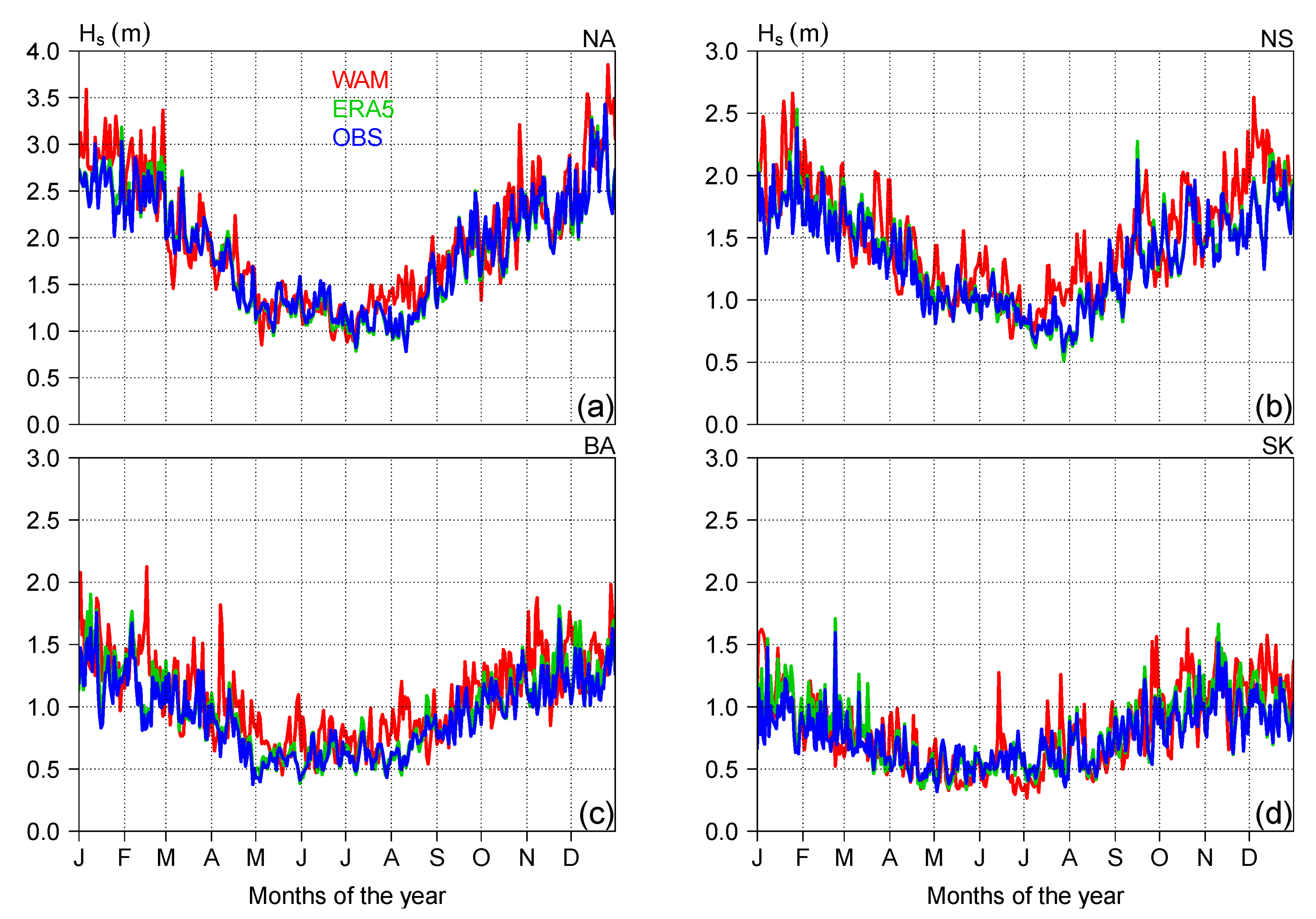
3.1. Validation at the Observation Positions

First, the historical run was validated by comparing it with in situ observations. The skill of the historical run was assessed over both the whole spatial domain (ALL) and over different subregions (Figure 1), such as in the Northeast Atlantic (NA), North Sea (NS), Skagerrak and Kattegat areas (SK) and Baltic Sea (BA). Following the approach proposed by [5], the collocated (at the observation positions) daily averages significant wave height ( H s ) obtained from the in situ observations, ERA5-h and historical run plotted in a Julian year are shown in Figure 2. The intra-annual variability was well captured in the historical run both at the regional and subregional scales (Figure 2 and Figure 3). At the regional scale, the agreement between the observations and ERA5-h is evident during all months of the year, with a relatively small positive bias during the periods from January to March and from September to December and a root mean square error (RMSE) that was approximately 8% of the mean wave height in the observation records (i.e., normalized RMSE, or NRMSE, in Table 1). A larger bias was observed considering the historical run over the same months of the year, as well as during summer (from July to September), when the highest agreement with the observations was observed considering ERA5-h; the NRMSE was larger than 20% considering all months of the year (Figure 2).
Similar results were also observed in the different subregions considered. During the last months of the year (from September to December), when wave heights started to increase in the Northeast Atlantic, the agreement among the observations, historical run and ERA5-h was the highest. This is also the subregion where the H s was the largest and where the numerical wave models performed better (showing the lowest NRMSE values) when both considering ERA5-h (∼3%) and the historical run (∼18%). Larger NRSME values (25%) were observed in the North Sea when looking at the historical run from July to August and from November to December, while ERA5-h always accurately reproduced the intra-annual variability in this area. In the SK and BA subregions, the wave heights were significantly lower than those in the Northeast Atlantic and the North Sea, and the numerical wave models showed lower accuracy in reproducing the wave heights in these areas. Moving towards the Danish straits, the SK represents a transition area between the Northwestern Shelf and the Baltic Sea, which is characterized by strong mass and energy transports that make these areas particularly interesting from ocean dynamics and sea state variability perspectives and challenging from a modelling perspective. In these areas, the accuracies of ERA5-h and the historical run were the lowest observed over the spatial domain (Figure 3, bottom right panel) due to discrepancies observed in the period from January to March (ERA5-h) and September to November (historical run). In the Baltic Sea, discrepancies between the observations and the historical run (31%) can be observed during all months of the year, while the ERA5-h was significantly more reliable (8%), which was probably due to the impact of the atmospheric observations assimilated during the reanalysis integration [46].
The accuracy of the historical run with respect to the in situ observations was also assessed in terms of temporal leading modes of variability by performing a principal component (PC) analysis, as shown in Figure 4 and Table 2. In the figure, the top panels show the two leading PCs obtained considering the ALL domain. In general, a good similarity between the portion of variance given by the observation PCs and those obtained in ERA5-h and the historical run was observed. The first PC (PC1) explained more than 45% of the variance in the H s signals given by in situ observations, which is representative of the H s annual cycle in the study area. The agreement between PC1 from the observations and ERA5-h (Figure 4, top left panel) is almost ideal and, despite small discrepancies, also well correlated with the historical run (0.9) at this temporal scale (Table 2). The second PC (PC2) is representative of the intra-annual variability and accounts for the 10% of the variance in the observed records. In the case of ERA5-h, the results observed considering PC1 can be extended to the comparison of PC2, while the historical run showed a lower accuracy (C = 0.5) over these shorter scales of variability, which was probably due to inaccuracies in the forcings used in the wave climate simulation. A PC analysis was also performed in the different subregions considered, as shown in the bottom panels of Figure 4. The ERA5-h PCs were ideally correlated with those of the observations, showing the impact of assimilating atmospheric data during ERA5-h integration (except in the SK and BA subregions). These are the subregions where the historical run and observation PCs were also not well correlated, except when considering PC1 in the Baltic Sea (0.7) (not shown). In the NA subregion, the two leading PCs of the historical run showed a good agreement with the observations, while this was not the case considering PC2 in the NS subregion (Figure 4, central right panel) due to discrepancies during the period from February to April.
The historical run was also validated using significant wave heights from the remote sensing data [37,38] of Jason-1 over the period from 2002 to 2005 (Figure 5), which overlaps the historical run and satellite mission data availability. The results confirmed those obtained when compared with in situ data, showing a good agreement between the historical run and satellite data in the North Atlantic and the North Sea (NRMSE < 30% ), with larger errors at the Danish Straits (SK subdomain) and in the Baltic Sea.

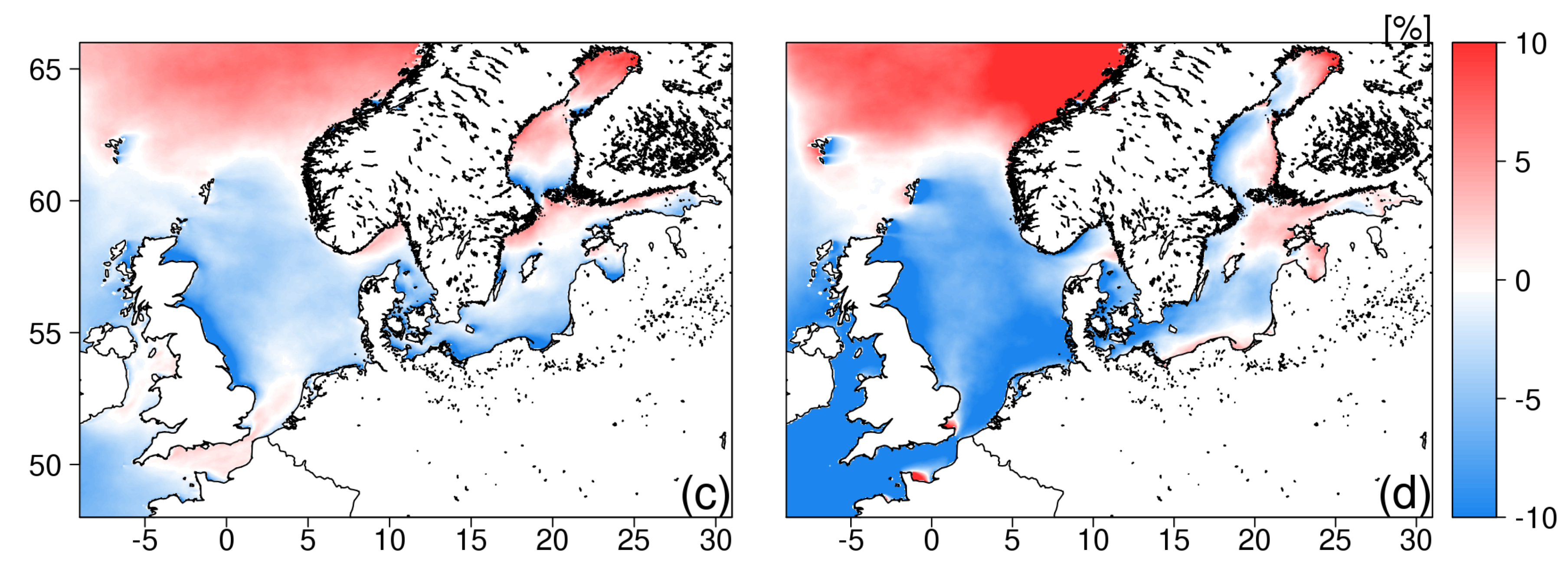
3.2. Validation over the Regional Domains

To obtain an estimate of the accuracy of the wave model over the whole spatial domain, the historical run was compared with the ERA5 and NORA10 hindcasts. In particular, we focused on the representation of the extremes in the different datasets to obtain a reference for the accuracy of the historical run and to use it to assess the reliability of the extremes observed in the future run. Following the approach used in the literature by [5,52], the top panels in Figure 6 show the relative difference between the historical run and ERA5 data-sets when considering the annual 95th percentile of 10 m wind speed (ERA5) and H s (ERA5-h) during winter (DJF) and summer (JJA). Here, the relative difference ( R D h ) is defined as:
R D h = R e f W A M R e f 100
where R e f is the reference dataset chosen to assess the skill of the historical run W A M . Positive (negative) values of R D h mean that the signals in the reference dataset are larger (smaller) than those in the historical run. The historical run evidently tends to overestimate the extremes values in the ERA5-hindcast by more than 10%, which is almost independent of the area and season considered.
Higher accuracy can be noticed when looking at wind speed during winter in the Northeast Atlantic and Baltic Sea, where R D h values smaller than 5% were also observed in summer. Looking at H s , small R D h values were observed only in the areas of the Northeast Atlantic characterized by the largest wave heights during winter. These results were partially confirmed comparing them with the NORA10-h results (Figure 6 bottom panels). During DJF, the historical run exceeded NORA10-h by less than 10% in the North Sea, while the opposite condition was observed in the North-Atlantic over the shelf areas along the UK coasts and in the Baltic Sea (due to the effect of meridional winds during this season). Positive differences were also observed during JJA in the Danish Straits and the southern part of the Baltic Sea. As in ERA5-h, the differences observed considering H s reflect those in wind speed also in NORA10-h (not shown).
An empirical orthogonal function (EOF) analysis [53,54] was performed to investigate how the spatial leading modes in the historical run compare with those of ERA5-h. Figure 7 shows the spatial patterns of the first EOF during winter (EOF1 DJF) and summer (EOF1 JJA), which were obtained by considering the monthly averaged H s . In the figure, the spatial leading modes show coherent patterns of variability between the datasets. EOF1 DJF represents almost 60% of the variance and accounts for large-scale H s seasonal variability. As expected, a smaller portion of variability (approximately 40%) was represented by EOF1 during summer (EOF1 JJA, Table 3). On the other hand, it is interesting to notice that in both datasets, EOF1 DJF and EOF1 JJA explain more than the 75% and 85%, respectively, of the variance in the Northeast Atlantic, North Sea and SK subregions, as the wave heights in these areas are dominated by the effects of seasonal winds (Table 3). At the regional scale, the maximum variance is found in the area of maximum significant wave height in the Northeast Atlantic and in the northern part of the North Sea. The largest differences were observed in the Baltic Sea. In this subregion, EOF1 DJF in ERA5-h clearly shows the influence of zonal and meridional winds in the southern part of the basin, which was also well depicted in the historical run. On the other hand, compared with EOF1 DJF, the summer EOF1 of ERA5-h showed a more uniform pattern of variability across the Baltic Sea basin, which was not well captured in the WAM historical run. EOF2 (Figure 8) represented more than 15% of total the variance in the signal in ERA5-h in DJF (Table 3) and more than 20% in JJA. The maximum variance values were observed in the Northeast Atlantic both in DJF and JJA. The main differences with the leading modes obtained in the historical run can be noticed during DJF and JJA in the northern part of the North Sea (at the separation between the continental slope and shelf) and during JJA in the Baltic Sea, which was probably due to the effect of meridional winds.
The results of the EOF analysis when considering H s can be extended to the leading modes of the surface Stokes drift speed (not shown). Table 3 and Table 4 summarize the results of the EOF analysis in terms of the variance represented by the first two leading modes obtained considering H s and surface Stokes drift, respectively, both at the regional scale and in the different subregions considered in this study. The description of the results of the EOF analysis when considering H s in the future run (Figure 9), is given in Section 4.
The results observed considering annual 95th percentiles were confirmed by comparing the average historical wave climate integration with ERA5-h (Figure A1 and Figure A2). From what was found for severe wave climate conditions, small departures (less than 5%) were observed when considering the 10 m wind speed and significant wave heights in the Northeast Atlantic during DJF. Larger differences were observed when considering average significant wave heights in the Baltic Sea during DJF, which were associated with local changes in the mean wave period (Figure A2, panels a and c).
Despite the differences between the two wave climate integrations, the general features of the present wave climate are captured by the historical run. The differences are mainly driven by discrepancies in the wind fields. Other discrepancies can be found in the physical and topographic features resolved by the models, as ERA5-h accounts for the latest wave physics of [50] and considers a subgrid scheme to resolve issues with islands (e.g., [2]). These final aspects are expected to have the same influence on future climate integration.

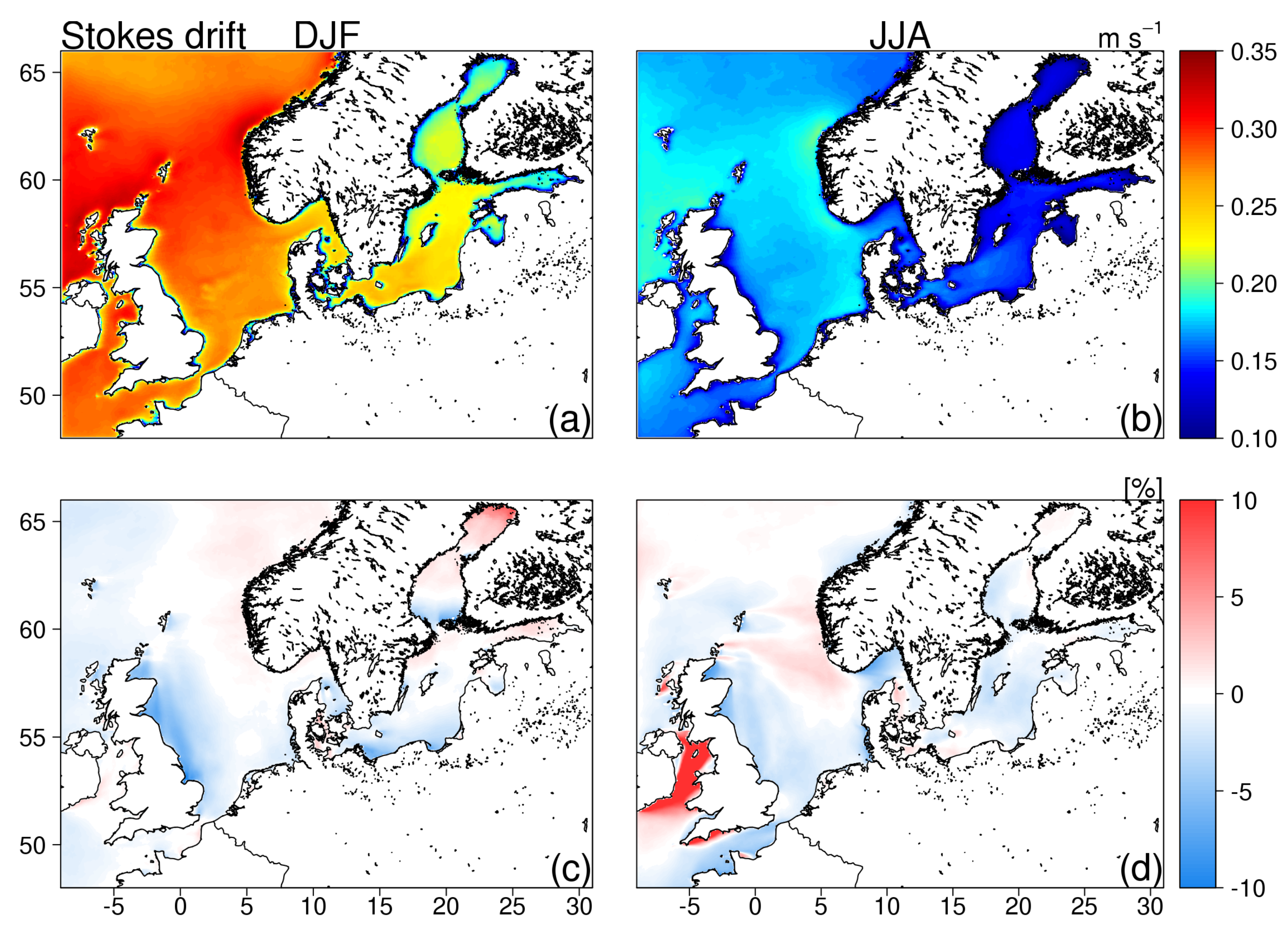
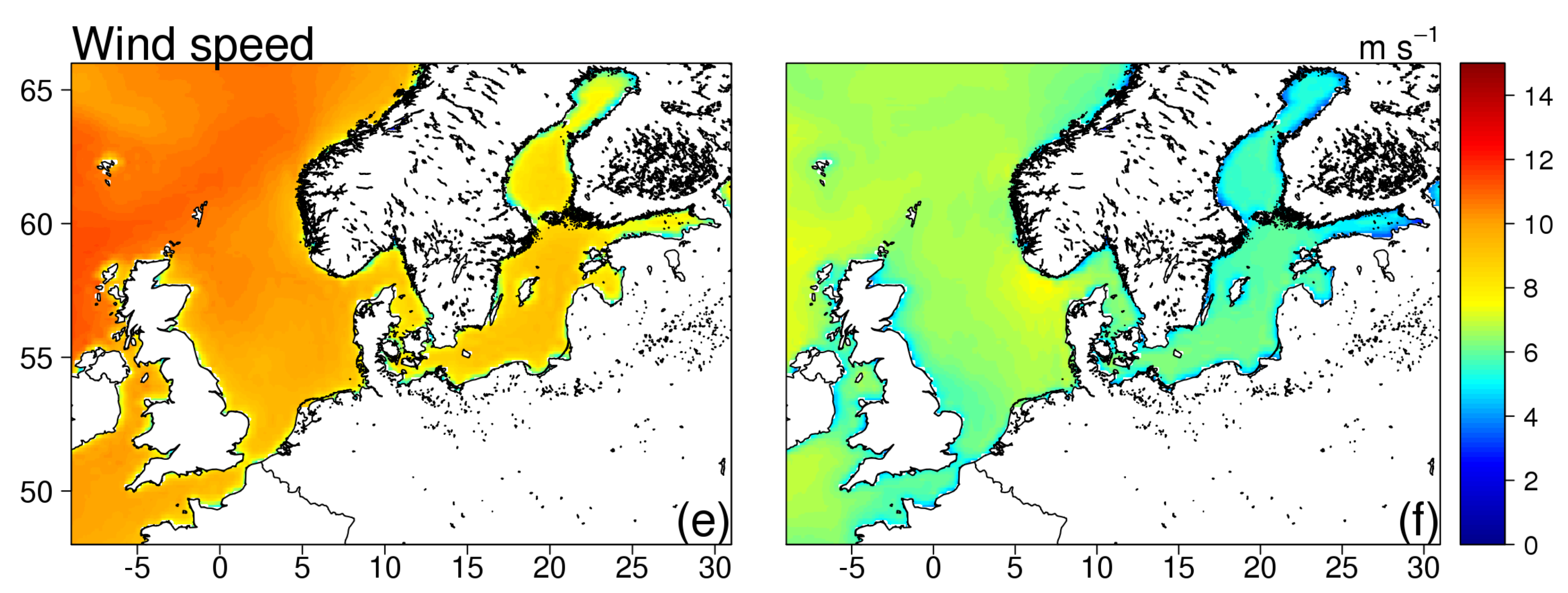
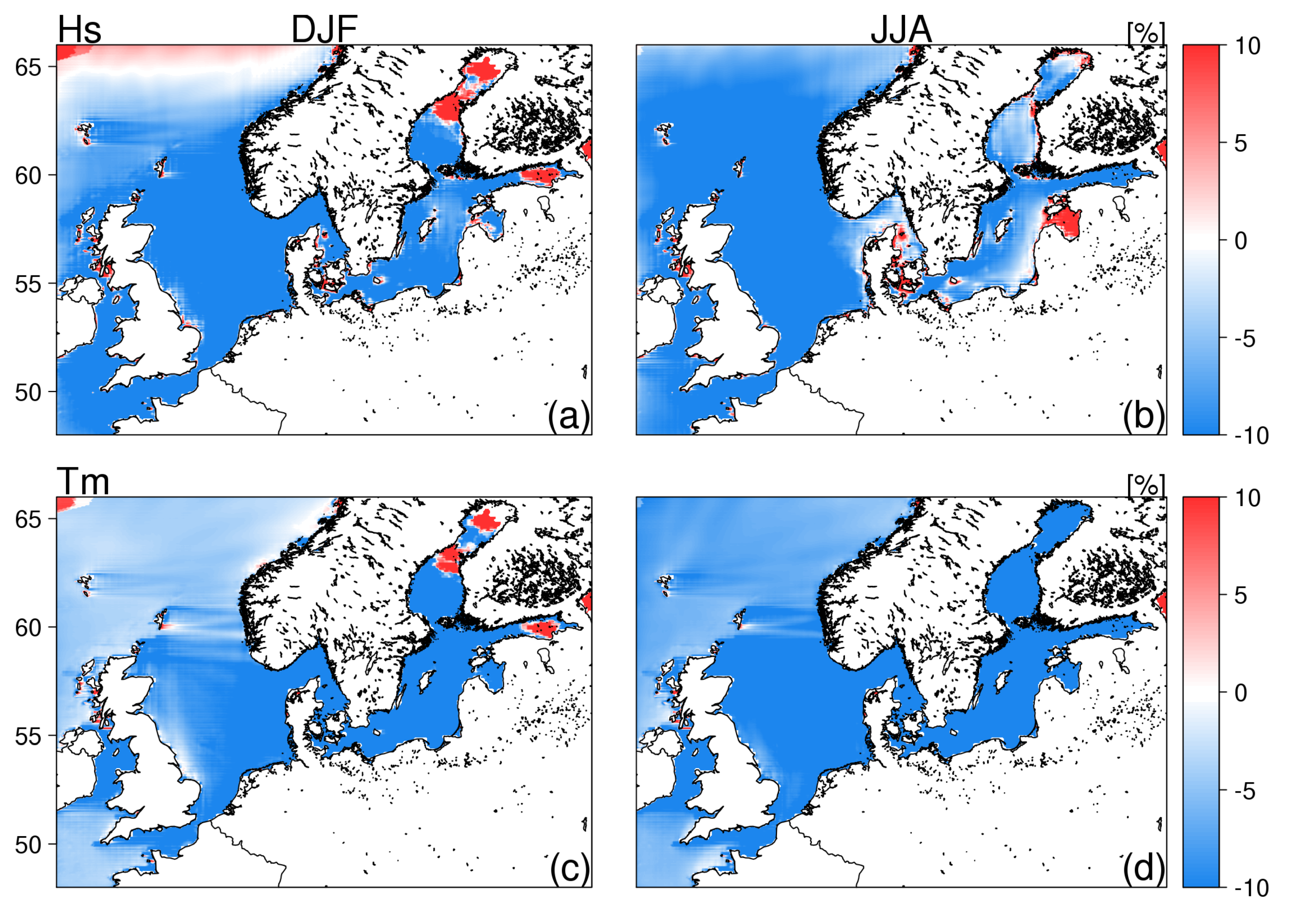
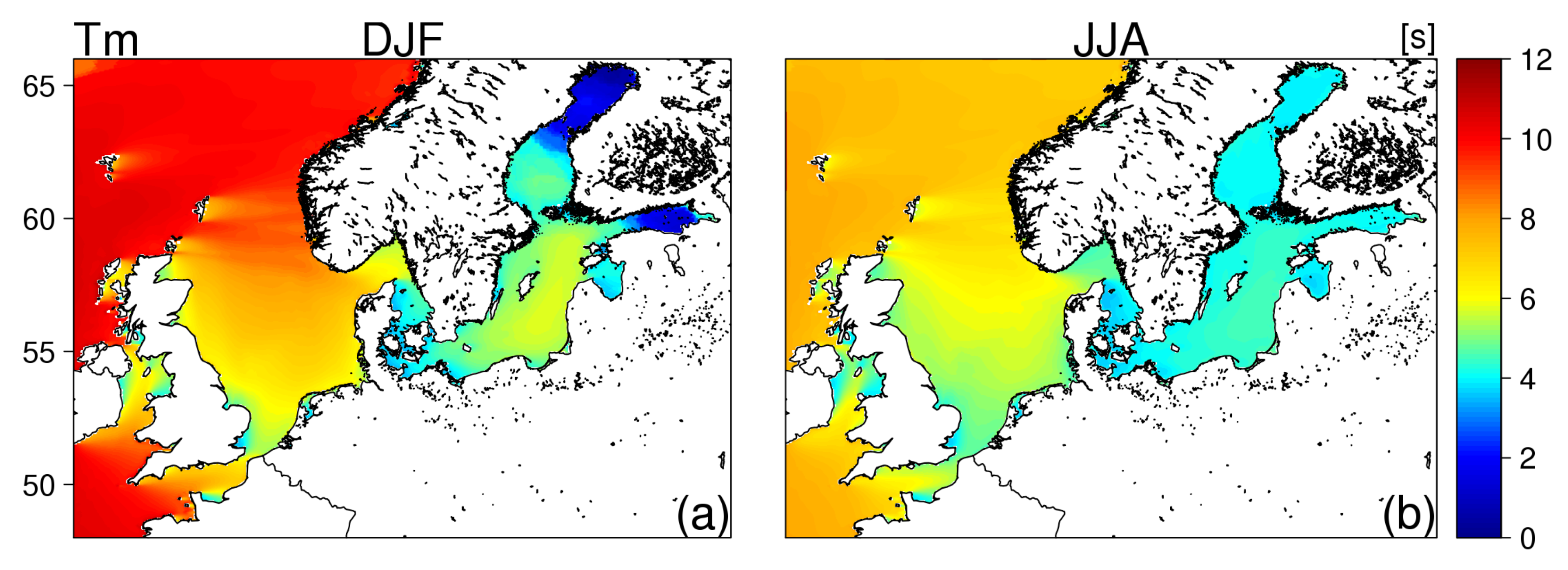
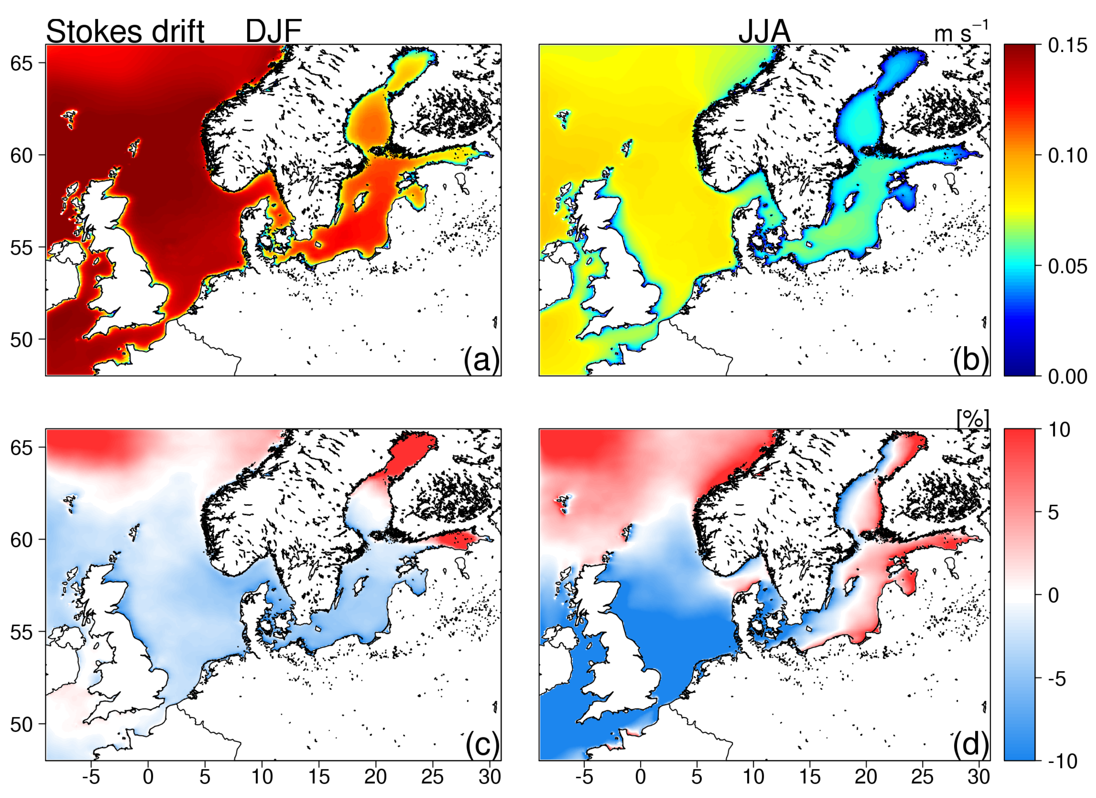
4. Wave Climate Projection (2075–2100)

In this section, we show the results obtained by comparing the historical and future runs to assess the change in the wave climate over the regional domain considered under the RCP8.5 scenario. Figure 10, Figure 11, Figure 12 and Figure 13 show the results obtained in the historical run (top panels) and the differences between the historical and future integrations (bottom panels) over a 25-year period when considering the 95th percentiles of 10 m wind speed, significant wave height, mean wave period and surface Stokes drift speed, respectively. In the following part of this section, the results are presented in terms of relative differences in the future integration, R D f , which is defined as:
R D f = W A M f W A M W A M 100
where W A M and W A M f are the historical and future runs, respectively. Positive (negative) values of R D f mean that the signals in the future projection increased (decreased) in comparison to those in the historical run.
The range of projected wave climate changes (±10%) in the study area reflects those observed by previous global (e.g., [2]) and regional (e.g., [19]) studies. The most interesting feature is the projected increase in the extreme values of all variables in the Northeast Atlantic, except for the mean wave period. Another distinct feature is the projected decrease in extreme values in the North Sea. This is in agreement with the findings of [3], which investigated projected changes in mean significant wave heights under the RCP8.5 scenario and observed similar wave climate change patterns over the same areas. In particular, they underline the role of sea ice extent which has an impact on the fetch available over which to grow waves, and argue that the increase of mean and severe wave conditions in the Northeast Atlantic (north of 60 N) can be partially caused by a reduction in sea ice due to global warming, leading to increased fetch for northerly winds in Nordic Seas.
The projected wind speed (Figure 10) shows an increase in the Northeast Atlantic and North Baltic Sea and a decrease in the North Sea. The annual percentile H s and its projected change (Figure 11) show similarities with changes in the wind field. A general decrease is found in the North Sea, which is in line with the findings of [19,20] over the same area. Similar patterns are observed in the SK subregion and southern part of the Baltic Sea, while an increase is observed in the Gulf of Bothnia, which is in agreement with the findings of [21].
The increase in significant wave heights (Figure 11) in the Northeast Atlantic is not depicted in the results obtained by [19], which instead observed a decrease over the same area and an increase over the Norwegian Sea and the Barents Sea; these results show the differences between the ensemble approach used by the authors to force coarse-resolution (50 km) wave integrations and the single-forced, high-resolution regional wave modelling approach used in this study.
An interesting feature was observed in this area during summer, where a decrease along the Swedish coast and an increase along the Finnish coasts and Gulf of Finland were observed (Figure 11, panel d), which was probably due to changes in dominant meridional winds. The changes in the wind field partially reflect this pattern (Figure 10) and, as expected, are smaller than those in H s due to the quadratic relation between the fully developed wind sea and the wind speed [55]. Considering the mean wave period, the smallest differences between the historical and future changes were observed. Figure 12 shows the 95th percentile of the mean wave period and its projected changes. RD f values smaller than 5% were observed during winter and summer. Larger positive RD f values were found in the Baltic Sea during winter and in the Irish Sea during summer. The impact on surface Stokes drift (Figure 13) was very similar to the changes found in the wind speed and H s . A positive RD f up to the 10% was observed in the Northeast Atlantic in DJF and JJA and in the Baltic Sea during winter. A general decrease (RD f < 10 % ) was observed in the North Sea during summer. During this season, the changes observed considering H s in the Baltic Sea were also reflected by the changes in Stokes drift, even though it was a smaller magnitude.
To investigate the changes in spatial leading modes in wave climate projections, the EOF analysis was also performed by considering H s in the future run (Figure 9). The percentage variance represented by the first leading modes in the future run (e.g., Table 3) was comparable with that observed in the historical run, but looking at their patterns shows that both similarities and distinguishing features can be noticed. The EOF1 shows its maximum variance in the northern part of the North Sea during DJF, which has a pattern similar to that observed in the historical run (Figure 7). In agreement with the results observed considering R D f , the largest differences between the historical and future run were observed during JJA. In this season, EOF1 in the future run showed a significant increase in variance with respect to the historical run in the Northeast Atlantic and a decrease in the southern parts of the North and Baltic Seas. Different patterns can also be noticed during the same season in the Gulf of Bothnia, which is associated with increased variance in the leading mode of the future run. EOF2 in the future run (Figure 9, bottom panels) shows a higher variance in the Northeast Atlantic and Baltic Sea during DJF. An EOF analysis was also performed by considering Stokes drift in the future run (not shown). The main differences with the historical run follow the patterns observed in the H s EOFs, showing an increase in the variance in the signal in the North Atlantic and the northern part of the Baltic Sea during JJA and a decrease in the North Sea and southern part of the Baltic Sea during the same season.
Projected mean wave climate change follows similar geographical patterns compared with the 95th percentile difference patterns (Figure A3, Figure A4, Figure A5 and Figure A6). The main differences can be noticed in the Baltic Sea, where 10% increases in wind speed, significant wave height and mean wave period during summer were observed during summer, which is in line with the findings of other authors in the literature (e.g., [56]), who describe homogeneous increased significant wave heights in this area.

5. Summary and Conclusions

The wave climates in the North Sea, Northeast Atlantic and Baltic Sea were assessed by means of a wave climate simulation under a high emission scenario (RCP8.5). The experiment was designed to span historical (1980–2005) and future (2075–2100) periods to investigate the projected regional wave climate change by the end of the 21st century with respect to the present climate. The wave climate during the historical period (1980–2005) was compared against in situ (GTS and CMEMS data) and remote sensing (i.e., Jason-1) observations, as well as ERA5 and NORA10 hindcasts. Compared with in situ data, at the observation positions, the results showed that the skill of ERA5-h was almost ideal when considering both the whole domain (Figure 2) and subregional domains (Figure 3), which was probably due to the impact of the observed atmospheric data assimilated by the system to obtain an accurate wave hindcast. NORA10-h was also well correlated with the in situ observations but with errors (i.e., NRMSE) that ranged from 10% to 20% of the mean observed signals. Larger errors (20% to 30% ) were observed when considering the historical run. In particular, the results showed that the climate simulation performed better in the areas characterized by large significant wave heights (e.g., North Atlantic and North Sea) than in enclosed basins (e.g., the SK and BA subdomains; Figure 3, bottom panels). These results were confirmed by comparing them with the H s remote sensing data of Jason-1, which overlapped the historical run from 2002 to 2005 (Figure 5). A PC analysis showed that the temporal leading modes obtained from in situ data were well correlated with those of the historical run considering the annual cycle and intra-annual variability at the regional scale (Figure 4). Considering different spatial subdomains (Figure 1), these results were confirmed by only looking at PC2 in the North Atlantic and North Sea, while this was not the case considering the Danish Straits (i.e., SK domain) and Baltic Sea during winter, which was probably due to the coarser spatial and spectral resolutions of the wave model used in this study, which do not allow us to correctly resolve the wave dynamics in these areas. Interestingly, the same was also observed when considering NORA10-h, which failed to capture PC2 in these areas, and a lower accuracy was also observed by considering ERA5-h during winter. At the regional scale, the historical run was compared with ERA5-h (1980–2005) and NORA10-h (1980–2001) in terms of relative difference ( R D h ). The differences observed considering the annual 95th percentiles (Figure 6) follow similar spatial distributions as those observed considering the mean differences (Figure A2). In general, the historical run tended to overestimate by more than 10% of the annual 95th percentile wind speeds and significant wave heights in ERA5-h regardless of the spatial domain and considered season when considering both wind speed and significant wave height; however, more variable patterns were observed when compared with NORA10-h during DJF in the North Atlantic, the eastern part of the North Sea and the Baltic Sea. Positive R D h values were also observed during JJA over the SK domain (Figure 6, bottom right panel). Looking at the spatial leading modes (i.e., EOFs) of significant wave heights, the results showed coherent patterns between the historical run and ERA5-h (Figure 7 and Figure 8) during winter, while discrepancies were observed in summer in the Baltic Sea considering EOF1 and in the northern part of the North Sea (Norwegian Trench) considering EOF2 during the same season.
Looking at future wave climate projections, similar R D f patterns were observed when considering both mean (Figure A3, Figure A4, Figure A5 and Figure A6) and severe (Figure 10, Figure 11, Figure 12 and Figure 13) wave conditions, which were generally larger during JJA. The most interesting feature is the projected increases in extreme wind speed, surface Stokes drift and significant wave height in the Northeast Atlantic, which had similar ranges (10%) compared to those observed by [2] over the same area. An increase in wave conditions in this area was also observed by [3], which argued that increased wave heights to the North of Scotland may be related to Arctic sea-ice retreat, due to global warming and leading to increased fetch for northerly winds in Nordic Seas. In this area (NA sub-domain, Figure 1), Ref. [19] instead observed relative differences in significant wave heights that were close to zero, which was probably due to the multimodel ensemble approach used by the authors and the different historical period (i.e., 1971–2000) considered to quantify the projected wave climate changes. On the other hand, a decrease larger than 10% was observed in the North Sea, confirming the results of [20] in the western part of the basin. The authors observed also an increase in the mean and extreme values in the eastern part of the North Sea, which was not noticed in this study, indicating discrepancies due to different experimental designs used (in terms of forcings (single and multimodel), scenarios (CMIP5 and SRES) and wave model (e.g., 5 km and 50 km spatial resolutions)). Interesting features were observed in the Baltic regarding the change in annual percentiles (10 m wind speed, H s , and surface Stokes drift). A decrease was observed in the southern part of the subdomain, which was associated with increased extreme values in the Gulf of Bothnia during winter. This is in agreement with [21], who observed incoherent variation patterns when looking at the projected changes in extreme wave height in the basin. During summer, a decrease along the Swedish coast and an increase along the Finnish coasts and Gulf of Finland were observed, which was probably due to changes in dominant meridional winds. The spatial leading modes extracted from the future run showed patterns of variability that were similar to those of the historical run during DJF and JJA and those of ERA5-h in the Baltic Sea (EOF2 JJA) and the northern part of the North Sea (EOF2 DJF).
In general, the range of variation in the projected extremes (±10%) was consistent with those observed by other authors both at the global (e.g., [2]) and regional (e.g., [20]) spatial scales. Nonetheless, it is very important to notice that this range of change is on the order of the relative difference between the historical run and the wave hindcasts and that the error with respect to the observations is even larger. These findings bring uncertainty to the possible conclusions that can be drawn when investigating wave climate projections at the regional scale.
Ensemble methods are typically used to reduce the uncertainty and increase the accuracy of global wave climate simulation (e.g., [1]). In the future, a multimodel ensemble approach should also be used in regional wave climate studies, including dynamical downscaling of the forcings to be used in the regional wave climate simulations. In this context, high-resolution wave models accounting for the ocean wave-current interactions [57] should also be used, especially over regional scales, to obtain a realistic representation of the physical processes in the ocean that characterize the reciprocated interactions in Earth’s climate system.

Author Contributions

A.B. (Antonio Bonaduce) processed and interpreted the data and wrote the paper; J.S. participated in the experimental design and wave model set-up, interpreted the data and significantly contributed to elaborate the structure of the manuscript; A.B. (Arno Behrens) participated in the experimental design, was responsible for the model set-up, performed the wave climate simulation and contributed to the manuscript; J.-R.B. participated in the experimental design, provided ERA5-hindcast and GTS in situ data, and contributed to the manuscript; R.A.I.W. provided the RA4 forcing data and contributed to the manuscript.

Funding

Antonio Bonaduce was supported by the Initiative and Networking Fund of the Helmholtz Association through the project “Advanced Earth System Modelling Capacity (ESM)”.

Acknowledgments

The numerical simulation was performed using the high-performance computer at the German Climate Computing Center (DKRZ). Alvaro Semedo (IHE-Delft) significantly contributed to the experimental design and provided useful comments about the manuscript. Gil Lemos (University of Lisbon) provided the NORA10-hindcast data. Jean-Raymond Bidlot and Joanna Staneva gratefully acknowledge support from the Copernicus Marine Environmental Monitoring Service (CMEMS) and Mercator Ocean through the WaveFlow Service Evolution project.

Conflicts of Interest

The authors declare no conflict of interest.

Appendix A. Mean Wave Climate Change

Figure A1. Average significant wave height, H s (panels a and b), mean wave period (panels c and d), and 10 m wind speed (panels e and f) from ERA5-h (1980–2005) during winter (DJF; left panels) and summer (JJA; right panels).
Jmse 07 00166 g0a1aJmse 07 00166 g0a1b
Figure A2. Average significant wave height, H s (panels a and b), mean wave period (panels c and d), and 10 m wind speed (panels e and f) normalized difference between ERA5-h (1980–2005) and the historical run during winter (DJF; left panels) and summer (JJA; right panels).
Jmse 07 00166 g0a2aJmse 07 00166 g0a2b
Figure A3. Average 10 m wind speed (panels a and b) from the historical run and the normalized difference (panels c and d) between the future run and historical run during winter (DJF; left panels) and summer (JJA; right panels).
Jmse 07 00166 g0a3
Figure A4. Average significant wave height, H s (panels a and b) from the historical run and the normalized difference (panels c and d) between the future run and historical run during winter (DJF; left panels) and summer (JJA; right panels).
Jmse 07 00166 g0a4
Figure A5. Average mean wave period, T m (panels a and b), from the historical run and the normalized difference (panels c and d) between the future run and historical run during winter (DJF; left panels) and summer (JJA; right panels).
Jmse 07 00166 g0a5aJmse 07 00166 g0a5b
Figure A6. Average surface Stokes drift speed (panels a and b) from the historical run and the normalized difference (panels c and d) between the future run and historical run during winter (DJF; left panels) and summer (JJA; right panels).
Jmse 07 00166 g0a6

References

  1. Hemer, M.A.; Fan, Y.; Mori, N.; Semedo, A.; Wang, X.L. Projected changes in wave climate from a multi-model ensemble. Nat. Clim. Chang. 2013, 3, 471. [Google Scholar] [CrossRef]
  2. Breivik, Ø.; Carrasco, A.; Staneva, J.; Behrens, A.; Semedo, A.; Bidlot, J.R.; Aarnes, O.J. Global Stokes Drift Climate under the RCP8.5 Scenario. J. Clim. 2019, 32, 1677–1691. [Google Scholar] [CrossRef]
  3. Bricheno, L.M.; Wolf, J. Future Wave Conditions of Europe, in Response to High-End Climate Change Scenarios. J. Geophys. Res. Ocean. 2018, 123, 8762–8791. [Google Scholar] [CrossRef]
  4. Wolf, J.; Woolf, D.K. Waves and climate change in the north-east Atlantic. Geophys. Res. Lett. 2006, 33. [Google Scholar] [CrossRef] [Green Version]
  5. Semedo, A.; Dobrynin, M.; Lemos, G.; Behrens, A.; Staneva, J.; de Vries, H.; Sterl, A.; Bidlot, J.R.; Miranda, P.M.A.; Murawski, J. CMIP5-Derived Single-Forcing, Single-Model, and Single-Scenario Wind-Wave Climate Ensemble: Configuration and Performance Evaluation. J. Mar. Sci. Eng. 2018, 6, 90. [Google Scholar] [CrossRef]
  6. Stocker, T.; Qin, D.; Plattner, G.K.; Alexander, L.; Allen, S.; Bindoff, N.; Breon, F.M.; Church, J.; Cubasch, U.; Emori, S.; et al. Technical Summary. In Climate Change 2013: The Physical Science Basis. Contribution of Working Group I to the Fifth Assessment Report of the Intergovernmental Panel on Climate Change; Stocker, T., Qin, D., Plattner, G.K., Tignor, M., Allen, S., Boschung, J., Nauels, A., Xia, Y., Bex, V., Midgley, P., Eds.; Cambridge University Press: Cambridge, UK; New York, NY, USA, 2013; pp. 33–115. [Google Scholar] [CrossRef]
  7. Rhein, M.; Rintoul, S.; Aoki, S.; Campos, E.; Chambers, D.; Feely, R.; Gulev, S.; Johnson, G.; Josey, S.; Kostianoy, A.; et al. Observations: Ocean. In Climate Change 2013: The Physical Science Basis. Contribution of Working Group I to the Fifth Assessment Report of the Intergovernmental Panel on Climate Change; Stocker, T., Qin, D., Plattner, G.K., Tignor, M., Allen, S., Boschung, J., Nauels, A., Xia, Y., Bex, V., Midgley, P., Eds.; Cambridge University Press: Cambridge, UK; New York, NY, USA, 2013; pp. 255–316. [Google Scholar] [CrossRef]
  8. Church, J.; Clark, P.; Cazenave, A.; Gregory, J.; Jevrejeva, S.; Levermann, A.; Merrifield, M.; Milne, G.; Nerem, R.; Nunn, P.; et al. Sea Level Change. In Climate Change 2013: The Physical Science Basis. Contribution of Working Group I to the Fifth Assessment Report of the Intergovernmental Panel on Climate Change; Stocker, T., Qin, D., Plattner, G.K., Tignor, M., Allen, S., Boschung, J., Nauels, A., Xia, Y., Bex, V., Midgley, P., Eds.; Cambridge University Press: Cambridge, UK; New York, NY, USA, 2013; pp. 1137–1216. [Google Scholar] [CrossRef]
  9. Cavaleri, L.; Fox-Kemper, B.; Hemer, M. Wind Waves in the Coupled Climate System. Bull. Am. Meteorol. Soc. 2012, 93, 1651–1661. [Google Scholar] [CrossRef]
  10. Lemos, G.; Semedo, A.; Dobrynin, M.; Behrens, A.; Staneva, J.; Bidlot, J.R.; Miranda, P.M. Mid-twenty-first century global wave climate projections: Results from a dynamic CMIP5 based ensemble. Glob. Planet. Chang. 2019, 172, 69–87. [Google Scholar] [CrossRef]
  11. Taylor, K.E.; Stouffer, R.J.; Meehl, G.A. An Overview of CMIP5 and the Experiment Design. Bull. Am. Meteorol. Soc. 2012, 93, 485–498. [Google Scholar] [CrossRef] [Green Version]
  12. Moss, R.H.; Edmonds, J.A.; Hibbard, K.A.; Manning, M.R.; Rose, S.K.; Van Vuuren, D.P.; Carter, T.R.; Emori, S.; Kainuma, M.; Kram, T.; et al. The next generation of scenarios for climate change research and assessment. Nature 2010, 463, 747. [Google Scholar] [CrossRef]
  13. Nakicenovic, N.; Alcamo, J.; Grubler, A.; Riahi, K.; Roehrl, R.; Rogner, H.H.; Victor, N. Special Report on Emissions Scenarios (SRES), A Special Report of Working Group III of the Intergovernmental Panel on Climate Change; Cambridge University Press: Cambridge, UK, 2000. [Google Scholar]
  14. Bitner-Gregersen, E.M.; Vanem, E.; Gramstad, O.; Hørte, T.; Aarnes, O.J.; Reistad, M.; Breivik, Ø.; Magnusson, A.K.; Natvig, B. Climate change and safe design of ship structures. Ocean Eng. 2018, 149, 226–237. [Google Scholar] [CrossRef] [Green Version]
  15. Dobrynin, M.; Murawski, J.; Baehr, J.; Ilyina, T. Detection and Attribution of Climate Change Signal in Ocean Wind Waves. J. Clim. 2015, 28, 1578–1591. [Google Scholar] [CrossRef] [Green Version]
  16. Wang, X.L.; Feng, Y.; Swail, V.R. Changes in global ocean wave heights as projected using multimodel CMIP5 simulations. Geophys. Res. Lett. 2014, 41, 1026–1034. [Google Scholar] [CrossRef]
  17. Casas-Prat, M.; Wang, X.; Swart, N. CMIP5-based global wave climate projections including the entire Arctic Ocean. Ocean Model. 2018, 123, 66–85. [Google Scholar] [CrossRef]
  18. Erikson, L.; Hegermiller, C.; Barnard, P.; Ruggiero, P.; van Ormondt, M. Projected wave conditions in the Eastern North Pacific under the influence of two CMIP5 climate scenarios. Ocean Model. 2015, 96, 171–185. [Google Scholar] [CrossRef]
  19. Aarnes, O.J.; Reistad, M.; Breivik, Ø.; Bitner-Gregersen, E.; Ingolf Eide, L.; Gramstad, O.; Magnusson, A.K.; Natvig, B.; Vanem, E. Projected changes in significant wave height toward the end of the 21st century: Northeast Atlantic. J. Geophys. Res. Ocean. 2017, 122, 3394–3403. [Google Scholar] [CrossRef] [Green Version]
  20. Grabemann, I.; Groll, N.; Möller, J.; Weisse, R. Climate change impact on North Sea wave conditions: A consistent analysis of ten projections. Ocean Dyn. 2015, 65, 255–267. [Google Scholar] [CrossRef]
  21. Groll, N.; Grabemann, I.; Hünicke, B.; Meese, M. Baltic Sea wave conditions under climate change scenarios. Boreal Environ. Res. 2017, 22, 1–12. [Google Scholar]
  22. Cavaleri, L.; Abdalla, S.; Benetazzo, A.; Bertotti, L.; Bidlot, J.R.; Breivik, Ø.; Carniel, S.; Jensen, R.; Portilla-Yandun, J.; Rogers, W.; et al. Wave modelling in coastal and inner seas. Prog. Oceanogr. 2018, 167, 164–233. [Google Scholar] [CrossRef]
  23. WAMDI-Group. The WAM Model - A Third Generation Ocean Wave Prediction Model. J. Phys. Oceanogr. 1988, 18, 1775–1810. [Google Scholar] [CrossRef]
  24. Komen, G.J.; Hasselmann, K.; Cavaleri, L.; Donelan, M.; Janssen, P.A.E.M.; Hasselmann, S. Dynamics and Modelling of Ocean Waves. J. Fluid Mech. 1994, 307, 375–376. [Google Scholar] [CrossRef]
  25. Günther, H.; Hasselmann, S.; Janssen, P. The WAM Model Cycle 4.0. User Manual; Technical Report; Deutsches Klimarechenzentrum: Hamburg, Germany, 1992. [Google Scholar]
  26. ECMWF. Part VII: ECMWF Wave Model. In IFS Documentation CY45R1; Number 7 in IFS Documentation CY45R1; ECMWF: Reading, UK, 2018. [Google Scholar]
  27. Staneva, J.; Behrens, A.; Wahle, K. Wave modelling for the German Bight coastal-ocean predicting system. J. Phys. Conf. Ser. 2015, 633, 012117. [Google Scholar] [CrossRef]
  28. Strandberg, G.; Bärring, L.; Hansson, U.; Jansson, C.; Jones, C.; Kjellström, E.; Kupiainen, M.; Nikulin, G.; Samuelsson, P.; Ullerstig, A. CORDEX Scenarios for Europe from the Rossby Centre Regional Climate Model RCA4; Technical Report 116; Climate research–Rossby Centre: Norrkoping, Sweden, 2015. [Google Scholar]
  29. Hazeleger, W.; Severijns, C.; Semmler, T.; Ştefănescu, S.; Yang, S.; Wang, X.; Wyser, K.; Dutra, E.; Baldasano, J.M.; Bintanja, R.; et al. EC-Earth. Bull. Am. Meteorol. Soc. 2010, 91, 1357–1364. [Google Scholar] [CrossRef] [Green Version]
  30. Hazeleger, W.; Wang, X.; Severijns, C.; Ştefănescu, S.; Bintanja, R.; Sterl, A.; Wyser, K.; Semmler, T.; Yang, S.; van den Hurk, B.; et al. EC-Earth V2.2: Description and validation of a new seamless earth system prediction model. Clim. Dyn. 2012, 39, 2611–2629. [Google Scholar] [CrossRef]
  31. Brodeau, L.; Koenigk, T. Extinction of the northern oceanic deep convection in an ensemble of climate model simulations of the 20th and 21st centuries. Clim. Dyn. 2016, 46, 2863–2882. [Google Scholar] [CrossRef]
  32. Caian, M.; Koenigk, T.; Döscher, R.; Devasthale, A. An interannual link between Arctic sea-ice cover and the North Atlantic Oscillation. Clim. Dyn. 2018, 50, 423–441. [Google Scholar] [CrossRef]
  33. Hersbach, H.; Dee, D. ERA5 reanalysis is in production. ECMWF Newslett. 2016, 147, 7. [Google Scholar]
  34. Reistad, M.; Breivik, Ø.; Haakenstad, H.; Aarnes, O.J.; Furevik, B.R.; Bidlot, J.R. A high-resolution hindcast of wind and waves for the North Sea, the Norwegian Sea, and the Barents Sea. J. Geophys. Res. Ocean. 2011, 116. [Google Scholar] [CrossRef] [Green Version]
  35. Bidlot, J.R.; Holt, M.W. Verification of Operational Global and Regional Wave Forecasting Systems against Measurements from Moored Buoys; Jcomm Technical Report; WMO & IOC: Geneva, Switzerland, 2006. [Google Scholar]
  36. Bidlot, J.R.; Holmes, D.J.; Wittmann, P.A.; Lalbeharry, R.; Chen, H.S. Intercomparison of the Performance of Operational Ocean Wave Forecasting Systems with Buoy Data. Weather Forecast. 2002, 17, 287–310. [Google Scholar] [CrossRef]
  37. Passaro, M.; Cipollini, P.; Vignudelli, S.; Quartly, G.D.; Snaith, H.M. ALES: A multi-mission adaptive subwaveform retracker for coastal and open ocean altimetry. Remote Sens. Environ. 2014, 145, 173–189. [Google Scholar] [CrossRef] [Green Version]
  38. Passaro, M.; Fenoglio-Marc, L.; Cipollini, P. Validation of Significant Wave Height From Improved Satellite Altimetry in the German Bight. IEEE Trans. Geosci. Remote Sens. 2015, 53, 2146–2156. [Google Scholar] [CrossRef]
  39. Uppala, S.M.; Kållberg, P.; Simmons, A.; Andrae, U.; Bechtold, V.D.C.; Fiorino, M.; Gibson, J.; Haseler, J.; Hernandez, A.; Kelly, G.; et al. The ERA-40 re-analysis. Q. J. R. Meteorol. Soc. 2005, 131, 2961–3012. [Google Scholar] [CrossRef]
  40. Aarnes, O.J.; Breivik, Ø.; Reistad, M. Wave Extremes in the Northeast Atlantic. J. Clim. 2012, 25, 1529–1543. [Google Scholar] [CrossRef] [Green Version]
  41. Semedo, A.; Vettor, R.; Breivik, Ø.; Sterl, A.; Reistad, M.; Soares, C.G.; Lima, D. The wind sea and swell waves climate in the Nordic seas. Ocean Dyn. 2015, 65, 223–240. [Google Scholar] [CrossRef]
  42. Undén, P.; Rontu, L.; Jarvinen, H.; Lynch, P.; Calvo Sánchez, F.J.; Cats, G.; Cuxart, J.; Eerola, K.; Fortelius, C.; Garcia-Moya, J.A.; et al. HIRLAM-5 Scientific Documentation; Swedish Meteorological and Hydrological Institute: Norrkoping, Sweden, 2002. [Google Scholar]
  43. Bruserud, K.; Haver, S. Comparison of wave and current measurements to NORA10 and NoNoCur hindcast data in the northern North Sea. Ocean Dyn. 2016, 66, 823–838. [Google Scholar] [CrossRef]
  44. Dee, D.P.; Uppala, S.M.; Simmons, A.; Berrisford, P.; Poli, P.; Kobayashi, S.; Andrae, U.; Balmaseda, M.; Balsamo, G.; Bauer, d.P.; et al. The ERA-Interim reanalysis: Configuration and performance of the data assimilation system. Q. J. R. Meteorol. Soc. 2011, 137, 553–597. [Google Scholar] [CrossRef]
  45. ECMWF. ERA5 Documentation. Available online: https://confluence.ecmwf.int/label/CKB/era5 (accessed on 14 March 2019).
  46. Wiese, A.; Staneva, J.; Schulz-Stellenfleth, J.; Behrens, A.; Fenoglio-Marc, L.; Bidlot, J.R. Synergy of wind wave model simulations and satellite observations during extreme events. Ocean Sci. 2018, 14, 1503–1521. [Google Scholar] [CrossRef] [Green Version]
  47. Hersbach, H.; de Rosnay, P.; Bell, B.; Schepers, D.; Simmons, A.; Soci, C.; Abdalla, S.; Alonso-Balmaseda, M.; Balsamo, G.; Bechtold, P.; et al. Operational Global Reanalysis: Progress, Future Directions and Synergies with NWP; European Centre for Medium Range Weather Forecasts: Reading, UK, 2018. [Google Scholar]
  48. ECMWF. ECMWF Wave Model. In IFS Documentation CY46R1; IFS Documentation CY46R1; ECMWF: Reading, UK, 2019. [Google Scholar]
  49. Bidlot, J.R.; Janssen, P.A.E.M.; Abdalla, S. A revised formulation of ocean wave dissipation and its model impact. In ECMWF Technical Memorandum; ECMWF: Reading, UK, 2007; p. 27. [Google Scholar] [CrossRef]
  50. Ardhuin, F.; Rogers, E.; Babanin, A.V.; Filipot, J.F.; Magne, R.; Roland, A.; van der Westhuysen, A.; Queffeulou, P.; Lefevre, J.M.; Aouf, L.; et al. Semiempirical Dissipation Source Functions for Ocean Waves. Part I: Definition, Calibration, and Validation. J. Phys. Oceanogr. 2010, 40, 1917–1941. [Google Scholar] [CrossRef] [Green Version]
  51. Bidlot, J.R. Ocean Wave Model Output Parameters. 2016. Available online: https://software.ecmwf.int/wiki/display/IFS/Official+IFS+Documentation (accessed on 15 January 2019).
  52. Semedo, A.; Weisse, R.; Behrens, A.; Sterl, A.; Bengtsson, L.; Günther, H. Projection of Global Wave Climate Change toward the End of the Twenty-First Century. J. Clim. 2013, 26, 8269–8288. [Google Scholar] [CrossRef]
  53. von Storch, H. Spatial Patterns: EOFs and CCA. In Analysis of Climate Variability: Applications of Statistical Techniques; von Storch, H., Navarra, A., Eds.; Springer: Berlin/Heidelberg, Germany, 1995; pp. 227–257. [Google Scholar] [CrossRef]
  54. Björnsson, H.; Venegas, S. A manual for EOF and SVD analyses of climatic data. CCGCR Rep. 1997, 97, 112–134. [Google Scholar]
  55. Pierson, W.J., Jr.; Moskowitz, L. A proposed spectral form for fully developed wind seas based on the similarity theory of S. A. Kitaigorodskii. J. Geophys. Res. 1964, 69, 5181–5190. [Google Scholar] [CrossRef]
  56. Morim, J.; Hemer, M.; Cartwright, N.; Strauss, D.; Andutta, F. On the concordance of 21st century wind-wave climate projections. Glob. Planet. Chang. 2018, 167, 160–171. [Google Scholar] [CrossRef]
  57. Staneva, J.; Alari, V.; Breivik, Ø.; Bidlot, J.R.; Mogensen, K. Effects of wave-induced forcing on a circulation model of the North Sea. Ocean Dyn. 2017, 67, 81–101. [Google Scholar] [CrossRef]
Figure 1. Observational network used to assess the reliability of wave climate simulation over the historical period (1980–2005). In situ observation positions and satellite tracks of the Jason-1 mission are shown as red dots and black lines, respectively. Frames show the subregions considered: Northeast Atlantic (NA), North Sea (NS), Skagerrak and Kattegat (SK) and the Baltic Sea (BA). Background: bathymetry of the WAM (m).
Jmse 07 00166 g001
Figure 2. Julian year daily means of the significant wave height, H s (m), at the observation positions during the historical run period (1980–2005) for in situ observations (blue line), ERA5-hindcast (green line) and wave model (red line, WAM) over the whole model domain (Figure 1).
Jmse 07 00166 g002
Figure 3. As in Figure 2 but considering data at observation positions in the (a) Northeast Atlantic; (b) North Sea; (c) Baltic Sea and (d) Skagerrak-Kattegat areas.
Jmse 07 00166 g003
Figure 4. As in Figure 3 but considering PCs. In the panels: first (a) and second (b) PCs considering data at observation positions over the whole domain; the other panels show the second PC considering data at observation positions in the (c) Northeast Atlantic, (d) North Sea, (e) Baltic Sea and (f) Skagerrak-Kattegat areas.
Jmse 07 00166 g004
Figure 5. Comparison with satellite altimetry along-track data: Jason-1 (2001–2005). In the panels: (a) correlation coefficients and (b) NMRSE between significant wave heights from remote sensing and historical run data.
Jmse 07 00166 g005
Figure 6. Annual 95th percentile normalized difference, expressed as a percentage, among ERA5 (1980–2005), NORA10 (1980–2001) and the historical run during winter (DJF; left panels) and summer (JJA; right panels). The panels show the normalized differences between the historical run (10 m wind speed) and ERA5 (panels a and b) significant wave height, H s , and the ERA5-hindcast (panels c and d) significant wave height, H s , and NORA10-hindcast (panels e and f).
Jmse 07 00166 g006
Figure 7. Significant wave height, H s , EOF1 considering ERA5-hindcast (1980–2005; panels a and b) and the historical run (1980–2005; panels c and d) during winter (DJF; left panels) and summer (JJA; right panels).
Jmse 07 00166 g007
Figure 8. As in Figure 7 but considering EOF2.
Jmse 07 00166 g008
Figure 9. Significant wave height, H s , first (panels a and b) and second (panels c and d) EOFs considering the future run (2075–2100) during winter (DJF; left panels) and summer (JJA; right panels).
Jmse 07 00166 g009
Figure 10. Annual 95th percentile 10 m wind speed (panels a and b) from the historical run and the normalized difference (panels c and d) between the future run and historical run during winter (DJF; left panels) and summer (JJA; right panels).
Jmse 07 00166 g010
Figure 11. Annual 95th percentile significant wave height, H s , (panels a and b) from the historical run and the normalized difference (panels c and d) between the future run and historical run during winter (DJF; left panels) and summer (JJA; right panels).
Jmse 07 00166 g011aJmse 07 00166 g011b
Figure 12. As in Figure 11 but considering the mean wave period, T m .
Jmse 07 00166 g012
Figure 13. As in Figure 11 but considering surface Stokes drift speed.
Jmse 07 00166 g013
Table 1. Significant wave height, H s , comparison between the wave model (WAM), ERA5-hindcast (ERA5-h) and NORA10-hindcast (NORA10-h) with in situ observations during the historical period (1980–2005). The column values show basic statistics of the compared datasets: correlation coefficient (C), BIAS, and NRMSE.
ERA5-h NORA10-h WAM
C BIAS NRMSE C BIAS NRMSE C BIAS NMRSE
FULL0.990.097.780.930.0612.280.890.1820.22
NA0.99−0.012.960.91−0.0515.080.880.1318.75
NS0.990.023.690.920.0916.240.760.1724.98
SK0.960.0412.560.800.0123.630.640.0734.77
BA0.980.048.160.950.0915.980.710.1531.3
Table 2. Significant wave height, H s , and PCs. Columns 1–3: percent variance explained by the three leading PCs obtained considering ERA5-hindcast (ERA5-h), NORA10-hindcast (NORA10-h) and the historical run (WAM) at the observation (OBS) positions during the period (1980–2005), respectively. Columns 4–6: correlation coefficients between the observed H s PCs and those obtained from the ERA5-hindcast (C E R A 5 h ), NORA10 hindcast (C N O R A 10 h ) and the historical run (C W A M h ), respectively.
OBSERA5-hNORA10-hWAMC ERA 5 h C NORA 10 h C WAM
PC1(FULL)46.5348.2440.7947.990.990.940.91
PC2(FULL)10.8411.4410.398.190.980.660.51
PC1(NA)60.5463.0357.3265.600.990.910.89
PC2(NA)13.7713.0512.7810.030.990.570.6
PC1(NS)44.7845.1851.4944.720.990.940.76
PC2(NS)17.2019.5415.8215.840.990.580.36
PC1(SK)34.6532.9947.4840.220.780.250.36
PC2(SK)28.7027.7730.4823.110.680.050.14
PC1(BA)43.8940.6635.3732.930.980.940.74
PC2(BA)11.4312.4112.3213.440.890.360.1
Table 3. Significant wave height, H s , and leading EOFs. The column values show the percent variance explained by the three leading EOFs obtained considering the ERA5-hindcast (ERA5-h) and WAM over historical (WAM; 1980–2005) and future (WAM-f; 2075–2100) periods during winter (DJF; Columns 1–3) and summer (JJA; Columns 4–6).
ERA5-h DJFWAM DJFWAM-f DJFERA5-h JJAWAM JJAWAM-f JJA
EOF1(ALL)58.7658.2961.641.2847.6445.08
EOF2(ALL)15.3715.7216.1022.4618.2620.8
EOF1(NA)90.2287.5492.3277.8781.3386.38
EOF2(NA)4.935.143.1110.176.125.18
EOF1(NS)80.0378.4580.2178.7778.6976.80
EOF2(NS)11.869.2511.129.2010.3412.96
EOF1(SK)82.1069.9376.6773.1368.0858.69
EOF2(SK)9.8814.6710.4316.1018.3724.47
EOF1(BA)57.2662.176064.8061.5657.65
EOF2(BA)13.5313.5117.214.9017.7019.7
Table 4. As in Table 3 but considering Stokes drift leading EOFs.
ERA5-h DJFWAM DJFWAM-f DJFERA5-h JJAWAM JJAWAM-f JJA
EOF1(ALL)50.9748.5652.934.7840.3938.1
EOF2(ALL)18.5719.9221.6422.0519.5922.76
EOF1(NA)77.9765.0279.7559.4970.0177.99
EOF2(NA)8.2517.836.2713.349.678.94
EOF1(NS)83.0880.0081.9172.8171.4765.77
EOF2(NS)9.4711.8011.409.3114.8417.92
EOF1(SK)87.9176.2681.8977.3373.0462.43
EOF2(SK)4.789.407.5913.3314.4221.20
EOF1(BA)56.2969.8964.9963.3361.4657.93
EOF2(BA)13.9212.6715.9715.5418.0419.13

