Article

Bridge Scour Identification and Field Application Based on Ambient Vibration Measurements of Superstructures

1
Department of Bridge Engineering, School of Transportation, Southeast University, Nanjing 211189, China
2
Department of Civil and Environmental Engineering, Louisiana State University, Baton Rouge, LA 70803, USA
3
Research Institute of Highway Ministry of Transport, Beijing 100088, China
4
School of Sustainable Engineering and the Built Environment, Arizona State University, Tempe, AZ 85281, USA
*
Author to whom correspondence should be addressed.
J. Mar. Sci. Eng. 2019, 7(5), 121; https://doi.org/10.3390/jmse7050121
Submission received: 16 March 2019 / Revised: 14 April 2019 / Accepted: 18 April 2019 / Published: 26 April 2019
(This article belongs to the Special Issue Coastal Geohazard and Offshore Geotechnics)

Abstract

:
A scour identification method was developed based on the ambient vibration measurements of superstructures. The Hangzhou Bay Bridge, a cable-stayed bridge with high scour potential, was selected to illustrate the application of this method. Firstly, two ambient vibration measurements were conducted in 2013 and 2016 by installing the acceleration sensors on the girders and pylon. By modal analysis, the natural frequencies of the superstructures were calculated with respect to different mode shapes. Then, by tracing the change of dynamic features between two measurements in 2013 and 2016, the discrepancies of the support boundary conditions, i.e., at the foundation of the Hangzhou Bay Bridge, were detected, which, in turn, qualitatively identified the existence of bridge foundation scour. Secondly, an FE model of the bridge considering soil-pile interaction was established to further quantify the scour depth in two steps. (1) The stiffness of the soil springs representing the support boundary of the bridge was initially identified by the model updating method. In this step, the principle for a successful identification is to make the simulation results best fit the measured natural frequencies of those modes insensitive to the scour. (2) Then, using the updated FE model, the scour depth was identified by updating the depth of supporting soils. In this step, the principle of model updating is to make the simulation results best fit the measured natural frequency changes of those modes sensitive to the scour. Finally, a comparison to the underwater terrain map of the Hangzhou Bay Bridge was carried out to verify the accuracy of the predicted scour depth. Based on the study in this paper, it shows that the proposed method for identifying bridge scour based on the ambient vibration measurements of superstructures is effective and convenient. It is feasible to quickly assess scour conditions for a large number of bridges without underwater devices and operations.

1. Introduction

Bridge scour is a significant concern around the world. In the past 40 years, more than 1500 bridges collapsed, and approximately 60% of these failures are related to the scour of foundations in the United States [1,2]. For example, the catastrophic collapse of the Schoharie Creek Bridge in New York in 1987 was caused by the cumulative effects of pier scour [3]. The Los Gatos Creek Bridge over I-5 in the state of California collapsed because of local pier scour during a flood event, and the underlying reason was due to the channel degradation during the 28 years of service [4]. However, the vulnerability of bridges subject to scouring cannot be predicted by routine hydraulic and geotechnical analyses, because more than 100,000 bridges over water in the United States are identified as “unknown foundations” [4,5].
In China, many cable-supported bridges with super-long spans have been recently constructed over rivers and water channels such as the Yangtze River, Yellow River, Qiantang River, etc. These bridges are enormously vulnerable to the hydrological environments such as the annually typhoon-induced floods. Thus, more serious bridge scour, especially at pylons, occurred very often and developed rapidly. Based on the investigation reports, the scour depths of three typical cable-stayed bridges crossing the Yangtze River in China, i.e., the 2nd Nanjing Yangtze River Bridge, Hangzhou Bay Bridge, and Runyang Yangtze River Bridge, were 20 m, 16 m, and 18 m, respectively [6]. Taking the devastating Typhoon Morakot in the summer of 2009 for a detailed example, as many as 3000 mm of rainfall poured in four days and led to the failures or severe damages of more than 110 bridges [7]. Field investigation indicates that the major cause is foundation scour that removes the bed materials surrounding the piers and abutments. Therefore, it is urgent to develop an effective and economical method to identify bridge scour.
An analytical solution or numerical simulation is the common way to predict the bridge scour depth due to its practical conveniences [8,9,10,11,12,13,14]. Along with continuous scour experiments, these formulas for calculation are similar to the real situations [15,16]. However, some assumptions may still be applied in the formulas in order to reduce their complexity since the number of the selected parameters is limited. Therefore, these formulas may not be able to reflect the real scouring situations. In the past few decades, many on-site monitoring methods or techniques were proposed to identify or directly measure bridge scour, including the visual inspection by divers [17], and the adoption of fiber Bragg grating (FBG) sensors [18,19,20], sliding magnetic collars [21], steel rod [21], multi-lens pier scour monitoring [22], microelectro-mechanical system (MEMS) sensors [23], and ultrasonic or radar [24,25,26,27]. All of these methods appear quite promising; however, the underwater operability, economic sustainability, or scour refilling process prevent them from further successful and wide application in field monitoring.
Bridge scour identification by tracing the changes in dynamic characteristics has attracted a lot of attention in recent years due to its simplicity, efficiency, and low cost. Although the temperature may also induce the change of dynamic characteristics, it has almost no contribution to such difference if compared to the scour influence [28,29,30,31,32,33]. The temperature effect can be removed by many statistical methods such as NLPCA (Nonlinear Principal Component Analysis), ANN (Artificial Neural Network), SVM (Support Vector Machine), etc. [34,35,36,37]. It can also be simply eliminated by selecting the same seasonal period for each dynamic measurement. The frequency change by the internal cracking or corrosion by changing local stiffness can also be simply ignored if compared to the scour effect by changing entire stiffness. Samizo et al. [38] stated that the natural frequencies of bridge piers would be reduced with the increase of scour depths. Foti and Sabia [39] monitored a bridge, which is affected by scouring and subjected to retrofitting, by measuring the traffic-induced vibrations and indicated a great potential for the use of dynamic tests in the scour assessment of bridges. Zarafshan et al. [40] proposed a scour depth detection concept based on measuring the fundamental vibration frequency of a rod embedded in the riverbed using a laboratory test, simulation, and measurements at the bridge site. Prendergast et al. [41] examined the effect that scour has on the frequency response of a driven pile foundation system and proposed a method to predict the scour depth based on a given pile frequency. Elsaid and Seracino [42] experimentally illustrated the use of the horizontally-displaced mode shapes and dynamic flexibility features to identify the scour from the response of the bridge superstructure. Kong and Cai [43] investigated the scour effect on the response of the entire bridge. The results demonstrated that the response changes of the bridge deck and vehicle are significant and can be used for scour damage detection. Prendergast et al. [44] also developed a similar approach to determine the bridge scour condition by using the vehicle-induced vibrations of superstructures and employed a vehicle-bridge-soil interaction (VBSI) model to trace the frequency change induced by the scour.
The above studies show the feasibility to establish an effective relationship between the scour effect and the dynamic features obtained from the vibration signals of bridge superstructures. However, most of the previous studies focus on the theoretical significance in the vibration-based method by either analytical solutions or Finite Element (FE) models. More research is still needed in numerous aspects to further improve the reliability and accuracy when applied to the field bridges. For instance, it is usually enormously difficult to accurately quantify the vibration signals of bridges in field environments. The actual condition of the soil surrounding the foundation system is very hard to be obtained, which directly determines the support boundary for the vibration of superstructures. Moreover, the limited number or irrational arrangement of sensors installed on the superstructures may highly reduce the sensitivity of the scour identification when tracing vibrations. It is generally believed that the last mile to the success of such vibration-based methods to identify the scour is the application of studies on real bridges under actual scour and in a field environment. Although Chen et al. [7] has already applied this method to the Kao-Ping-His cable-stayed bridge, more improvements are still needed in many aspects. For example, the information of the bridge condition before the scour is required to be pre-known in Chen et al.’s study [7] and there is no attention paid to the contributions from different vibration modes and structural components.
The present study aims to develop a scour identification method for existing bridges based on ambient vibration measurements of superstructures. The Hangzhou Bay Bridge, a 908m cable-stayed bridge, was selected to illustrate the application due to its high scour potential. Firstly, through the acceleration sensors installed on the girder and pylon, two ambient vibration measurements were conducted in 2013 and 2016. By applying the modal analysis on the measurements, the natural frequencies of different orders corresponding to different mode shapes of the superstructure were obtained. Then, by tracing the change of two dynamic features between two measurements, the discrepancies of the support boundary at the foundation of the Hangzhou Bay Bridge were detected, which can qualitatively identified the existence of foundation scour. Secondly, an FE model of the bridge considering soil-pile interactions was established to further quantitatively identify the scour depth in two steps. (1) The stiffness of the soil springs representing the support boundary of the bridge was identified by the model updating method. The principle for a successful identification at this step is to make the simulation results best fit the measured natural frequencies of those modes insensitive to the scour. (2) Then, based on the updated FE model, the scour depth was identified by updating the depth of supporting soils. The principle of model updating at this step is to make the simulation results best fit the measured natural frequency changes of those modes sensitive to the scour. Finally, a comparison with the underwater terrain map of the Hangzhou Bay Bridge was carried out to verify the accuracy of the predicted scour depth. This practical application shows that the proposed method for identifying bridge scour based on the ambient vibration measurements of superstructures is effective and convenient. It is feasible to quickly assess scour conditions for a large number of bridges without underwater devices and operations.

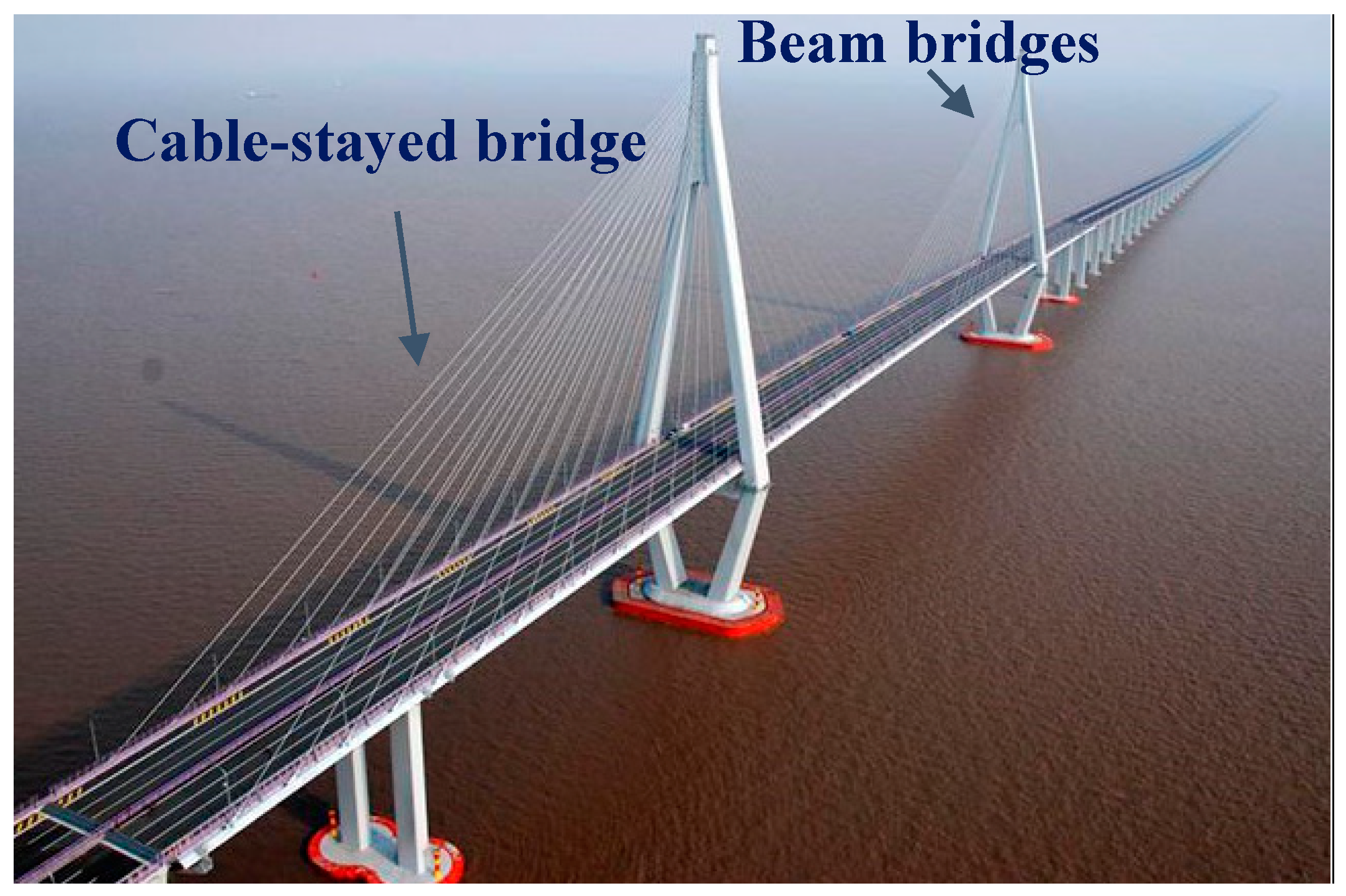
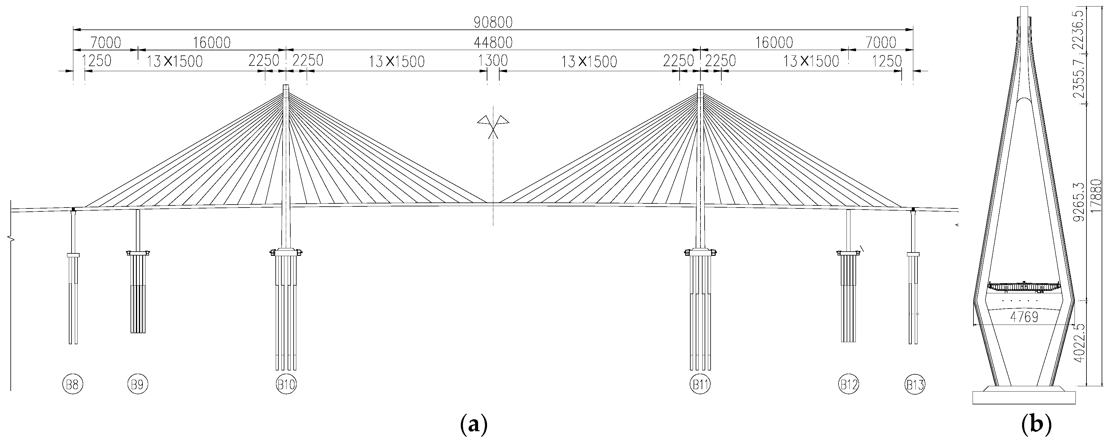
2. The Hangzhou Bay Cable-Stayed Bridge

2.1. Bridge Information

The Hangzhou Bay Bridge is a large-scale bridge across the Hangzhou Bay in the eastern coastal region of China with a total length of 36 km. It is among the ten longest trans-oceanic bridges in the world. The construction of this bridge was completed on 14 June 2007 and opened to traffic on 1 May 2008. It consists of a cable-stayed bridge with the main ship-channel and a large quantity of beam bridges (Figure 1). This cable-stayed bridge is selected for the ambient vibration measurement. In the following study, the Hangzhou Bay Bridge only refers to this cable-stayed bridge if not otherwise specified.
The Hangzhou Bay Bridge has one main span along with four side spans, each measuring 70 m, 160 m, 448 m, 160 m, and 70 m, as shown in Figure 2a. The connection between the girder and pylon is designed as a semi-floating system, which is beneficial to increasing the earthquake resistance at the limit stage. The side spans are additionally supported by the auxiliary piers in order to improve the dynamic behavior for daily service.
The pylon of the Hangzhou Bay Bridge is designed as a diamond-shaped structure, of which the height is 178.8 m from the base level to the top (Figure 2b) and 138.575 m from the girder. The cable system consists of 28 pairs of stay cables on each side of the pylon and is arranged in double-plane as a semi-fan shape. The minimum and maximum number of steel wires within a cable is 109 and 199, respectively. The main girder is primarily supported by the cable system and also sits on a transverse beam of the pylon. The flat steel box is applied as the girder’s cross-section 3.5 m high and 37.1 m wide (Figure 3). Inside the box girder, the steel crossbeams are added at a 3.75 m interval to improve the girder’s resistance to the torsion.

2.2. Soil Properties

Based on the boring information at the bridge site, 17 layers of soils numbered from the top to the bottom are categorized as eight types, including the cohesionless sand 1 (Layer 1, elevation: −9.9~−18.4 m), cohesive clay 1 (Layers 2~5 elevation: −18.4~−39.9 m), cohesionless sand 2 (Layers 6~8 elevation: −39.9~−71.1 m), cohesive clay 2 (Layers 9~10 elevation: −71.1~−84.0 m), silty fine sand 1 (Layer 11 elevation: −84.0~−96.5 m), cohesive clay 3 (Layers 12~15 elevation: −96.5~−120.8 m), silty fine sand 2 (Layer 16 elevation: −120.8~−139.8 m), and rounded gravel (Layer 17 elevation: deeper than −139.8 m). The bottom of the piles is located in the 7th category (silty fine sand 2), which is regarded as a good supporting layer for the foundation [45]. The soil parameters of each layer are tested by the bridge design company and the details are not provided here due to the page limit.

2.3. Potential Scour Development

The Hangzhou Bay Bridge is located in the Hangzhou Bay where the sea flow is rapid and turbulent and the tide is intensive. There are many suspended sediments floating with the current, and erosion and deposition occur very often along the seabed. Especially at the foundation of the bridge, the angle between the current direction and piers or pylons is large, resulting in a rapid removal of the soils. In addition, considering the bridge has served for almost ten years, the foundations of the bridge, especially at the pylons, may already have been scoured. In this sense, the Hangzhou Bay Bridge is appropriate as a case study subject to demonstrate the feasibility and convenience of the vibration-based scour identification in engineering practice.
The final balanced scour depths of the pylon are predicted by the solutions of different design specifications and water-tank experiments as listed in Table 1. It can be observed that the scouring of the Hangzhou Bay Bridge could be very critical during its service time.

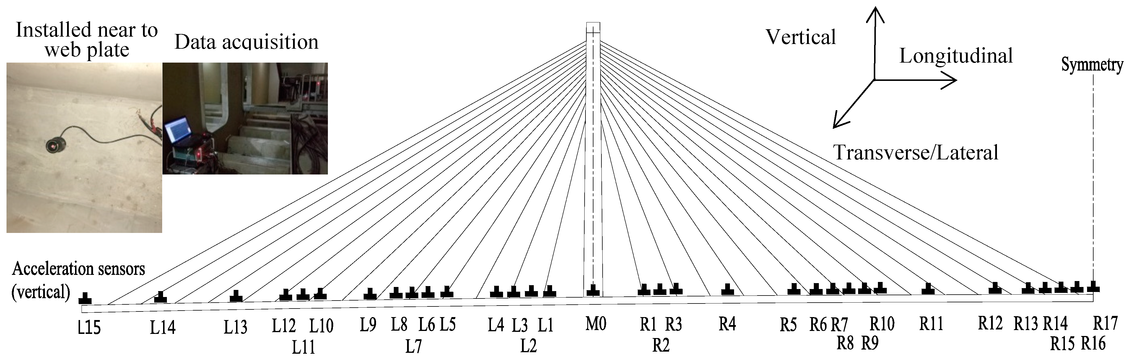
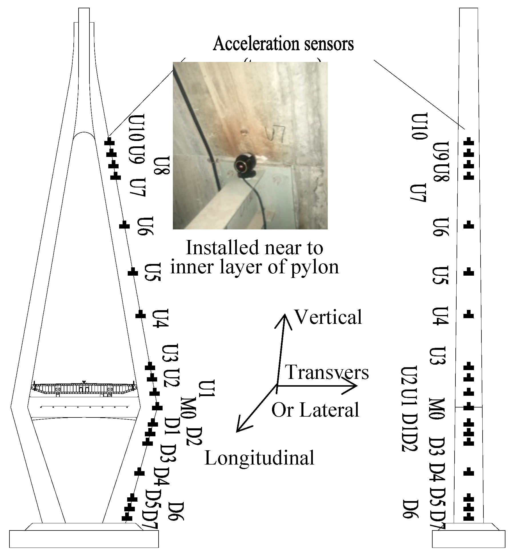
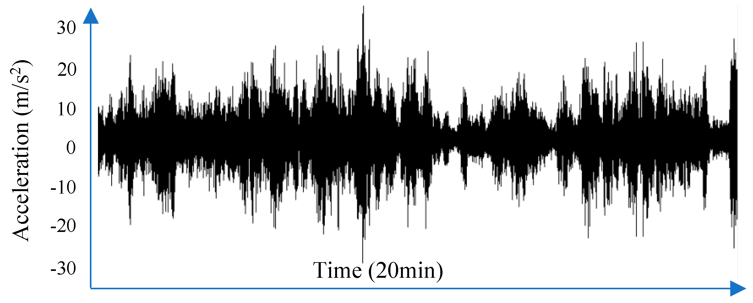
3. Ambient Vibration Measurements

Two ambient vibration measurements of the Hangzhou Bay Bridge were conducted in 2013 and 2016 to obtain its dynamic features. The field environmental forces, i.e., earth pulsation, hydrodynamic forces, or random traffic flow, excite the ambient vibration. The measurements covered the interior of the steel box girders at the main and side spans and the pylon structures above the pile cap. The sensors employed in the measurements were the broad-band acceleration-meters INV9828 from COINV (China Orient Institute of Noise & Vibration). The sensitivity of the sensors is 0.17–100 Hz with four gear selections and the resolution response is 0.0004 m/s2.
Based on the theory of modal analysis and structural characteristics of the bridge, the following locations were selected to install the sensors and ensure sufficient information measured from the vibration.
(1)
Locations at each wave crest and trough of the mode shapes. These mode shapes are the ones of low order and sensitive to the scour.
(2)
Locations at quartile division points between the adjacent crest and trough of the selected mode shape wave. The wave profile can be predicted by the FE method before the measurement.
(3)
Locations at the points with a significant change of mode shapes. More than four sensors are suggested to be sequentially installed to determine the curvature of the shape change.
(4)
Locations at the scour-sensitive components, such as the pylon and girder near piers.
(5)
Locations with the convenience of installation and measurement. For example, all the sensors were installed inside the steel box girder and the pylon of the Hangzhou Bay Bridge, as shown in Figure 4 and Figure 5.
(6)
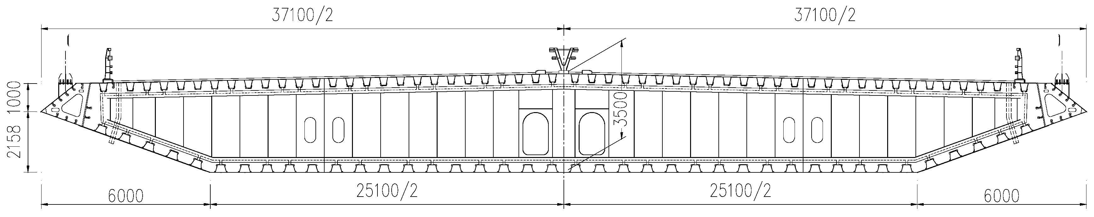
Locations at the components with few local vibrations, such as the web plate or crossbeams of the steel box girder, as shown in Figure 4.
(7)
Sensor installation needs to follow the direction of the vibration for each scour-sensitive mode shape. For example, the sensors for measuring the pylon needs to be installed horizontally since the scour-sensitive mode shapes of the pylon mainly vibrate transversely.
The final arrangements of the sensors are illustrated in Figure 4 and Figure 5 for the girder and pylon, respectively. The location of each sensor is denoted with a capital letter to categorize its position at different structural regions. L (L1-L15) and R (R1-R17) in Figure 4 denote the locations on the girder on the left and right sides of the pylon, respectively; U (U1-U10) and D (D1-D7) in Figure 5 denote the locations on the pylon above and below the girder, respectively. M (M0) in both Figure 4 and Figure 5 denote the intersecting location of the girder and pylon. All the letters are followed by different numbers to indicate their relative distances to the pylon or girder.
All the vibration measurements for the Hangzhou Bay Bridge were conducted under the ambient excitation without interrupting the traffic. A duration of 20 min was adopted for each time of recording with a sampling rate at 100 Hz. The measurements inside the steel box girder were targeted to the identification of the bending modes of the girder in the vertical direction. Horizontal direction was the target in the pylon case for its transverse bending modes. It is also noteworthy that the measurements need to be conducted by several subsequent steps with the common or shared reference points, i.e., M0, L1, and R1 for the girder and U6 and U7 for the pylon, due to the limited number of available sensors. Taking the reference point of M0 as an example, the acceleration signals recorded in the time domain from the sensor are provided in Figure 6.

4. Qualitative Scour Identification by Tracing Dynamic Features

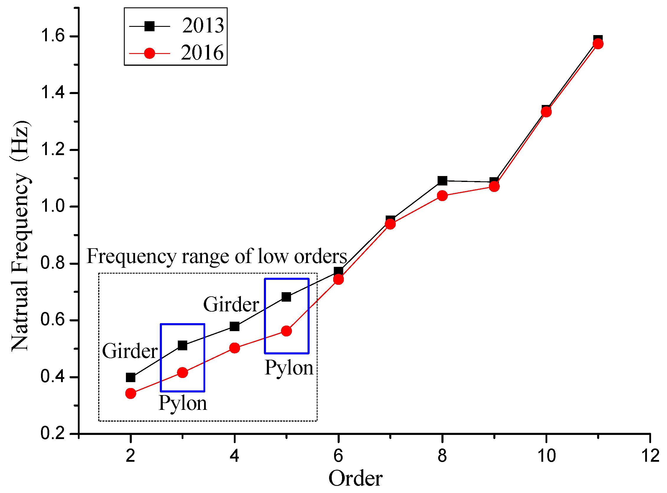
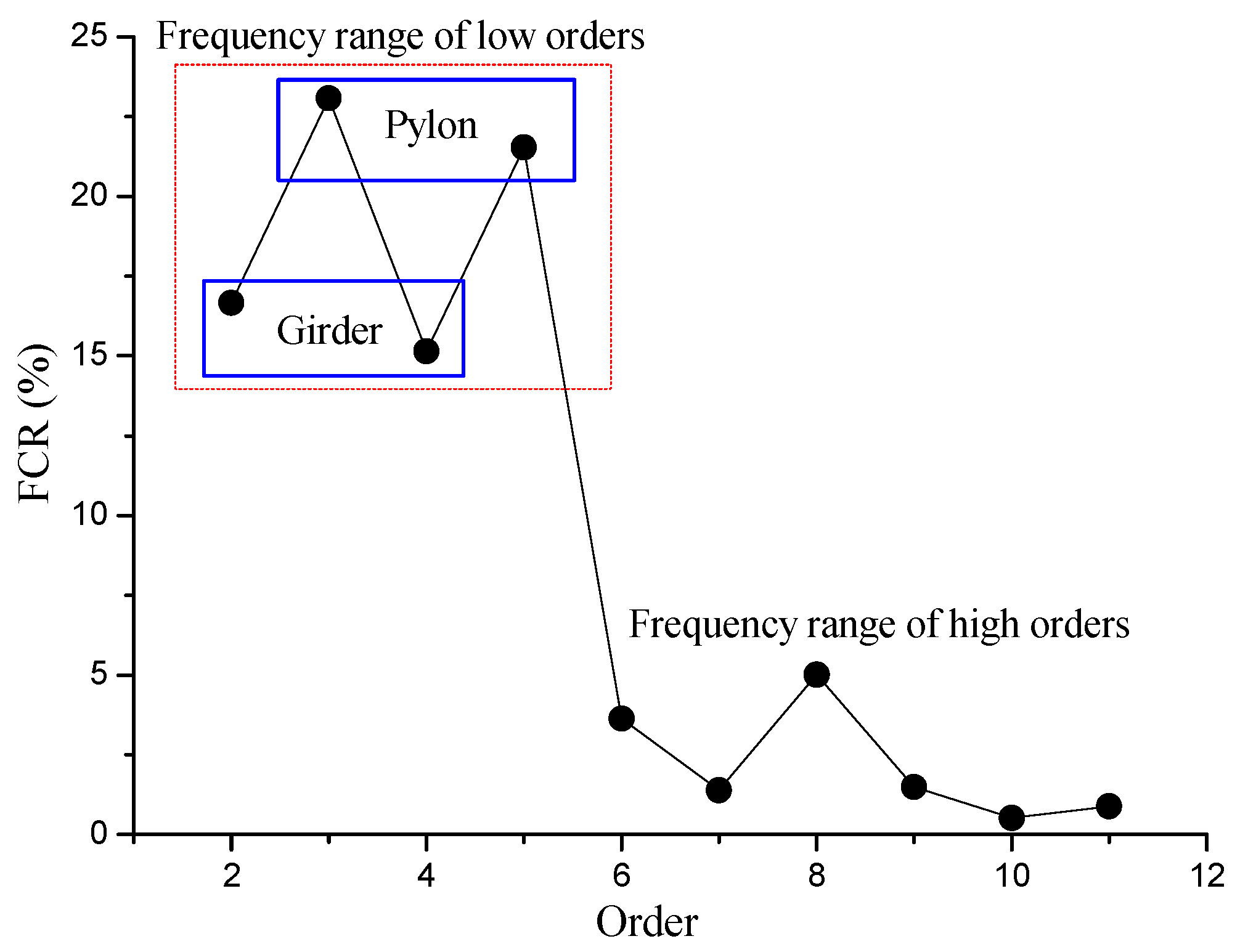
4.1. Identification by the Change of Natural Frequencies

The very high frequency components of the vibration signals measured in 2013 and 2016 were first removed by the wave filtering (low-pass wave filter) method to eliminate the vehicle-induced local vibration of the deck. Then, the modal analysis using the subspace iteration method was applied to the filtered vibration signals. In this way, the natural frequencies of the first eleven orders of the Hangzhou Bay Bridge were extracted from the two measurements and are provided in Table 2.
Comparing the extracted natural frequencies in the measurements of 2013 and 2016, a significant disparity can be clearly observed in Figure 7. In addition, the natural frequencies of almost all the orders decrease in 2016. The global frequency change should be mainly induced by the change of whole structural stiffness. For bridges, the whole structural stiffness can only be significantly influenced by the variation of the support boundary which in most cases is caused by the scour. In this sense, the natural frequency change of the superstructure has a strong relationship with the development of the foundation scour. The decrease of the natural frequencies from 2013 to 2016 shown in Figure 7 clearly indicates and qualitatively identifies the scour occurrence at the Hangzhou Bay Bridge.
It is also observed from Figure 7 that the frequency range of low orders from the 2nd to 5th, especially for the modes of the pylon, shows more distinguishable disparity between two measurements than other orders. This observation reveals that the natural frequencies of different orders or components have different sensitivities to the scour development (the variation of the support boundary). In order to describe the sensitivity, a new parameter of the frequency change ratio, abbreviated to “ F C R ” hereafter, is proposed as follows:
F C R = Δ ω ω
ω = the natural frequency; and Δ ω = the change of the natural frequency (absolute values).
Figure 8 shows the values of F C R corresponding to different orders of vibration modes based on the two measurements. The values of F C R are generally above the level of 15% for the orders from the 2nd to 5th while under the level of 5% for the high orders. This is because the low-order modes of vibration contribute to almost all the measured ambient vibration. Once the vibration is affected by the scour, the low-order modes should be influenced much more significantly than others. Especially for the low-order modes with the pylon (the 3rd and 5th orders), they have higher values of F C R (20–25%) than those with the girder (15–20%). Although the high-order modes yield the low values of F C R , a locally higher value of F C R (5%) still can be observed for the 8th mode with the pylon (1st anti-L (girder) + 2nd anti-L (pylon)) than the nearby modes (mostly lower than 1%). This is because the scour, which directly determines the support boundary of the pylon, has more significant effects on the pylon stiffness than that on the girder.

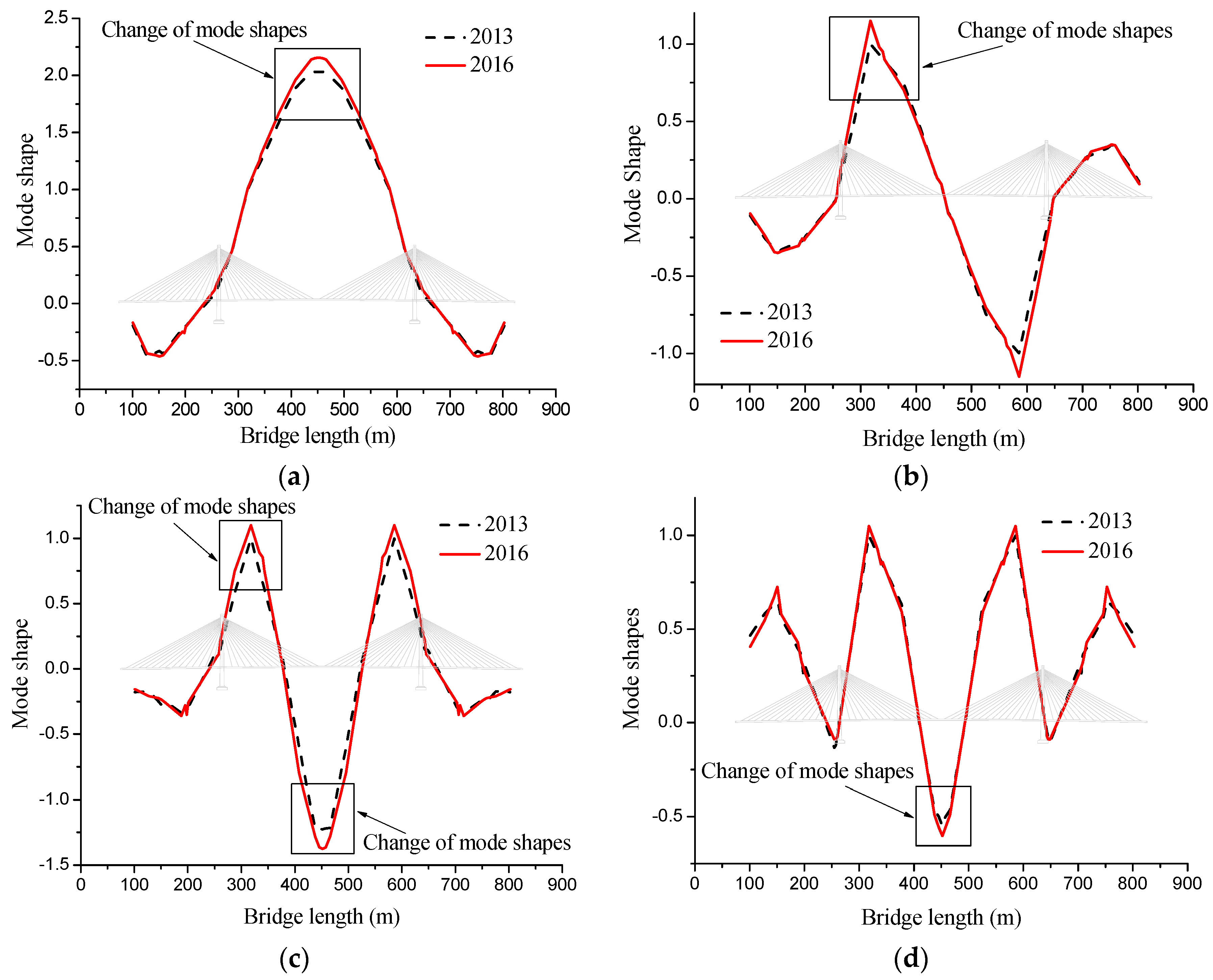
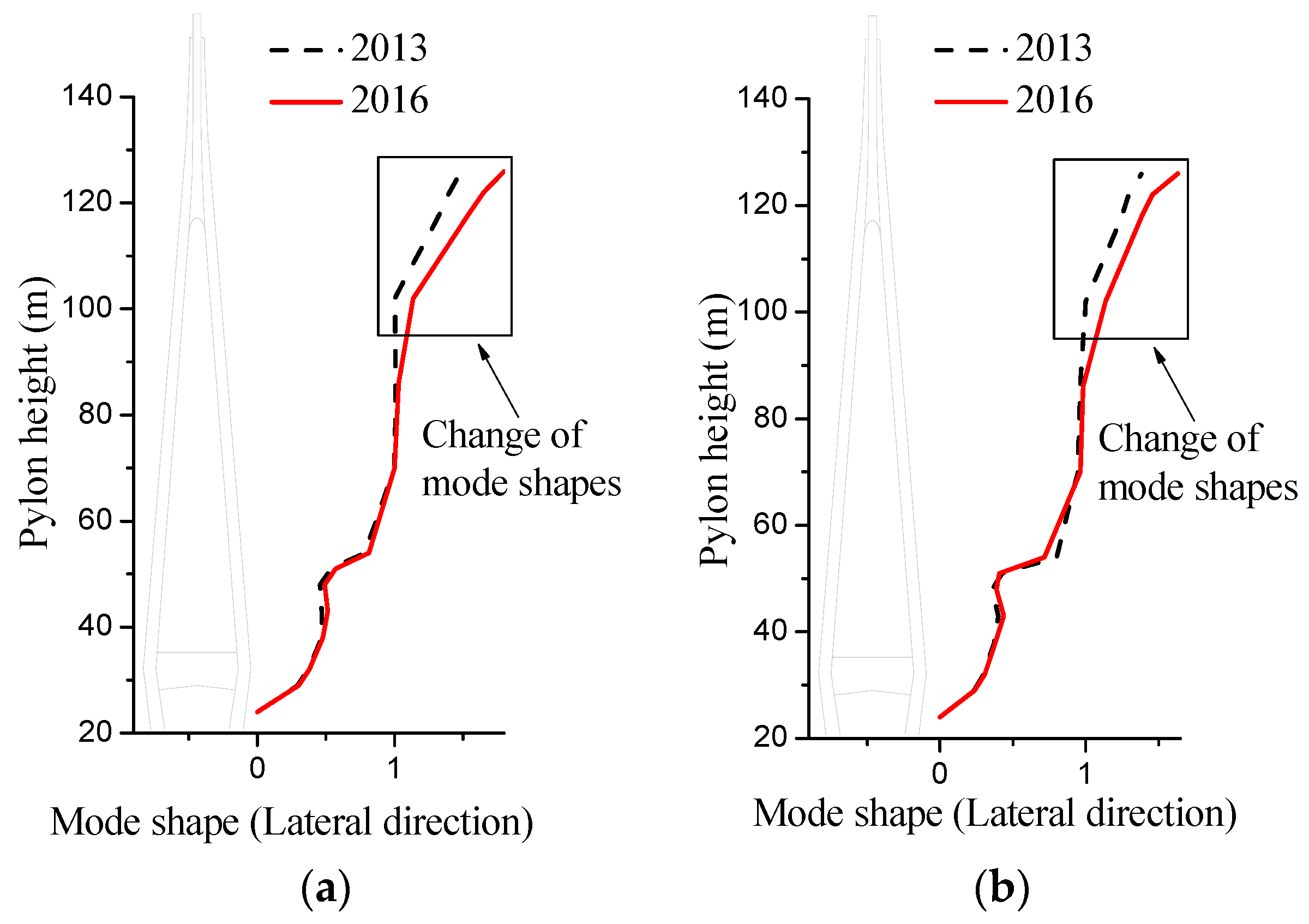
4.2. Identification by the Change of Mode Shapes

The mode shapes of the first eleven orders of the Hangzhou Bay Bridge were obtained using the subspace iteration method based on the ambient vibration measurements. Figure 9 compares four pairs of mode shapes of the girder which have the same order when extracted from the measurements of 2013 and 2016 (the shape scale was determined by the same normalization processing).
The significant changes of these mode shapes after three years are highlighted in Figure 9 in the rectangle. Most changes of the mode shapes occur locally at the vibration crests and troughs of the girder especially in the main span close to the span center and pylon. Such shape changes become more distinguishable if the order of the mode decreases. For example, the 1st mode in Figure 9a presents a much more distinguishable shape change than the 3rd mode in Figure 9d. It is also noticed that besides the significant local changes, the mode shapes also vary along the whole bridge length (908 m). This global difference in the mode shapes can be mainly attributed to different supporting boundaries of the bridge. It has been widely believed that the bridge scour is the most probable and usually physical explanation for the variation of the supporting boundary. In this sense, the change of the mode shapes of the girder, especially at their local crests and troughs, becomes another convincing indicator for the scouring of the Hangzhou Bay Bridge.
Similar shape changes can also be found by comparing mode shapes of the pylon which have the same order when extracted from the measurements of 2013 and 2016. The comparative results of the lateral bending modes of the pylon are provided in Figure 10 (the shape scale was determined by the same normalization processing), where the left figure is based on the mode that two pylons vibrate antisymmetrically and the right one is based on the symmetric mode. The unsmooth mode shapes in the figure are due to the limited number of the sensors installed in this case. It can be seen from both modes that the upper section of the pylon presents a much more significant shape change than the bottom part. The lower the order of the mode is, the more distinguishable the shape change between two measurements is. If comparing the results of Figure 10 to Figure 9, the pylon presents a more visible change of mode shapes between two measurements than the girder. This is because the pylon vibrates as a rigid rotation around the foundation and the scour depth directly determines the unsupported height of the pylon. Therefore, by tracing the change of mode shapes of the pylon, especially on the top sections, the change validates again the previous identification results for the scour of Hangzhou Bay Bridge.
Based on the analysis above, it can be concluded that: (1) the scour development of the Hangzhou Bay Bridge can be qualitatively identified by tracing the change of either natural frequencies or mode shapes between the measurements of 2013 and 2016; (2) the dynamic features of low orders are more sensitive to the scour than those of high orders; (3) the pylon presents more sensitive change of the dynamic features to the scour than the girder does, even for the high orders.

5. Quantitative Scour Identification by FE Model Updating

The change of pile-soil stiffness affects vibration modes by changing the restriction capacity provided by soils (such as fixed or joint connections). The change of scour depth affects vibration modes by changing the component length of foundations (pile, pier, or pylon). Considering the above different influential sources, all the vibration modes of bridges can be classified into two groups: scour-sensitive modes and scour-insensitive modes. Then, the quantitative scour identification was conducted in the following three steps: (1) First, an FE model was established as the object for the model updating; (2) Second, the soil stiffness (stiffness of soil-pile springs) was identified by model updating until the simulation results best fit the measurements of the scour-insensitive vibration modes. (3) Using the soil-updated model, the scour development was finally identified by model updating until the simulation results best fit the variation between two measurements of the scour-sensitive vibration modes. In the second step, the scour-insensitive vibration modes were used to update the values of soil stiffness. This is because all the global vibration modes of bridges should be influenced by different soil stiffness no matter if they are scour-sensitive or scour-insensitive. A similar phenomenon can also be found in the Kao-Ping-His cable-stayed bridge [7] and Jintang cable-stayed bridge whose frequencies of the scour-insensitive modes have 5% to 10% changes when the pile-soil stiffness increases by 75%.

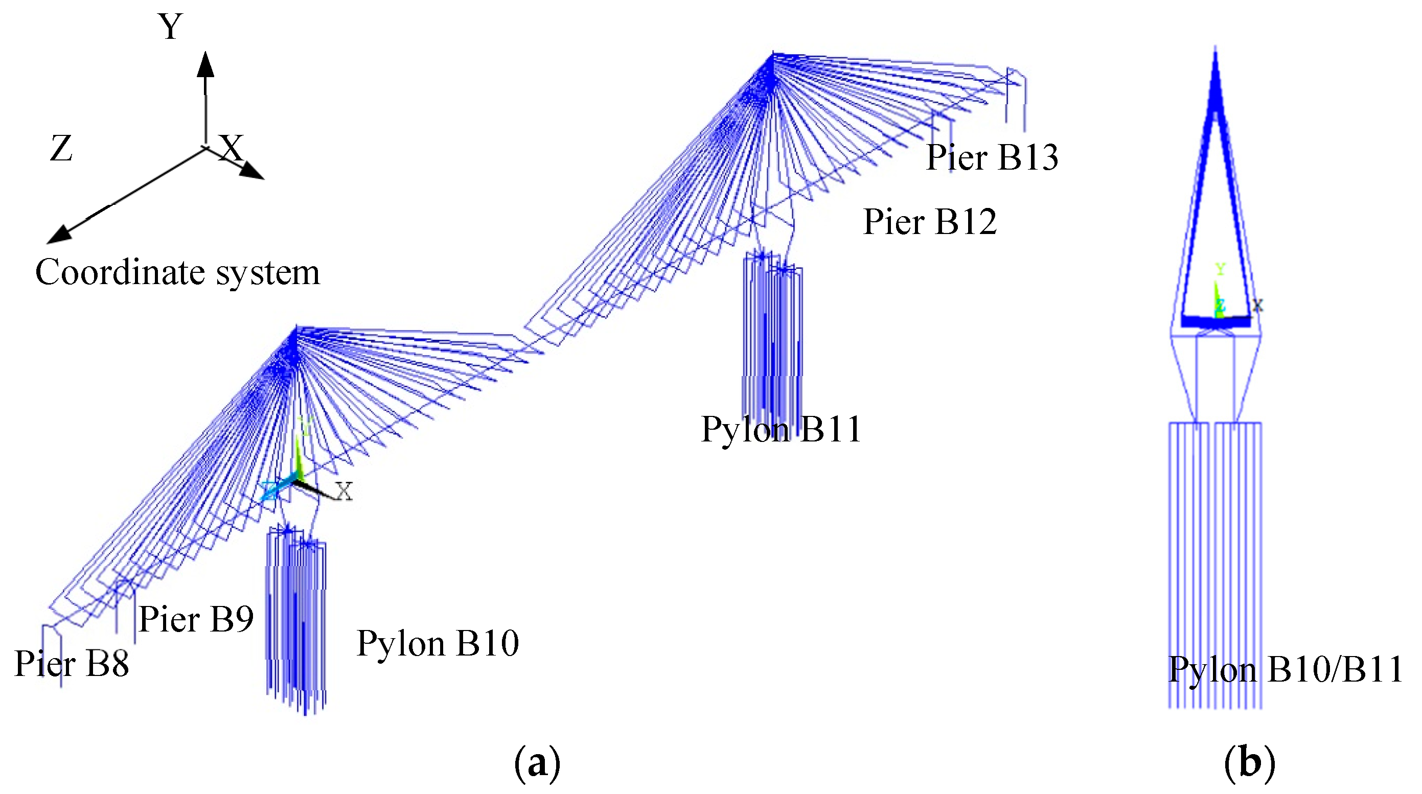
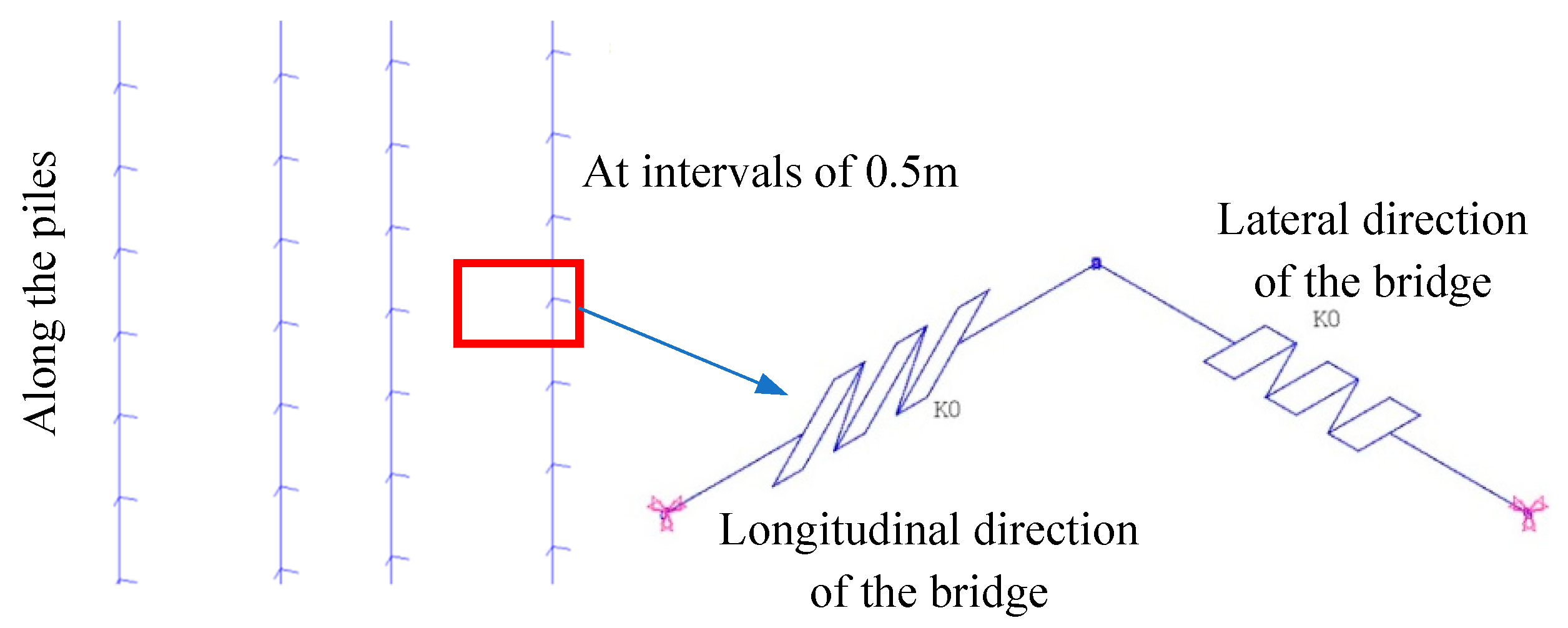
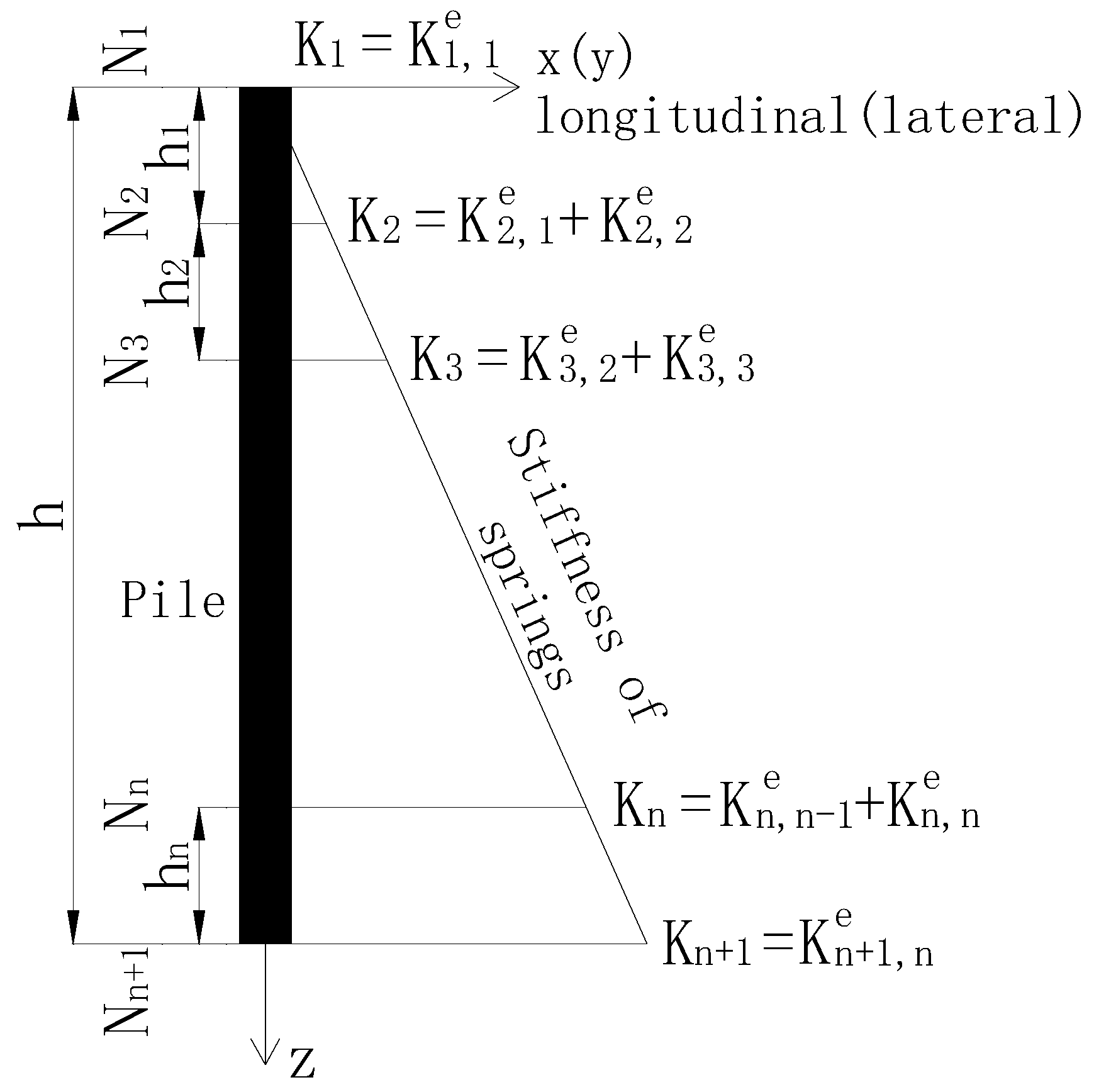
5.1. FE Model Establishment

Based on the engineering drawings of the Hangzhou Bay Bridge, a 3D Finite Element (FE) model was created using the ANSYS program. A fish-bone structural system was selected to model the superstructure which can accurately simulate the stiffness of cable-stayed bridges by using beam elements (Figure 11) [47]. In the model, the main girder was simulated by a longitudinal single beam, i.e., Beam188 element, with all the material properties referring to the detailed design parameters. The Beam188 element has three translational and three rotational degrees-of-freedom (DOFs) for each node. The crossbeams intersected with the main girder were modeled by transverse beams using the same Beam188 element. The torsional moments of inertia of crossbeams were considered by the Mass21 element. All the stayed cables connected to the ends of crossbeams were modeled by the Link8 element with the consideration of the existing cable forces. The Link8 element has two translational DOFs for each node. The pylons were also modeled using the Beam188 element to reduce the computation effort. The cross sectional configurations and material properties for each component of the FE model are listed in Table 3 and Table 4, respectively. The densities of the girder and cross beams were re-calculated after accounting for all the stiffening and non-structural components.
The key issue to establish the FE model of a scoured bridge is the pile-soil interaction and the corresponding effective area. Soil behavior is highly nonlinear and in particular its stiffness changes nonlinearly with the strain. The response of the pile-soil system is heavily dependent on the magnitude and type of external loads. However, in the service stage of bridges, the external loads over the bridge will only lead to a very small lateral strain being imparted into the soil surround the piles. Therefore, for the case of the Hangzhou Bay Bridge, it is assumed that the soil strains remain within the “small-strain” linear-elastic region of the soil response curve.
In the present study, the pile-soil interaction was represented by the stiffness of soils. All the soil layers in the FE model were simulated by the discrete and closed spaced spring elements (Combin14) at intervals of 0.5 m along the piles (Figure 12). The spring element of the Combin14 with a null mass matrix has two translational DOFs (degrees of freedom) and allows one-dimensional uniaxial movement along the axis of the spring. Each node of the pile connects two spring elements along the longitudinal and lateral directions of the bridge. For the purpose of dynamic interaction modeling, the springs are assumed to provide dynamic impedance only and inertial effects are ignored. Then, an appropriate determination of the element stiffness of the springs becomes the next pursuit, which plays a very important role in the soil behavior simulation.
According to the one-parameter Winkler soil model for piles, the lateral resistance of soils on the pile at a certain depth is linearly varied with the increase of the lateral displacement of the pile. This linear elastic expression is provided by the following mathematical equation.
σ z = C u z
where σ z = lateral resistance of soils on the pile at the depth of z (kN/m2); u z = lateral displacement of the pile at the depth of z (m); and C = foundation coefficient (KN/m3), which is usually a function of the depth (Equation (3)).
C = k z n
where k = coefficient related to the soil types, mechanical parameters, material properties, depth, etc.; z = soil depth; and n = exponent of z. Further assigning n a value of 1.0 in the present study yields Equation (4), a simplified Winkler-based relationship between C and z.
C = m × z
where m = coefficient (kN/m4),; its value can be found in the foundation design specifications of different countries. Considering that the Hangzhou Bay Bridge is located in China, the Chinese code for the design of the ground base and foundation of highway bridges and culverts (JTG D63-2007) was selected in the present study to specify the value of m.
Since the spring elements were modeled discretely at intervals of 0.5 m, Equation (4) as a continuous relationship between C and z cannot be directly applied to determine the stiffness of each spring. Therefore, the lateral resistance of soils between two close-by springs needs to be equivalently converted into two nodal forces at the nodes of the springs. Such equivalence between a continuous soil force and two discrete nodal spring forces was achieved by keeping the lateral restrain and bending moment of the pile the same. The specific conversion process of the lateral forces on the pile involves the following steps and the result is applicable to both the longitudinal and lateral springs.
Step (1): The pile embedded in the soil is divided into n elements from the top to bottom. The length of each pile element is hj (j = 1, 2, …, n) and two nodes of the jth element are Nj and Nj+1, as shown in Figure 13.
Step (2): Based on Equation (4), the stiffness distribution of soils along the pile forms a triangle shape starting from the top of the pile embedded in soils. Then, according to the equivalence principle specified earlier, the stiffness of discrete springs at the nodes N1 and N2 can be derived as:
K 1 , 1 e = K ( h 1 ) × h 1 2 × 1 3 = K ( h 1 ) × h 1 6
K 2 , 1 e = K ( h 1 ) × h 1 2 × 2 3 = K ( h 1 ) × h 1 3
where K 1 , 1 e and K 2 , 1 e = stiffness of springs at the nodes N1 and N2 of the 1st element, respectively; and K ( h 1 ) = stiffness of soils at the depth h1 based on Equation (4), which is calculated as:
K ( h 1 ) = b 0 × m × h 1
where b0 = width of the pile.
Similarly, the stiffness of springs at the nodes Nj and Nj+1 of the jth element (j > 1) can be derived as:
K j , j e = K ( i = 1 j h i ) × h j 2 + [ K ( i = 1 j + 1 h i ) K ( i = 1 j h i ) ] × h j 6
K j + 1 , j e = K ( i = 1 j h i ) × h j 2 + [ K ( i = 1 j + 1 h i ) K ( i = 1 j h i ) ] × h j 3
where K j , j e and K j , j + 1 e = stiffness of springs at the nodes Nj and Nj+1 of the jth element, respectively; and K ( i = 1 j h i ) and K ( i = 1 j + 1 h i ) = stiffness of soils at the depths i = 1 j h i and i = 1 j + 1 h i , respectively, which based on Equation (4) are calculated as:
K ( i = 1 j h i ) = b 0 × m × i = 1 j h i
K ( i = 1 j + 1 h i ) = b 0 × m × i = 1 j + 1 h i
Step (3): Since one node connects two elements, the stiffness of the spring at each node (Dexcept node N1) should add up to the contributions from both connecting elements (Figure 13). Therefore, the stiffness of all the springs in the FE model can be assigned by the values based on the following equation.
K 1 = K 1 , 1 e K 2 = K 2 , 1 e + K 2 , 2 e K n = K n , n 1 e + K n , n e K n + 1 = K n + 1 , n e

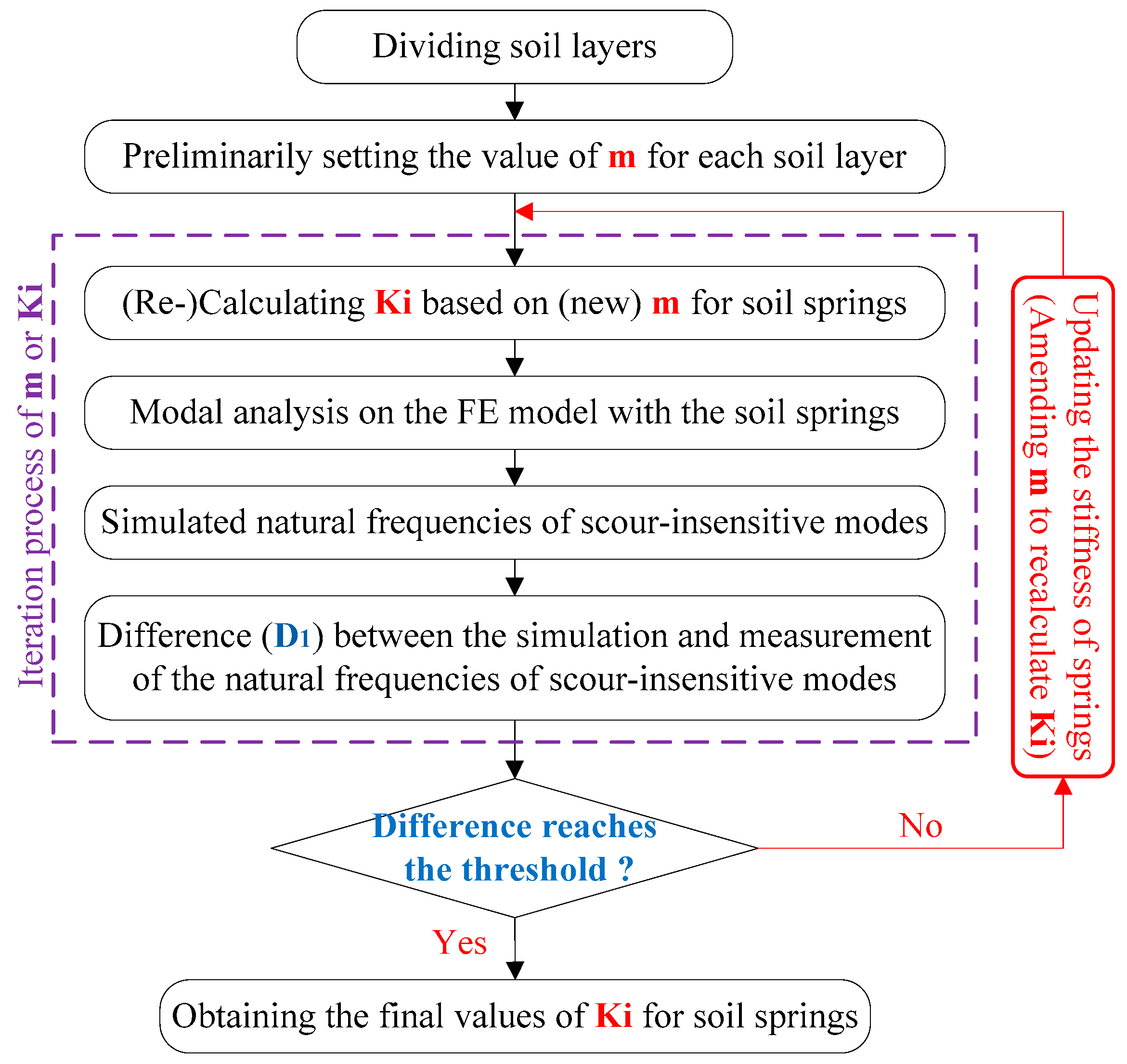
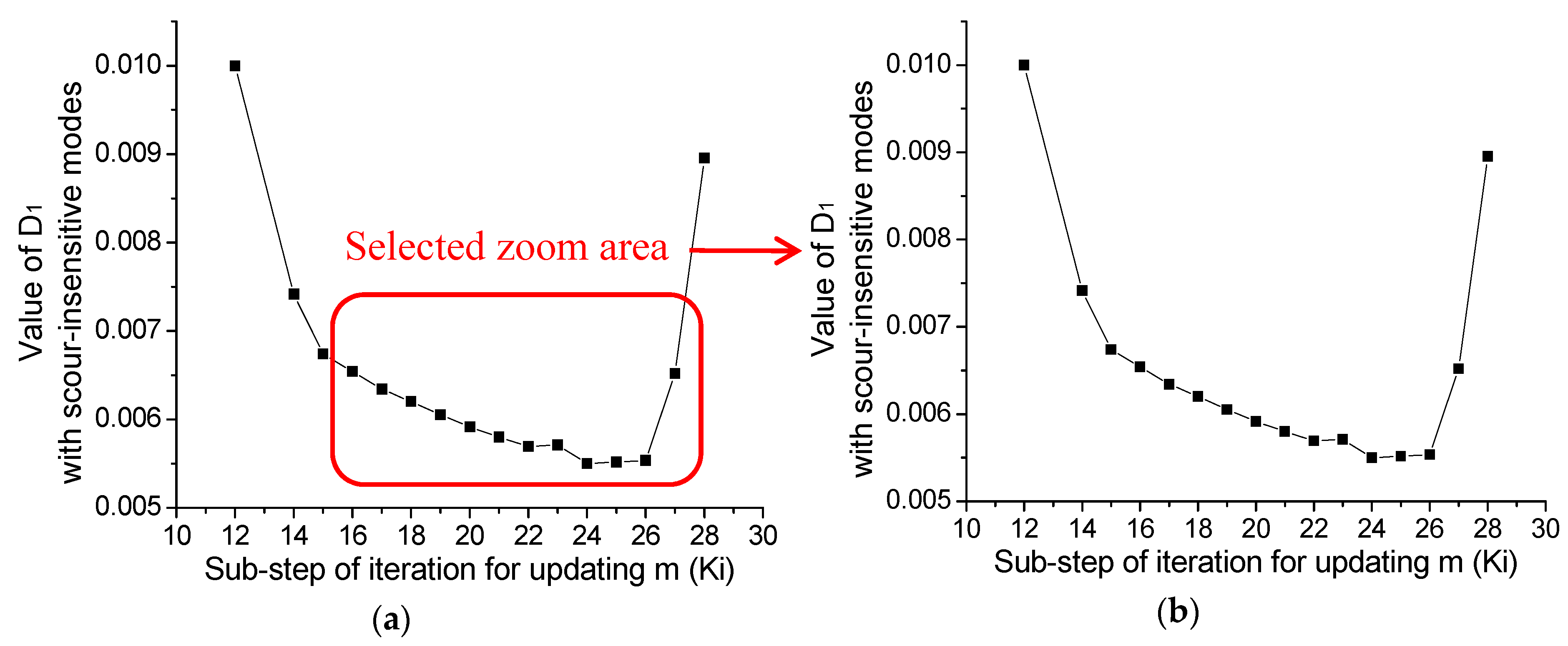
5.2. Identification of Soil Stiffness

The above theoretical derivation provides the preliminary values for the stiffness of soils/springs (Ki). These Ki values need a further identification based on field measurements to best fit the actual response of the Hangzhou Bay Bridge. Based on Figure 8 and the corresponding discussion, the 6th, 7th, 9th, 10th, and 11th vibration modes have the indicator of F C R less than 5%, which shows that the natural frequencies of these modes are negligibly affected by the scouring between two measurements. In other words, the 6th, 7th, 9th, 10th, and 11th vibration modes are insensitive to the scour. The stiffness of soils/springs (Ki) becomes the last main reason to affect the natural frequencies of these five modes. Therefore, the real values of Ki for all the springs in the FE model can be identified by model updating until the simulated natural frequencies of the scour-insensitive vibration modes match the measurements. The adoption of scour-insensitive vibration modes significantly lowers the scour interference during the model updating of soil stiffness. This mode sensitivity can also be determined by the FE simulation of the bridge if there is not enough information from field measurements. By the parametric study based on the FE model, a scour-sensitive vibration mode still remains sensitive when the scour keeps developing. Considering Ki is a function of the coefficient of m based on Equations (4)–(12); the algorithm for identifying soil/spring stiffness by amending m to update the values of Ki is provided in Figure 14.
Following the algorithm, the foundation soils of the Hangzhou Bay Bridge were first divided into eleven different layers according to the geological survey results. Since the bridge is located in China, all the soil layers were assigned with initial values of m based on the Chinese code for design of ground base and foundation of highway bridges and culverts (JTG D63-2007), as listed in Table 5. The stiffness of soil springs in the FE model with these initial values of m was accordingly calculated by Equations (4)–(12). By using this FE model, the simulated natural frequencies of different orders of the bridge were numerically obtained.
In order to quantitatively describe the difference between the simulated and measured natural frequencies, a new parameter is proposed in Equation (13).
D 1 = q ( f s i m q f m e a q ) 2
where D1 = difference between the simulated and measured natural frequencies; f s i m q and f m e a q = simulated and measured natural frequencies of the qth vibration mode, respectively; and q = concerned orders, which refer to the orders of the scour-insensitive vibration modes. It is noted that other forms of D1, i.e., Root-Mean-Squared-Error (RMSE) and the Nash-Sutcliffe Efficiency, can also be used in Equation (13), which should provide the same iteration results.
If D1 is greater than a preset threshold, m for each soil layer needs to be further amended. Meanwhile, the natural frequencies need to be re-simulated based on the FE model with the newly amended m and accordingly a new D1 can also be calculated. This iteration process for updating the value of m (stiffness of springs Ki) is repeated until the value of D1 reaches the threshold.
For the Hangzhou Bay Bridge, the orders of the scour-insensitive vibration modes are the 6th, 7th, 9th, 10th, and 11th. Considering the soil stiffness barely changes, either the measurements in 2013 or 2016 can be selected as the data of modal analysis to calculate D1. The threshold of terminating the iteration is set as reaching the lowest value of D1 during the updating process. The stiffness of each soil layer keeps being updated by revising the value of m at intervals of 100 kN/m4 per sub-step of the iteration. The values of D1 calculated by Equation (13) at all the sub-steps of the iteration are provided in Figure 15.
Based on Figure 15, and especially the selected results in Figure 15b, the value of D1 keeps decreasing until the 24th sub-step of the iteration when it increases again. At this sub-step the difference between the simulated and measured natural frequencies of the 6th, 7th, 9th, 10th, and 11th vibration modes reaches its minimum during the entire iteration process. In other words, the pile-soil simulation in the FE model gradually approaches the actual situation of the bridge before this sub-step. Table 6 lists the values of m based on the results at the 24th sub-step of the iteration. Substituting the newly updated m into Equations (4)–(12), the new stiffness of soil springs Ki was subsequently obtained and then correspondingly updated in the FE model of the bridge. The updated values of Ki are listed in Table 7.
So far, the soil stiffness (stiffness of soil-pile springs) of the Hangzhou Bay Bridge was identified by best fitting the scour-insensitive vibration modes and accordingly updating the FE model. This updated FE model will be used in the following study as a reference model to further quantitatively identify the scour depth. It should also be noted that even if the soil stiffness is not identified accurately enough, the scour depth increasing is still the most significant reason for the change of vibration modes since the soil property hardly changes during the bridge service.

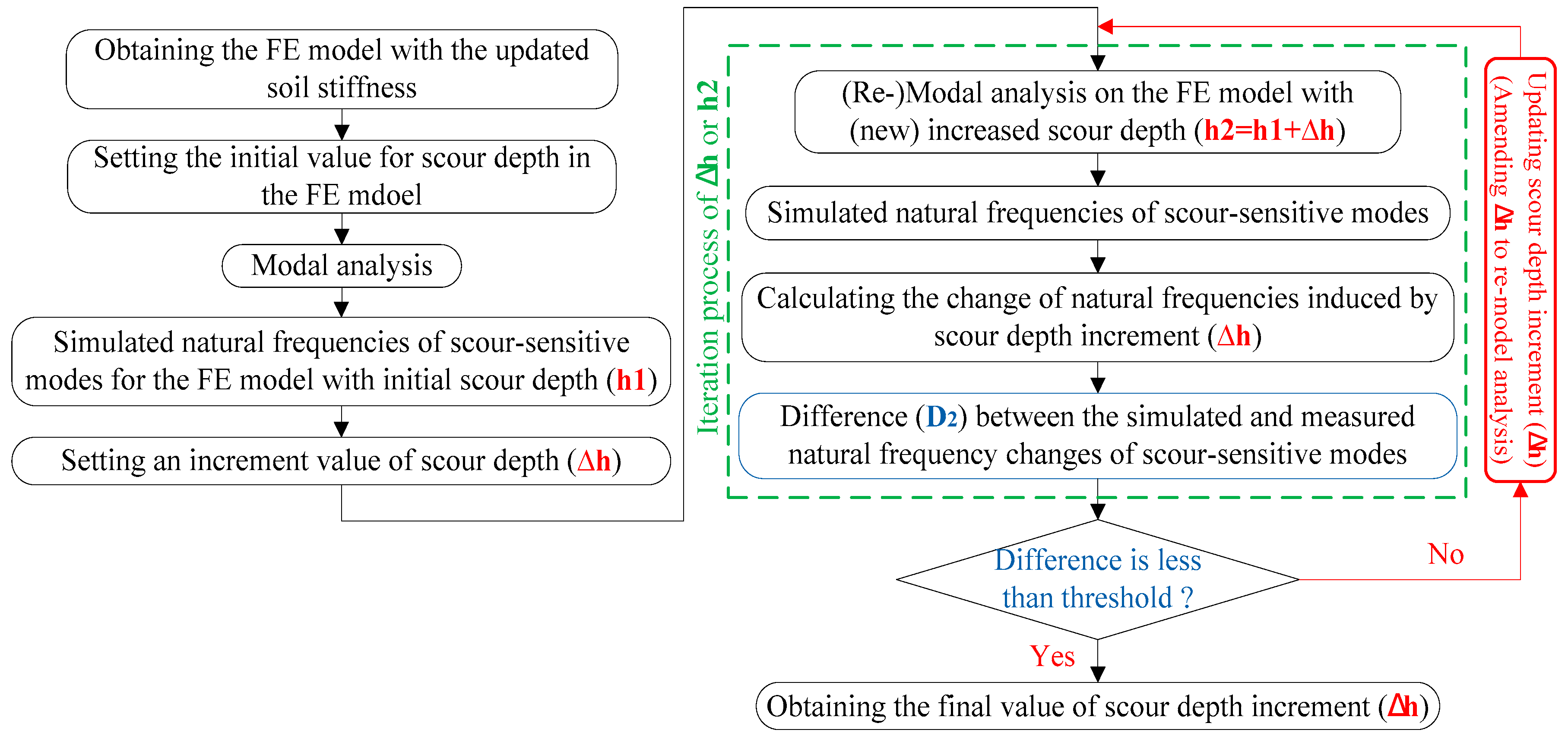
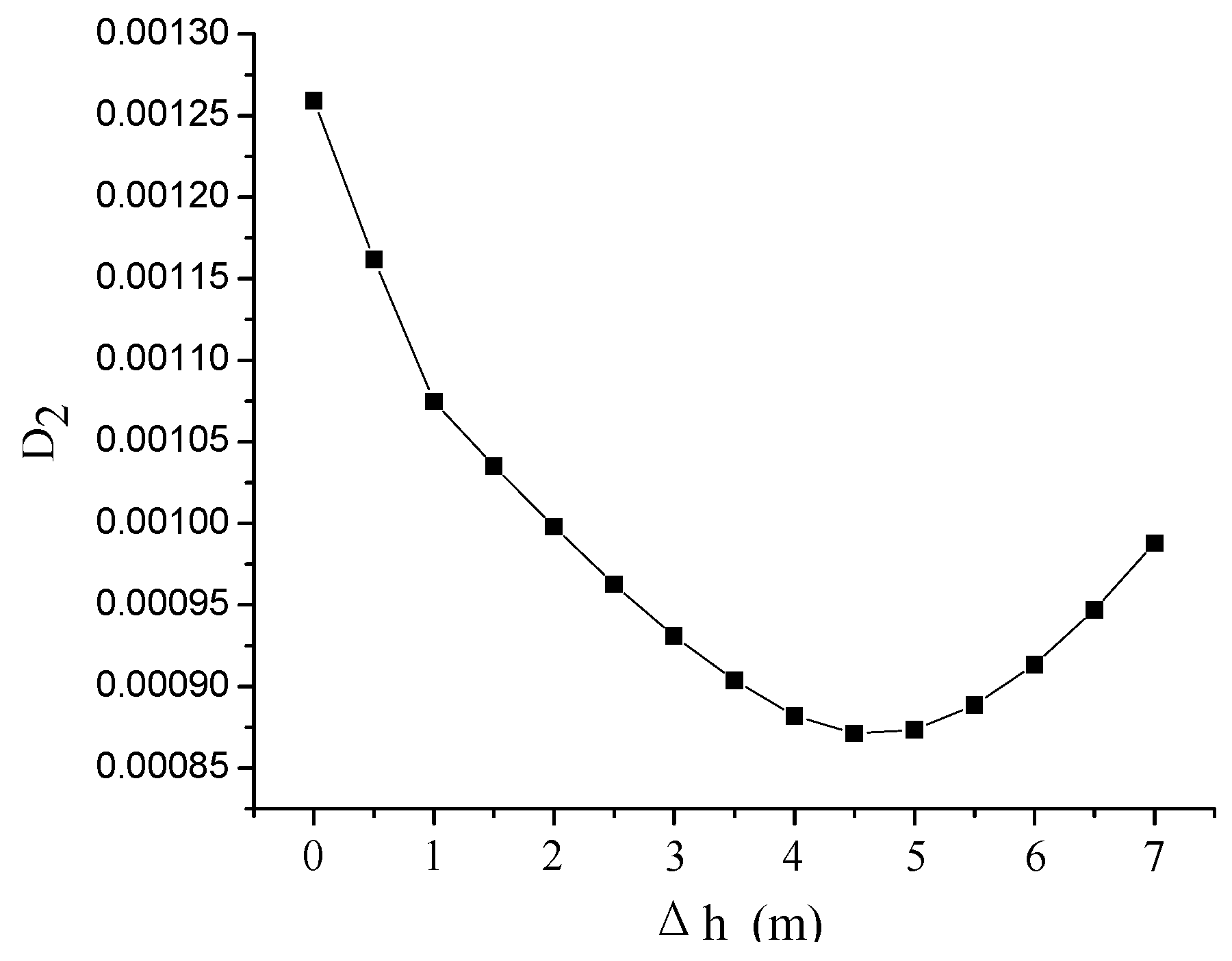
5.3. Identification of Scour Depth (Soil Level)

Considering there is no significant damage reported by the routine inspections on the superstructures of the Hangzhou Bay Bridge, the scour development should be the only reason for the variation of the dynamic features of the bridge. Therefore, in this case the scour depth was identified by updating the previous soil-updated FE model to best fit the measured natural frequency change from 2013 to 2016. Different from the soil updating, the scour-sensitive vibration modes were selected as the best fitting objects to update the scour depth. Using the scour-sensitive vibration modes can include the most scour effects on the variation of natural frequencies. In this way, the interference of other factors can be lowered to the maximum extent during the model updating of the scour depth. The algorithm for identifying the scour depth by model updating is provided in Figure 16.
Another parameter D2 is proposed in Equation (14) to quantitatively describe the difference between the simulated and measured natural frequency changes of scour-sensitive vibration modes.
D 2 = p [ ( f s i m , ( h 1 + Δ h ) p f s i m , h 1 p ) ( f m e a , 2016 p f m e a , 2013 p ) ] 2
where D2 = difference between the simulated and measured natural frequency changes; f s i m , ( h 1 + Δ h ) p = simulated natural frequency of the pth vibration mode by the FE model with the scour depth of h1 + Δh, i.e., h2; f s i m , h 1 p = simulated natural frequency of the pth vibration mode by the FE model with the scour depth of h1; f s i m , ( h 1 + Δ h ) p f s i m , h 1 p = simulated natural frequency change induced by the increment of scour depth Δh; f m e a , 2016 p = measured natural frequency of the pth vibration mode in 2016; f m e a , 2013 p = measured natural frequency of the pth vibration mode in 2013; f m e a , 2016 p f m e a , 2013 p = measured natural frequency change induced by the increment of scour depth from 2013 to 2016; and p = the orders of the scour-sensitive vibration modes.
For the Hangzhou Bay Bridge, the scour-sensitive vibration modes are the 2nd, 3rd, 4th, and 5th modes with more than 15% F C R based on Figure 8. The initial value of scour depth h1 set in the FE model before updating Δh was determined based on the underwater inspection report in 2013. The Δh was amended at intervals of 0.5 m per sub-step of the iteration until the D2 was less than the pre-set threshold. Subsequently, new natural frequencies were simulated based on the FE model with the newly amended Δh and a new D2 was also obtained. The threshold for terminating the iteration is set as reaching the lowest value of D2. The values of D2 calculated by Equation (14) at all the sub-steps of the iteration are provided in Table 8. Figure 17 plots the variation of D2 along with increasing Δh from 0 m to 7 m.
As can be seen from Figure 17, the D2 decreases with the progressive scouring until the Δh reaches the increment of 4.5 m. Thereafter, the D2 turns to increase as the Δh continues going deeper. In other words, the lowest value of D2 is obtained at the 10th sub-step of the iteration when the Δh is 4.5 m. At this moment, the difference between the simulated and measured natural frequency changes of the 2nd, 3rd, 4th, and 5th vibration modes reaches its minimum value. Therefore, the scouring of the Hangzhou Bay Bridge from 2013 to 2016 was successfully identified as the increment of 4.5 m. It is clearly observed from Table 9 that after model updating the frequency changes by adding 4.5 m scour depth in the FE model, which is very close to the measured changes. The proposed scour identification method worked very well in the present case study.

6. Verification by Results from Underwater Terrain Map

In this section, the documented results from the underwater terrain map were used to verify the accuracy of the scour identification by the proposed method based on the ambient vibration measurements.
Since a 6 m-deep local scour hole was observed at the Hangzhou Bay Bridge, an underwater terrain scanning measurement was conducted every year. A multiple-wave depth survey system called “Atlas FanSweep20 (FS20)” was applied for the scanning, which included the depth measurement meter, global navigation satellite system (GNSS) receiver, sound velocity meter, differential global positioning system (DGPS) device, acoustic doppler current profiler (ADCP), electronic total station, and survey boat. Each scanning can draw a digitized underwater terrain map for the region around the Hangzhou Bay Bridge, as shown in Figure 18. The scour developments can be quantitatively obtained by comparing the scanning results between different years. By doing this, Table 10 lists the increments of the scour depths from 2013 to 2016 at the side pier (B9) and pylon (B10) [6]. It should be noted that all the elevation values in Table 10 were measured in the deepest positions of the local scour holes. To make sure the underwater scan results and the vibration-based identification results are comparable, the months of conducting the vibration measurements in 2013 and 2016 were selected according to the time of the underwater scan.
An obvious scour development can be observed from Table 10 at either the side pier or pylon during the time from 2013 to 2016. The maximum increment was 5.2 m, locally located at the pylon B10, which was very similar to the above identified scouring of 4.5 m. The disparity between the identification by the superstructure vibrations and the result by the direct underwater measurements is only 13%. If considering the scouring of 5.2 m could include the interference of sediment refilling in scour holes, the real scour development at the pylon should be less than 5.2 m. Moreover, the scour may quickly vary in a very short-term period even though the underwater scan and vibration measurements were conducted in the same season. That is also one of the possible reasons for the disparity (4.5 m versus 5.2 m). Therefore, it was verified that the proposed method by the ambient vibrations of the superstructure can assure an accurate and quantitative result for the practical scour identification.
Although the dynamic nature of live bed scour condition (erosion and refilling) would continuously change the underwater scanning results of scour over time, it is actually not significant compared to the final scour depths and total lengths of piles. Such a measuring difference from real scour depths should only result in slight influence on the assessment of bridge safety and stability. Moreover, only the underwater terrain measurements were conducted as the yearly routine scour inspection for the Hangzhou Bay Bridge. Therefore, using the data from the underwater terrain measurements becomes the best choice at present to verify the accuracy of the proposed method.
In addition to the good accuracy, the proposed method only needs to trace the vibration signals of the superstructure without any underwater operations or devices. The acceleration sensors on the superstructure and their signal receiver are the only instruments installed during the identification. By doing this, the common issues of traditional scour inspections can be well avoided or solved, such as the high expense of operations, high maintenance of devices, and difficulty of long-term and high-frequency assessments. Therefore, this vibration-based scour identification could be easily integrated to a routine and long-term assessment task for bridges.

7. Concluding Remarks

This study shows the great potential for the use of the ambient vibration of the superstructure in identifying the bridge scour. The improvements in the present study compared to other existing studies are concluded from following two aspects.
(1)
Methodology improvements: In this study, the variation of mode shapes is incorporated to qualitatively detect the existence of bridge foundation scour, and a new two-step scour identification method was also proposed. By this method the scour is quantitatively identified by best fitting the scour-sensitive vibration modes (the 2nd step) using an FE model whose soil stiffness is pre-updated by best fitting the scour-insensitive modes (the 1st step).
(2)
Application improvements: The Hangzhou Bay Bridge, a 908 m cable-stayed bridge, was selected as a case study to comprehensively illustrate the application of this method. Another successful field application is important for this vibration-based scour identification method, which presently happens to significantly lack application for real bridges.
The following conclusions can also be drawn.
(1)
The high-order vibration modes are insensitive to the scour. The low-order vibration modes, especially for the modes of pylon, are very sensitive to the scour. Therefore, the natural frequencies of high and low vibration modes can be used as the tracing targets for updating the soil stiffness and scour depth.
(2)
The documented results from the underwater terrain map verify the accuracy of the proposed scour identification based on the ambient vibration measurements.
(3)
The proposed qualitative identification method can also be used to narrow down the number of bridges in need of further evaluation, e.g., the quantitative identification. It is noted that the quantitative identification needs enough bridge information to conduct the model updating. Both the qualitative and quantitative identification methods were suggested to be applied accordingly.
(4)
Once applied in practice, this vibration-based scour identification does not require any underwater devices and operations and could be easily integrated to a routine assessment task for bridges.
While the current research led to several new and interesting conclusions regarding the application of identifying bridge scour based on the ambient vibrations of the superstructure, additional research would also be beneficial. For example, the reliability in the practice of this method needs more validations, especially when other local damages besides the foundation scour pre-exist in the superstructure. Since the measurements of vibration modes (e.g., scour-sensitive and -insensitive) significantly affect the accuracy of the identification, an investigation on effective arrangement of sensors is also needed. More applications on different types of bridges are still required to fully confirm the applicability of the proposed vibration-based method.

Author Contributions

W.X. managed the whole research plan, took care all the data analysis, and did the manuscript writing. C.S.C. did the quantitative scour identification and model updating. B.K. did part of the simulation and the corresponding data analysis. X.Z. provided some of the original data. P.T. did the qualitative scour identification analysis.

Funding

This research was funded by the Natural Science Foundation of Jiangsu Province of China (grant number BK20161417), Fundamental Research Funds for the Central Universities (grant number 2242016R30023), and Highway Science and Technology Project of Zhejiang Province of China (grant number 2018H10).

Acknowledgments

The financial support for this work from the Natural Science Foundation of Jiangsu Province of China (Project No. BK20161417), Fundamental Research Funds for the Central Universities (2242016R30023), and Highway Science and Technology Project of Zhejiang Province of China (2018H10) is gratefully acknowledged. The opinions and statements do not necessarily represent those of the sponsors.

Conflicts of Interest

The authors declare no conflict of interest.

References

  1. Chen, G.; Schafer, B.; Lin, Z.; Huang, Y.; Suaznabar, O.; Shen, J. Real-time monitoring of bridge scour with magnetic field strength measurement. In Proceedings of the Transportation Research Board 92nd Annual Meeting, Washington, DC, USA, 13–17 January 2013. [Google Scholar]
  2. Wardhana, K.; Hadipriono, F.C. Analysis of recent bridge failures in the United States. J. Perform. Constr. Facil. 2003, 17, 144–150. [Google Scholar] [CrossRef]
  3. NTSB (National Transportation Safety Board). Collapse of New York Thruway (1–90) Bridge over the Schoharie Creek, near Amsterdam, New York, April 5, 1987; Highway Accident Rep.: NTSB/HAR-88/02; NTSB: Washington, DC, USA, 1988.
  4. Lagasse, P.F.; Clopper, P.E.; Zevenbergen, L.W.; Girard, L.G. Countermeasures to Protect Bridge Piers from Scour. National Cooperative Highway Research Program (NCHRP); Rep. No. 593; Transportation Research Board: Washington, DC, USA, 2007. [Google Scholar]
  5. Kattell, J.; Eriksson, M. Bridge Scour Evaluation: Screening, Analysis, and Countermeasures; Pub. Rep. No. 9877; USDA Forest Service: Washington, DC, USA, 1998.
  6. NHBBD (Ningbo Hangzhou Bay Bridge Development Co., Ltd.). Monitoring Results for the Local Scour Depth around the Foundation of Hangzhou Bay Bridge; Report No.: 2013–2016; Zhejiang Surveying Institute of Estuary and Coast: Hangzhou, China, 2016. (In Chinese) [Google Scholar]
  7. Chen, C.-C.; Wu, W.-H.; Shih, F.; Wang, S.-W. Scour evaluation for foundation of a cable-stayed bridge based on ambient vibration measurements of superstructure. NDT E Int. 2014, 66, 16–27. [Google Scholar] [CrossRef]
  8. Dehghani, A.A.; Esmaeili, T.; Chang, W.Y.; Dehghani, N. 3D numerical simulation of local scouring under hydrographs. In Proceedings Institution of Civil Engineers: Water Management; ICE Publishing: London, UK, 2013; pp. 120–131. [Google Scholar]
  9. Federal Highway Administration. Evaluating Scour at Bridges. In Hydraulic Engineering Circular No. 18; Rep. No. FHWA-IP-90-017; Federal Highway Administration (FHWA), U.S. Department of Transportation: Washington, DC, USA, 1993. [Google Scholar]
  10. Froehlich, D.C. Local scour at bridge abutments. In Proceedings of the 1989 National Conference on Hydraulic Engineering, New York, NY, USA, 14–18 August 1989; pp. 13–18. [Google Scholar]
  11. Melville, B.W.; Sutherland, A.J. Design method for local scour at bridge piers. J. Hydraul. Eng. 1988, 114, 1210–1226. [Google Scholar] [CrossRef]
  12. Roulund, A.; Sumer, B.M.; Fredsoe, J.; Michelsen, J. Numerical and experimental investigation of flow and scour around a circular pile. J. Fluid Mech. 2005, 534, 351–401. [Google Scholar] [CrossRef]
  13. Xiong, W.; Cai, C.S.; Kong, B.; Kong, X. CFD Simulations and Analyses for Bridge-Scour Development Using a Dynamic-Mesh Updating Technique. J. Comput. Civ. Eng. 2016, 30, 04014121. [Google Scholar] [CrossRef]
  14. Xiong, W.; Tang, P.B.; Kong, B.; Cai, C.S. Reliable Bridge Scour Simulation Using Eulerian Two-Phase Flow Theory. J. Comput. Civ. Eng. 2016, 30, 04016009. [Google Scholar] [CrossRef]
  15. Hong, S.H.; Abid, I. Scour around an Erodible Abutment with Riprap Apron over Time. J. Hydraul. Eng. 2019, 145, 06019007. [Google Scholar] [CrossRef]
  16. Yang, Y.F.; Melville, B.W.; Sheppard, D.M.; Shamseldin, A.Y. Live-Bed Scour at Wide and Long-Skewed Bridge Piers in Comparatively Shallow Water. J. Hydraul. Eng. 2019, 145, 06019005. [Google Scholar] [CrossRef]
  17. Deng, L.; Cai, C.S. Bridge Scour: Prediction, Modeling, Monitoring, and Countermeasures-Review. Pract. Period. Struct. Des. Constr. 2010, 15, 125–134. [Google Scholar] [CrossRef]
  18. Prendergast, L.J.; Gavin, K. A review of bridge scour monitoring techniques. J. Rock Mech. Geotech. Eng. 2014, 6, 138–149. [Google Scholar] [CrossRef] [Green Version]
  19. Xiong, W.; Cai, C.S.; Kong, X. Instrumentation design for bridge scour monitoring using fiber Bragg grating sensors. Appl. Opt. 2012, 51, 547–557. [Google Scholar] [CrossRef] [PubMed]
  20. Zhou, Z.; Huang, M.H.; Huang, L.Q.; Ou, J.P.; Chen, G.D. An optical fiber Bragg grating sensing system for scour monitoring. Adv. Struct. Eng. 2011, 14, 67–78. [Google Scholar] [CrossRef]
  21. Lu, J.-Y.; Hong, J.-H.; Su, C.-C.; Wang, C.-Y.; Lai, J.-S. Field measurements and simulation of bridge scour depth variation during floods. J. Hydraul. Eng. 2008, 134, 810–821. [Google Scholar] [CrossRef]
  22. Lai, J.S.; Chang, W.Y.; Tsai, W.F.; Lee, L.C.; Lin, F.; Loh, C.H. Multi-lens pier scour monitoring and scour depth prediction. Water Manag. 2014, 167, 88–104. [Google Scholar]
  23. Lin, Y.B.; Lai, J.S.; Chang, K.C.; Chang, W.S.; Lee, F.Z.; Tan, Y.C. Using MEMS sensors in the bridge scour monitoring system. J. Chin. Inst. Eng. 2010, 33, 25–35. [Google Scholar] [CrossRef]
  24. De Falco, F.; Mele, R. The monitoring of bridges for scour by sonar and sedimetri. NDT E Int. 2002, 35, 117–123. [Google Scholar] [CrossRef]
  25. Hunt, B.E. Scour monitoring programs for bridge health. In Proceedings of the 6th International Bridge Engineering Conference Reliability, Security, and Sustainability in Bridge Engineering, Boston, MA, USA, 17–20 July 2005; Transportation Research BoardL: Boston, MA, USA, 2005; pp. 531–536. [Google Scholar]
  26. Millard, S.G.; Bungey, J.H.; Thomas, C.; Soutsos, M.N.; Shaw, M.R.; Patterson, A. Assessing bridge pier scour by radar. NDT E Int. 1998, 31, 251–258. [Google Scholar] [CrossRef]
  27. Park, I.; Lee, J.; Cho, W. Assessment of bridge scour and riverbed variation by a ground penetrating radar. In Proceedings of the 10th International Conference on Ground Penetrating Radar, GPR 2004, Delft, The Netherlands, 21–24 June 2004; pp. 411–414. [Google Scholar]
  28. Farrar, C.R.; Doebling, S.W.; Cornwell, P.J.; Straser, E.G. Variability of modal parameters measured on the Alamosa Canyon Bridge. In Proceedings of the 15th International Modal Analysis Conference (IMAC ’97), Orlando, FL, USA, 3–6 February 1997; pp. 257–263. [Google Scholar]
  29. Hohn, H.; Dzonczyk, M.; Straser, E.G.; Kiremidjian, A.; Law, K.H.; Meng, T. An experimental study of temperature effect on modal parameters of the Alamosa Canyon Bridge. Earthq. Eng. Struct. Dyn. 1999, 28, 879–897. [Google Scholar] [Green Version]
  30. Li, H.; Li, S.; Ou, J.; Li, H. Modal identification of bridges under varying environmental conditions: temperature and wind effects. Struct. Control Health Monit. 2010, 17, 495–512. [Google Scholar] [CrossRef]
  31. Ni, Y.Q.; Hua, X.G.; Fan, K.Q.; Ko, J.M. Correlating modal properties with temperature using long-term monitoring data and support vector machine technique. Eng. Struct. 2005, 27, 1762–1773. [Google Scholar] [CrossRef]
  32. Roberts, G.P.; Pearson, A.J. Health monitoring of structures-towards a stethoscope for bridges. In Proceedings of the International Seminar on Modal Analysis, Kissimmee, FL, USA, 8–11 February 1999; Volume 2, pp. 947–952. [Google Scholar]
  33. Zhou, G.D.; Yi, T.H. A Summary Review of Correlations between Temperatures and Vibration Properties of Long-Span Bridges. Math. Probl. Eng. 2014, 2014, 1–19. [Google Scholar] [CrossRef]
  34. Hua, X.G.; Ni, Y.Q.; Ko, L.M.; Wong, K.Y. Modeling of temperature-frequency correlation using combined principal component analysis and support vector regression technique. J. Comput. Civ. Eng. 2007, 21, 122–135. [Google Scholar] [CrossRef]
  35. Ren, Y.; Xu, X.; Huang, Q.; Zhao, D.Y.; Yang, J. Long-term condition evaluation for stay cable systems using dead load–induced cable forces. Adv. Struct. Eng. 2019, 22, 1644–1656. [Google Scholar] [CrossRef]
  36. Xia, Y.; Chen, B.; Weng, S.; Ni, Y.Q.; Xu, Y.L. Temperature effect on vibration properties of civil structures: A literature review and case studies. J. Civ. Struct. Health Monit. 2012, 2, 29–46. [Google Scholar] [CrossRef]
  37. Xu, X.; Huang, Q.; Ren, Y.; Zhao, D.Y.; Yang, J.; Zhang, D.Y. Modeling and separation of thermal effects from cable-stayed bridge response. J. Bridge Eng. 2019, 24, 04019028. [Google Scholar] [CrossRef]
  38. Samizo, M.; Watanabe, S.; Fuchiwaki, A.; Sugiyama, T. Evaluation of the structural integrity of bridge pier foundations using microtremors in flood conditions. Q. Rep. RTRI 2007, 48, 153–157. [Google Scholar] [CrossRef]
  39. Foti, S.; Sabia, D. Influence of foundation scour on the dynamic response of an existing bridge. J. Bridge Eng. 2011, 16, 295–304. [Google Scholar] [CrossRef]
  40. Zarafshan, A.; Iranmanesh, A.; Ansari, F. Vibration-Based Method and Sensor for Monitoring of Bridge Scour. J. Bridge Eng. 2012, 17, 829–838. [Google Scholar] [CrossRef]
  41. Prendergast, L.J.; Hester, D.; Gavin, K.; O’Sullivan, J. An investigation of the changes in the natural frequency of a pile affected by scour. J. Sound Vib. 2013, 332, 6685–6702. [Google Scholar] [CrossRef] [Green Version]
  42. Elsaid, A.; Seracino, R. Rapid assessment of foundation scour using the dynamic features of bridge superstructure. Constr. Build. Mater. 2014, 50, 42–49. [Google Scholar] [CrossRef]
  43. Kong, X.; Cai, C.S. Scour Effect on Bridge and Vehicle Responses under Bridge-Vehicle-Wave Interaction. J. Bridge Eng. 2016, 21, 04015083. [Google Scholar] [CrossRef]
  44. Prendergast, L.J.; Hester, D.; Gavin, K. Determining the presence of scour around bridge foundations using vehicle-induced vibrations. J. Bridge Eng. 2016, 21, 04016065. [Google Scholar] [CrossRef]
  45. Li, H.J.; Liu, S.Y.; Tong, L.Y. Evaluation of lateral response of single piles to adjacent excavation using data from cone penetration tests. Can. Geotech. J. 2019, 56, 236–248. [Google Scholar] [CrossRef]
  46. MTPRC (Ministry of Transport of the People’s Republic of China). Hydrological Specifications for Survey and Design of Highway Engineering; JTG C30-2015; China Communications Press: Beijing, China, 2015.
  47. Gimsing, N.J.; Georgakis, C.T. Cable Supported Bridges: Concept and Design, 3rd ed.; Wiley: Hoboken, NJ, USA, 2012. [Google Scholar]
Figure 1. Overview of the cable-stayed bridge and beam bridges.
Jmse 07 00121 g001
Figure 2. Layout of the Hangzhou Bay Bridge (Unit: cm). (a) Span arrangement of girder, (b) Pylon.
Jmse 07 00121 g002
Figure 3. Cross-section of girder (Unit: mm).
Jmse 07 00121 g003
Figure 4. Arrangement of vertical acceleration sensors along the girder.
Jmse 07 00121 g004
Figure 5. Arrangement of transverse acceleration sensors along the pylon.
Jmse 07 00121 g005
Figure 6. Acceleration signals at the reference point of M0.
Jmse 07 00121 g006
Figure 7. Disparity of natural frequencies between two measurements.
Jmse 07 00121 g007
Figure 8. Values of F C R corresponding to different orders of the vibration mode.
Jmse 07 00121 g008
Figure 9. The change of the mode shapes of the girder. (a) The 1st vertical bending mode (symmetric), (b) The 1st vertical bending mode (antisymmetric), (c) The 2nd vertical bending mode (symmetric) (d) The 3rd vertical bending mode (symmetric).
Jmse 07 00121 g009
Figure 10. The change of the mode shapes of the pylon (only one pylon is shown). (a) The 1st lateral bending mode (antisymmetric) (b) The 1st lateral bending mode (symmetric).
Jmse 07 00121 g010
Figure 11. FE model using a fish-bone structural system. (a) Axonometric view, (b) Vertical view.
Jmse 07 00121 g011
Figure 12. Simulation of the pile-soil interaction.
Jmse 07 00121 g012
Figure 13. Schematic presentation of the equivalence.
Jmse 07 00121 g013
Figure 14. Algorithm for identifying soil stiffness.
Jmse 07 00121 g014
Figure 15. Values of D1 versus sub-steps of iteration. (a) Iteration results at all the 35 sub-step, (b) Iteration results in a selected range (10th–30th).
Jmse 07 00121 g015
Figure 16. Algorithm for identifying scour depth.
Jmse 07 00121 g016
Figure 17. Variation of D2 along with the increasing Δh.
Jmse 07 00121 g017
Figure 18. Underwater terrain map of the Hangzhou Bay Bridge.
Jmse 07 00121 g018
Table 1. Predicted results of scour depths (Pylon number: B10/B11).
Riverbed Elevation before Scour (m)General Scour Depth (m)Degradational Scour Depth (m)Local Scour Depth (m)Riverbed Elevation after Scour (m)
Solution 1: Amended Formula 65-1, 65-2 [46]
−12.3710.8−30.1
Solution 2: Formula HEC-18 [9]
−12.30.9714.9−35.1
Solution 3: Scour experiment in a water-tank
−12.321.8−34.1
Table 2. Modal analysis results from the measurements in 2013 and 2016.
OrderMeasurement in 2013Measurement in 2016
FrequencyMode ShapeFrequencyMode Shape
1-1st LM (girder)-1st LM (girder)
20.3991st sym-V (girder)0.3421st sym-V (girder)
30.5121st anti-L (pylon)0.4161st anti-L (pylon)
40.5781st anti-V (girder)0.5021st anti-V (girder)
50.6831st sym-L (pylon)0.5621st sym-L (pylon)
60.7712nd sym-V (girder)0.7442nd sym-V (girder)
70.9523rd sym-V (girder)0.9393rd sym-V (girder)
81.0912nd anti-L (pylon)1.0392nd anti-L (pylon)
91.0872nd anti-V (girder)1.0712nd anti-V (girder)
101.3414st sym-V (girder)1.3344st sym-V (girder)
111.5883rd anti-V (girder)1.5743rd anti-V (girder)
Note: L: lateral bending; V: vertical bending; LM: longitudinal moving; sym-: symmetric; anti-: antisymmetric. There were no sensors installed along the longitudinal direction of the girder; therefore, no result is given in Table 2 for the 1st order.
Table 3. Configurations for cross-sections of girder.
ComponentsArea (m2)Principal Bending Moment of Inertia (m4)Secondary Bending Moment of Inertia (m4)Torsional Moment of Inertia (m4)Width (m)Height (m)
Girder1.54182.372.807.0037.103.50
Pylon9.02–55.028.56–157.6052.18–1171.404.11–578.983.5–7.56.0–9.7
Crossbeam21.46108.30203.70228.20--
Stay cables0.00327–0.009275-----
Table 4. Material properties for different components.
PropertiesDensity
(kg/m3)
Elasticity Modulus
(MPa)
Poisson’s Ratio
Components
Girder10.288 × 1032.10 × 1050.3
Crossbeam10.288 × 1032.10 × 1050.3
Stay cables8.450 × 1031.90 × 1050.3
Pylon2.600 × 1033.50 × 1040.2
Piers2.600 × 1033.30 × 1040.2
Table 5. Soil layers and initial values of m.
Layer NumberSoil MaterialThickness (m)Depth (m)m (kN/m4)
Muddy mild clay14.0114.012000
Muddy clay5.4119.422000
Clay4.9624.383000
Mild clay5.62303500
Clayey silt31614000
Clay9.1770.173000
Mild clay3.9174.083000
Silty sand12.4986.575000
Mild clay7.1493.713500
Clay4.9898.693000
Silty sand17.18115.875000
Table 6. Updated values of m after the iteration.
Layer NumberSoil Materialm (kN/m4)Node Numbers of Single Pile
Muddy mild clay44000–28
Muddy clay440029–39
Clay540040–49
Mild clay590050–60
Clayey silt640061–122
Clay5400123–140
Mild clay5400141–148
Silty sand7400149–173
Mild clay5900174–187
Clay5400188–197
Silty sand7400198–232
Table 7. Updated stiffness of soil springs after the iteration (Partially).
Node Numbers of Single PileK (103 kN/m)Node Numbers of Single PileK (103 kN/m)Node Numbers of Single PileK (103 kN/m)
Layer ①00.4578Layer ⑤60240.5908Layer ⑧
14.120161247.7074173647.3823
62251.7026Layer ⑨174624.7812
2879.6559175628.3514
Layer ②2982.4027122414.2214
3085.1494Layer ⑥123405.1850187671.1936
124408.4526Layer ⑩188674.7637
39130.7830189678.3339
Layer ③40138.2117140496.3355
41141.5827Layer ⑦141506.9653197856.8126
142510.5355Layer ⑪198891.0923
49181.6084199895.5702
Layer ④50187.8406148644.8105
51191.5237Layer ⑧149671.6777232520.9233
150676.1555
Table 8. Values of D2 for different Δh.
Δh (m)Contribution of the 2nd order (Hz)Contribution of the 3rd order (Hz)Contribution of the 4th order (Hz)Contribution of the 5th order (Hz)D2
00.010290−0.00965−0.000916−0.0325450.001259
0.50.010844−0.00858−0.000283−0.0311540.001162
10.011381−0.007540.000338−0.0298020.001075
1.50.011662−0.007030.000660−0.0291390.001035
20.011941−0.006530.000982−0.0284890.000998
2.50.012232−0.006030.001316−0.0278390.000963
30.012553−0.005540.001684−0.0272020.000931
3.50.012931−0.005060.002121−0.0265780.000904
40.013432−0.004580.002696−0.0259510.000882
4.50.014141−0.004110.003513−0.0253380.000871
50.015081−0.003640.004593−0.0247320.000873
5.50.016170−0.003190.005847−0.0241450.000889
60.017323−0.002730.007169−0.0235490.000913
6.50.018492−0.002280.008515−0.0229640.000947
70.019654−0.001840.009849−0.0223920.000988
Table 9. Comparison between measured and simulated frequency changes.
OrderMeasured Frequency Change/Difference from 2013 to 2016Simulate Frequency Change/Difference by Adding 4.5 m Scour Depth
20.0570.071
30.0960.092
40.0760.079
50.1210.121
Table 10. Scour depth developments based on underwater terrain map.
FoundationTerrain Elevation in 2013 (m)Terrain Elevation in 2016 (m)Scour Depth Developments (m)
Pier B9
(North side pier)
−19.4−23.44
Pylon B10
(North pylon)
−20.2−25.45.2

