Marine Coastline Polygonal Ridges and Surface Roughness Development on a Salt-Crusted Playa: Recognition by Structure-from-Motion Photogrammetry

Abstract

Salt crust is a normal landform in drying-out salt lake basins or marine regression coastlines, but the surface evolution processes over a decadal or even centenary period are not well understood due to poor data records. Microrelief characteristics control erodibility and erosivity, which will significantly influence wind erosion and dust emission. It is essential to classify the microrelief pattern of salt crust for mapping its spatial distribution and evaluating the environmental process. A desiccated inland tail-end lake would be an example of the coastline surface evolution after regression and represent a good case study of salt crust because of the fewer exogenic process interruptions. For this paper, field work was performed in the Lop Nur playa in China, about 90° E, 40° N, which used to be a salt lake half a century ago. Ground-based photos of the salt crust were acquired and imported into structure-from-motion (SfM) software to produce a fine centimeter-scale digital elevation model (DEM). Two indexes were introduced and extracted from the digital elevation model to classify various types of salt crust: roughness was calculated to evaluate the magnitude and the gray-level co-occurrence matrix (GLCM) score was derived to describe the structure pattern of the salt crust. Moreover, in this paper, sedimentary features during different parts of a playa evaporation cycle are reviewed and peculiar kinds of salt crust found on Lop Nur are further discussed.

1. Introduction

Playas (or salt pans) covered by salt crust with polygonal ridges are often discovered in arid inland closed basins [1,2]. The appearance of flat crust, polygon salt ridges, and the high roughness surface can be explained via coupling evaporation, the action of underground saline water, and erosion by wind and rain. As a normal and apparent phenomenon, salt crust pattern and surface roughness with respect to climate and pore water in hours and millimeters have been recorded and analyzed [2], but we know very little about the morphology development of salt crust on a long time scale.

The distribution of salt crust is usually zonal in a playa. The integrated zonal configuration is preserved well in the Lop Nur playa of China, which is represented by a series of concentric rings that closely resemble a great human ear on satellite images (Figure 1). The radiocarbon dating, Cesium-137 content in profile, and historical remote sensing images indicated that the shoreline started to shrink at about 3000 a B.P. (age Before Present), and that the Lop Nor lake dried out at around 1940 AD (Anno Domini) [3]. The forming of salt crust spread temporally and spatially on the playa, which means that Lop Nur is a very good example for research on saline lake sedimentary subfacies [4] and salt crust morphology development on a long time scale.

Previous researchers [5] have investigated the salt crusts at Lop Nur and found that they consist of three basic salt crust types, namely, flat, chapped salt, and small mounded. In addition, the chapped halite crust has been further subdivided into polygon-structured, compound polygon-structured, and honeycomb-shaped forms. The geomorphology of modern salt crusts evolved from flat into chapped forms and then onward to small mounded, and eventually to flat crusts. This process was summarized by Ma et al. [4], who provided a general overview of the sedimentary features seen during different parts of a salt-pan evaporation cycle, and elucidated the relationship between the development of polygonal fissure structures and underground brine water. More recently, Liu et al. [6] extracted the surface roughness parameter, Sl, which was defined as the result of the root mean square (RMS) height [7] divided by the correlation length [7] from a linear ground microrelief measurement, and established the presence of a significant relationship between this parameter of mixed roughness and data from polarimetric synthetic aperture radar (PolSAR). Based on this result, Liu et al. [6] analyzed the zonal distribution of surface roughness across parts of the Lop Nur playa area.

The ground-breaking initial work of Ma et al. [4] provided a firm knowledge base for the classification of salt crusts as well as a theory for their formation, providing the foundation for this study. Nield et al. [8] have summarized available surface metric indexes to quantify the characteristics of salt crusts, while most of them were proposed to describe the vertical or horizontal magnitude of polygonal ridges. No mathematical method is currently available to quantify the structure pattern, which is important to identify the type of salt crust. At the moment, researchers rely on their field experience to tell the difference between various salt crust types.

Image-based three-dimensional (3D) reconstruction can be categorized into two broad groups: traditional stereo-photogrammetry and structure-from-motion (SfM) photogrammetry [9]. SfM technology, which significantly simplified image-reconstruction workflow, has developed considerably during recent years due to advances in computer vision. In contrast to stereo-photogrammetry, SfM solves 3D scene structure and camera pose simultaneously by making use of advanced image feature detection and matching techniques and a highly redundant bundle adjustment procedure, allowing for a simplified workflow for 3D reconstruction. With this new approach, a 3D point cloud in an arbitrary model coordinate system is created and can be appropriately scaled and oriented by applying a simple 3D similarity transformation to targets for which only ground and model space 3D coordinates need to be known [10]. Although the SfM approach often leads to lower accuracy compared to the more rigorous traditional photogrammetry [11], it offers the advantage of simpler implementation.

In this paper, we apply SfM photogrammetry and two useful indexes of surface characteristics that are based on current knowledge to classify the salt crust types in the Lop Nur Basin, China. In addition, we examine and discuss a selection of additional salt crusts from adjacent field sites which currently remain unexplained by available theory.

2. Materials and Methods

2.1. Study Site

Lop Nur playa, in the eastern part of the Tarim Basin, is the lowest section of this region. This broad, flat salt pan comprises approximately 5500 km² of salt crust at an average of 780 m above sea level. The annual average temperature in this region is 11.6 °C; maximum summer temperature is greater than 40 °C, while minimum winter temperature can fall below −20 °C. Annual average precipitation on the Lop Nur playa is less than 20 mm, while annual average evaporation capacity is more than 3000 mm. Wind erosion, with a prevailing northeasterly direction, is strong throughout almost the entire year with an annual average wind velocity of 5.6 m/s [12].

The study site for this research is in the northern “big ear” region of the Lop Nur playa. We completed our sampling by following a route that crosses the rings (Figure 1). Thus, based on the presence of dark or bright rings on remote sensing images, we preselected typical rings as sampling sites for further field work. Sample numbers were allocated according to geographic location, so that sites 1 and 27 were located from the edge towards the center of the “big ear”. On the junction of the human ear area and the sand-covered landscape, many sample sites were set up to explore the transition process of these two kinds of land cover which look different on satellite images. On the abundant texture area, several sites, LP-15-15 to LP-15-23, were also set up to find the difference in the bright and dark shorelines. In the middle of the two sections mentioned above, two sample sites, LP-15-13 and LP-15-14, were also set up to investigate that difference. In the center of the human ear area, since the area looked homogeneous on the image, four sites, LP-15-24 to LP-15-27, were set up.

2.2. SfM Photogrammetry Reconstruction

A Nikon D5000 camera (Beijing, China) with a zoom but manually fixed at a focal length of 18 mm was used to acquire images in this research. The camera was set to auto-focus mode to make every picture be focused. Two tapes, each about 30 m in length, were placed along the ground at each sampling site to mark out a NW-to-SE direction, consistent with the tangent of the ring. The distance between the two tapes was about 1 m. Rather than the traditional ground control points (GCPs), several steel rulers, each 50 cm in length, were also randomly placed on the ground between them to provide a scale reference for later 3D reconstructions. The distance between these rulers was about 0.5 m in each case. Starting from one side of each tape, photos of the salt crust were taken between the two tapes at different directions, typically at zenith angles between 0° and 45° (Figure 2). When photos were completed at these angles, we then moved along each tape about 30 cm before re-photographing. Thus, about 2,000 digital images were generated for each sampling site which were then used to build a point cloud of the salt crust.

We processed all photos in PhotoScan Pro (v. 1.2.1) software developed by Agisoft LLC (St. Petersburg, Russia) that enables the construction of a 3D point cloud from a group of independent photos. Thus, using a standard workflow, the surface was reconstructed as a dense point cloud in a customized coordinate system without scale, which was supposed to be calibrated later manually based on images of the steel rulers. The software allows users to optimize camera alignment with a manual scale bar to make sure that the exported point cloud model occurs within an authentic scale coordinate system. Before optimization of the camera alignment, the position and length of all rulers should be assigned manually. Subsequent to the scale calibration process, the software would estimate a root-mean-square (RMS) error for length.

One issue with this model is that the Z axis is not always consistently plumb because the attitude angle of the camera is inversed by PhotoScan. In other words, the ground of the point cloud model is not strictly horizontal in the primary outcome of PhotoScan. Nevertheless, this issue can be resolved using a 3D rotation matrix where a trend surface within the point cloud is reckoned using least-squares fitting. Thus, the trend surface is an imaginary surface, fitted from all the points in the model; the horizontal ground plane, for example, is the trend surface of the salt crust. Let us suppose the presence of a trend surface within the point cloud, expressed as $Ax+By+Cz+D=0$, or as follows:

$$z=-\frac{A}{C}x -\frac{B}{C}y -\frac{D}{C}.$$

(1)

This format is more appropriate for least-squares fitting. If the points in the model are expressed as $\left(x_i,y_i,z_i\right)$, $i\in \left[1,n\right]$, where n is the number of points, Equation (1) can be rewritten as follows:

$$\left[\begin{array}{c}{z}_1\\ \dots \\ z_n\end{array}\right]=\left[\begin{array}{ccc}{x}_1& y_1& 1\\ \dots & \dots & \dots \\ x_n& y_n& 1\end{array}\right]\left[\begin{array}{c}-\frac{A}{C}\\ -\frac{B}{C}\\ -\frac{D}{C}\end{array}\right].$$

(2)

The unknown parameter in this expression can be calculated using the “regress” command in MATLAB, and then, once the attached plane is known, its normal vector $\overrightarrow{n}$ will be (A, B, C). Note that this trend surface should be horizontal for a corrected 3D model if the model correctly describes the salt crust. In this situation, the normal vector $\overrightarrow{n}$ of the trend surface should be in the format $\left(0,0,z{}^{″}\right)$ and to convert a slant trend surface to a horizontal one, two 3D rotation matrices should be used, as follows:

$$\left(x_i^{\prime },y_i^{\prime },z_i^{\prime }\right)=\left(x_i,y_i,z_i\right)\left[\begin{array}{ccc}\cos \beta & 0& -\sin \beta \\ 0& 1& 0\\ \sin \beta & 0& \cos \beta \end{array}\right]\left[\begin{array}{ccc}1& 0& 0\\ 0& \cos \alpha & \sin \alpha \\ 0& -\sin \alpha & \cos \alpha \end{array}\right].$$

(3)

In this expression, the unknown parameters $\alpha$ and $\beta$ are the rotation angles of axes X and Y, respectively. Thus, for the normal vector $\overrightarrow{n}$ $\left(A,B,C\right)$, Equation (3) can be rewritten as follows:

$$\left(0,y\prime ,z^{\prime }\right)=\left(A,B,C\right)\left[\begin{array}{ccc}\cos \beta & 0& -\sin \beta \\ 0& 1& 0\\ \sin \beta & 0& \cos \beta \end{array}\right],$$

(4)

and

$$\left(0,0,z^{″}\right)=\left(0,y\prime ,z^{\prime }\right)\left[\begin{array}{ccc}1& 0& 0\\ 0& \cos \alpha & \sin \alpha \\ 0& -\sin \alpha & \cos \alpha \end{array}\right].$$

(5)

The rotation angle $\beta$ can be solved from Equation (4) as follows:

$$\beta =arctan-\frac{A}{C},$$

(6)

and the rotation angle $\alpha$ can be solved from Equations (5) and (6) as follows:

$$\alpha =arctan\frac{\beta }{-A\sin \beta +C\cos \beta }.$$

(7)

In addition, if ${\mathrm{z}}^{″}$ in Equation (5) is negative, an additional matrix $\left[\begin{array}{ccc}-1& 0& 0\\ 0& -1& 0\\ 0& 0& -1\end{array}\right]$ should be multiplied into Equation (3). Thus, subsequent to the transformation expressed by Equation (3), the resultant point cloud can be viewed as an appropriate model to describe the actual salt crust.

We also note that the positive direction of the Z axis, as defined by PhotoScan, is the same as the camera viewing direction, which means that the positive direction of this axis in the model is actually orientated downwards, and these point coordinates are negative. Therefore, in order to avoid negative values and ensure that all samples have the same height base, we subtracted the average and added one meter to the z value of each point in the cloud, as follows:

$$z=-z_0+\overline{z}+1,$$

(8)

where $z_0$ is the z coordinate in the rotated point cloud, $\overline{z}$ is the mean value of all z coordinates in point cloud, and the unit used in this equation is the meter.

2.3. Generating a Digital Elevation Model (DEM)

Although it is problematic to analyze the surface characteristics of a model expressed by a point cloud, a number of very efficient algorithms in geo-analysis are available for raster data. Thus, one obvious next step is to convert the point cloud to a DEM for further analysis. The DEM is a grid framework with finite square grid cells to present the elevation of surface. A grid (x, y) in DEM refers to the grid cell in #x row and #y column, and the value of this grid is the average elevation in the range of this grid cell. Because the average RMS error of the scale calibration is less than 1 cm, DEM grid is reasonably assigned as 1 cm. First, the length in x and y direction of the DEM framework should be determined. The size of DEM is calculated as follows:

$$\{\begin{array}{c}Lengt{h}_x=round\left(\frac{Ma{x}_x}{0.01}\right)-round\left(\frac{Mi{n}_x}{0.01}\right)+1\\ Lengt{h}_y=round\left(\frac{Ma{x}_y}{0.01}\right)-round\left(\frac{Mi{n}_y}{0.01}\right)+1\end{array}.$$

(9)

In this expression, $Lengt{h}_x$ and $Lengt{h}_y$ are the size of the DEM in the x and y directions, respectively, while round() denotes the process of rounding down the number to the nearest whole unit, and Max and Min refer to the maximum and minimum values of x and y in the point cloud in unit of meter.

In the generation process, a traversal algorithm was adopted for all points in the point cloud. For each point $\left(x_i,y_i,z_i\right)$ in unit of meter, $i\in \left[1,n\right]$, in the point cloud, the position of the corresponding grid in the DEM is calculated as follows:

$$\{\begin{array}{c}I{x}_i=round\left(\frac{x_i}{0.01}-\frac{Mi{n}_x}{0.01}\right)\\ I{y}_i=round\left(\frac{y_i}{0.01}-\frac{Mi{n}_y}{0.01}\right)\end{array}.$$

(10)

In this expression,$I{x}_i\mathrm{and}I{y}_i$ denote the row and column in the DEM.

All grid values in the DEM are supposed to be zero at the beginning of traversal. Thus, for each point $\left(x_i,y_i,z_i\right)$, $i\in \left[1,n\right]$, the corresponding DEM gird location $\left(I{x}_i,I{y}_i\right)$ can be derived from Equation (10), and the value of this grid is accumulated by the $z_i$ coordinate of the point:

$$\mathrm{DEM}\left(I{x}_i,I{y}_i\right)+=z_i,$$

(11)

and the accumulation count of this gird, which is also assigned as zero at the start of traversal, should be accumulated by 1:

$$\mathrm{num}\left(I{x}_i,I{y}_i\right)+=1.$$

(12)

In this expression, += represents accumulation. Therefore, after traversing the point cloud, the elements of the DEM can be expressed as follows:

$$\mathrm{DEM}\left(p,q\right)=\frac{\mathrm{DEM}\left(p,q\right)}{\mathrm{num}\left(p,q\right)},\mathrm{for}p\in \left[1,Lengt{h}_x\right],q\in \left[1,Lengt{h}_y\right].$$

(13)

Obviously, the value of grid (p,q) is the average elevation in the range of this grid cell. It is worth noting that because not every grid will have a value, cavities are present in the DEM which we filled using the inverse distance weighted method. We utilized a window size of 7 pixels for this as determined by a series of tests on datasets. Finally, we rotated the DEM and clipped it to within a valid range, as the x direction of the point cloud does not agree with the direction of the field tape. This process was carried out manually depending on the grayscale texture of the DEM; there were abundant textural characteristics within the valid range of the DEMs.

In addition, two quantitative algorithms can be used to effectively describe the microrelief of salt crusts. One of these methods relies on a calculation of the global roughness of a salt crust, while the other makes use of statistical texture characteristics in a DEM.

2.4. Surface Roughness

RMS height and correlation length are two parameters which are widely applied in traditional measurements of surface roughness [14]. However, because just one line on a surface is measured and used to extrapolate characteristics of a whole area in these methods, they are regarded as useful but insufficient. As a result, the additional algorithm proposed by Hobson [15] is used to quantify the roughness of a surface, as follows:

$$\mathrm{roughness}=\frac{\mathrm{surface}\mathrm{area}}{\mathrm{floor}\mathrm{area}}.$$

(14)

In this expression, surface area refers to the proportion of the surface encompassed by a DEM, while floor area is the horizontally occupied area of the same surface. The unit of surface area and floor area should be the same (e.g., both in m² or in cm²⁾; therefore, the roughness is a ratio without unit. Particularly in the case of DEMs, this algorithm must be transformed to fit the format. Thus, supposing DEM(i, j), ($i\in \left[1,m\right],j\in \left[1,n\right]$) is the top left corner point of any grid in a DEM surface, then DEM(i, j + 1), DEM(i + 1, j), and DEM(i + 1, j + 1) are the other three points of this grid (Figure 3). We can then apply Heron’s formula to calculate the area of the grid as follows:

$$\{\begin{array}{c}are{a}_{leftup} = \sqrt{p_1\ast \left(p_1-s_1\right)\ast \left(p_1- s_2\right)\ast \left(p_1-s_5\right)}\\ are{a}_{rightdown} = \sqrt{p_2\ast \left(p_2-s_3\right)\ast \left(p_2-s_4\right)\ast \left(p_2-s_5\right)},\\ are{a}_{grid} = are{a}_{leftup} + are{a}_{rightdown}\end{array}$$

(15)

where

$$\{\begin{array}{c}\begin{array}{c}{s}_1=\sqrt{1+{\left\{DEM\left(i,j\right)-DEM\left(i+1,j\right)\right\}}^2}\\ s_2=\sqrt{1+{\left\{DEM\left(i,j\right)-DEM\left(i,j+1\right)\right\}}^2}\\ s_3=\sqrt{1+{\left\{DEM\left(i,j+1\right)-DEM\left(i+1,j+1\right)\right\}}^2}\end{array}\\ s_4=\sqrt{1+{\left\{DEM\left(i+1,j\right)-DEM\left(i+1,j+1\right)\right\}}^2}.\\ s_5=\sqrt{2+{\left\{DEM\left(i,j+1\right)-DEM\left(i+1,j\right)\right\}}^2}\\ \begin{array}{c}{p}_1=\frac{s_1+s_2+s_5}{2}\\ p_2=\frac{s_3+s_4+s_5}{2}\end{array}\end{array}$$

(16)

As mentioned above, the size of the grid cell is 1 cm. To unify the unit, the value of DEM should be in centimeter for Equation (16). The line segments $s_1$ to $s_5$ are slant line segments in 3D space; therefore, the length of these segments was derived by the Pythagorean theorem based on the legs of the right triangle.

Surface area can then be calculated as follows:

$$\mathrm{surface}\mathrm{area}={{\displaystyle \sum }}_{i=1,j=1}^{m-1,n-1}are{a}_{grid}.$$

(17)

Floor area, which is the projected area of the fluctuant surface on a flat ground, is equal to the area of the DEM framework. It can be calculated as follows:

$$\mathrm{floor}\mathrm{area}=\left(m-1\right)\ast \left(n-1\right)\ast 1 {\mathrm{cm}}^2,$$

(18)

where m and n are the number of rows and columns in the DEM, and $1{\mathrm{cm}}^2$ is the area of a grid cell. Thus, by applying the results from Equations (17) and (18) to Equation (14), site roughness can be estimated. It is worth noting that the same unit of length should be used for both surface and floor area, and the same frame size, 100 × 2400 pixels in this research, should be adopted for DEMs in parameter calculation.

2.5. Polygon Ridge Characteristics

Although irregular polygon ridges are characteristics of well-developed salt crusts, there are many small differences between them, including size, height, and homogeneity. When the surface of a DEM is expressed as a grayscale image, those polygon uplifts have the same visual properties as image texture. Thus, a traditional texture analysis algorithm, such as a gray-level co-occurrence matrix (GLCM) [16], can be used for surface analysis.

GLCM, also sometimes referred to as the gray-level dependence matrix, is a statistical method for examining texture that considers the spatial relationships of pixels. This algorithm characterizes image texture by calculating how often pairs of pixels with specific values and in a specified spatial relationship occur in an image, creates a GLCM, and then extracts relevant statistical measures. Four independent parameters, namely, angular second moment (ASM), contrast (CON), correlation (COR), and entropy (ENT) [17], are often used as indexes to measure image texture. All these statistical measures are spatial relationship functions; if regular polygon ridges exist, an extreme value for one of these indexes will occur in the graphs of these functions at a particular distance.

Each element (i, j) in a resultant GLCM is simply the sum of the number of times that a pixel with value i is counted within a given spatial relationship with respect to a pixel with value j in an input image. The surface of a DEM is treated as an image with a total of 16 gray levels, and each gray level compressed every 32 mm. Four neighborhood directions for each pixel are counted, 0° (horizontal, towards the right), 45° (diagonal, towards the upper right), 90° (vertical, upwards), and 135° (diagonal, towards the upper left). The adjacent distances $d$ for each pair of pixels will vary between 1 cm and 100 cm, while a corresponding GLCM_d and associated statistical parameters are derived for each distance.

However, when deriving statistical parameters, the GLCM_d should first be normalized, as follows:

$$p_d\left(\mathrm{i},\mathrm{j}\right)=\frac{{\mathrm{GLCM}}_d\left(\mathrm{i},\mathrm{j}\right)}{{{\displaystyle \sum }}_{i,j}{\mathrm{GLCM}}_d\left(i,j\right)}.$$

(19)

Four parameters can thus be calculated, as follows:

$$\{\begin{array}{c}\begin{array}{c}ASM\left(d\right)={\displaystyle \sum }_{i,j}{\left[p_d\left(i,j\right)\right]}^2\\ CON\left(d\right) ={\displaystyle \sum }_{i,j}{\left(i-j\right)}^2\ast p_d\left(i,j\right)\end{array}\\ COR\left(d\right) = \frac{{{\displaystyle \sum }}_{i,j}i \ast j \ast p_d\left(i,j\right)-u_x\ast u_y}{{\sigma }_x\ast {\sigma }_y}\\ ENT\left(d\right) = -{\displaystyle \sum }_{i,j}{p}_d\left(i,j\right)\ast \log \left(p_d\left(i,j\right)\right)\end{array}.$$

(20)

In this expression, $u_x$, $u_x$, ${\sigma }_x$ and ${\sigma }_y$ are the means and standard deviations of $p_x$ and $p_y$. $p_x$ and $p_y$ are derived from $p\left(i,j\right)$, as follows:

$$\{\begin{array}{c}{p}_x\left(i\right) = {\displaystyle \sum }_j{p}_d\left(i,j\right)\\ p_y\left(j\right) = {\displaystyle \sum }_i{p}_d\left(i,j\right)\end{array}.$$

(21)

Thus, four graphs of functions for each DEM, that is, ASM(d), CON(d), COR(d), and ENT(d), depict variation in textural characteristics depending on the adjacent distance of each pair of pixels. The parameter GLCM score is defined as the number of times that an extreme value arises in these four functions. Because the extreme value for each function is counted as a score of 1, GLCM score varies from 0 to 4. A higher score demonstrates the clear presence of textural characteristics, while a zero score indicates that there is no such regular polygon ridges.

3. Results and Discussion

Moving from the center to the edge of the Lop Nur “big ear” region, salt crust types gradually change from polygonal cracks to honeycomb-shaped, then to low relief surfaces, and finally to mound-shaped crusts. This transition series has been noted and confirmed in a number of other field observations [4,5]. Two important rules appear to control variation in these phenomena; the first is that the roughness of the playa surface changes from flat to coarse and back to flat again, whereas the other is that the polygonal structure of uplifts, formed by the force of extrusion from recrystallization of underground brine water, becomes more and more distinct before eventually almost disappearing.

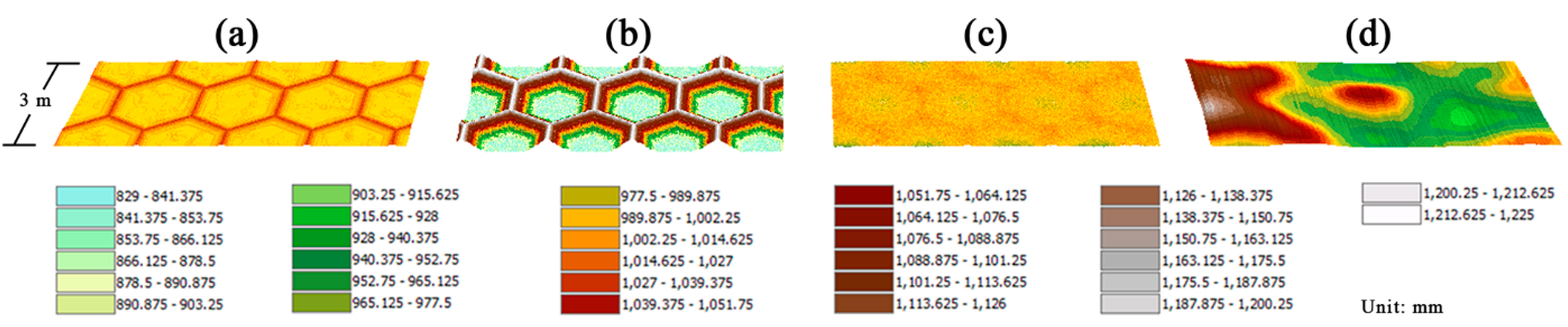
We generated four ideal DEMs (Figure 4) to simulate the four typical kinds of salt crust seen at Lop Nur. Computer graphics are used to create these DEMs, which are rendered as 3D models in ArcScene. Polygon ridges were designed as regular hexagons in an ideal situation, each pixel representing 1 cm in reality, with mm as the unit of height. The diameter of each hexagon was 200 pixels or 2 m in reality, referring to parameters measured in the field.

DEM a (Figure 4a) shows a salt crust in an early stage of evaporation crystallization, with polygonal cracks formed but uplifts are not very significant, approximately only 3 cm. The shape of these polygonal uplifts has been simplified to hexagons and some mixtures of sand and halite are expressed as tiny burrs in the central section of each unit, where it is almost flat. DEM b (Figure 4b) shows a stage where a well-developed honeycomb-shaped salt crust is developed, caused by underground saltwater. The height of this kind of salt crust in the field varies between 20 cm and 60 cm, while the uplifts in DEM b are wider and higher than those in DEM a, to a height of approximately 40 cm. The main difference between DEMs a and b is in the growth of the salt crust, as erosion is ignored. Growth of the early stage salt crust is the primary factor leading to the formation of a second-stage crust.

As discussed, while we generated DEMs a and b using computer graphics, DEM c (Figure 4c) was created from DEM b. Wind erosion was considered in this model because the level of underground brine would not have been high enough to support salt crust growth. Thus, we designed an iteration algorithm to simulate the processes of natural wind erosion in order to transform DEM b into c. The annual prevailing wind direction is NE in the Lop Nur playa [12], so that we can assume the wind is in a single direction without loss of generality. Because the algorithm is an iteration process, the results depend on the termination conditions and can be independent of wind velocity and duration. The major assumption of this algorithm is that the elevation of salt crust will change according to wind erosion in both the micro- and macro-scale. On the one hand, if any point on a surface is lower than the surrounding local, micro-scale areas (i.e., by several centimeters), when wind blows sand, there will be a higher probability that this point will accumulate sand. Similarly, if any point on a surface is higher than the surrounding local areas, there is a higher probability that it will be disintegrated by the wind. On the other hand, if any point is either lower than the average surface height across the global, macro-scale area (i.e., by several meters), then this point will be increased in height by the sand from wind, and vice versa. The further a given point is away from the average horizontal plane, the higher the probability will be.

We implemented this algorithm in a series of loops. Each loop traversed a DEM to decide whether a given pixel was depressed or a high point across a three-by-three neighbor domain by comparing it with all eight adjacent pixels. Thus, when a pixel is higher than a neighboring one, one point score is accrued, whereas when a pixel is lower than a neighboring one, a negative one point score is accrued. If a pixel score is positive, then height should subtract a random offset, or the pixel height should add this random offset. The reason why the random offset must be added to the height of a pixel when the score is zero is because there will be much more sand in the upwind direction. The random offset for micro-scale obeys normal distribution whose mean is 5 mm and the standard deviation is 1 mm. Here we assumed that the influence of wind was obeying the most common normal distribution and the parameters of the distribution were the empirical value.

In a global situation, when the height of a pixel is far from the average plane, an offset must be added that expresses the weight of this distance, as follows:

$${\mathrm{offset}}_{\mathrm{depression}}=0.1\ast {(\frac{avg-height}{avg-min})}^{0.5\ast noise},$$

(22)

and

$${\mathrm{offset}}_{upland}=-{\mathrm{offset}}_{\mathrm{depression}}.$$

(23)

In these expressions, avg, min, and max refer to the average, minimum, and maximum heights of a DEM, while noise is expressed as a random value obeying normal distribution whose mean is 5 mm and standard deviation is 1 mm. The parameters of the distribution were also the empirical value. Note that Equations (22) and (23) were based on a number of experimental tests.

The loop of this process terminates when the difference between the maximum and minimum is less than 8 cm, corresponding with field measurements. Results show that DEM c appears similar to real salt crusts that retain polygonal features, although this is not particularly clear.

Results show that DEM d (Figure 4d) comprises a Gaussian surface with an x-axis correlation length of 1.2 m, a y-axis correlation length of 0.8 m, and an RMS height of 8 cm. This DEM was generated using a surface algorithm [18], incorporating morphological parameters from field measurements [6].

To simulate an ideal situation, the two parameters discussed above (Materials and Methods) that comprise the four DEMs were taken into account, and the results are listed in

Table 1. Details of all sites.

Site Number	Longitude	Latitude	RMS Error in Length (mm)	Valid DEM Size		GLCM Score	Roughness
				x	y
LP-15-1	90.842229	40.356651	2.373	2990	198	0	1.25
LP-15-2	90.83774	40.353592	3.164	3020	227	1	1.33
LP-15-3	90.83382	40.3509	2.443	3015	219	0	1.36
LP-15-4	90.83095	40.348594	2.224	3093	275	0	1.3
LP-15-5	90.827736	40.346352	2.539	3112	213	1	1.3
LP-15-6	90.816787	40.338409	1.599	3102	208	1	1.47
LP-15-7	90.812159	40.334841	0.335	2975	246	1	1.36
LP-15-8	90.807275	40.3317	0.386	3001	177	2	1.35
LP-15-9	90.801751	40.327591	0.275	3026	273	3	1.27
LP-15-10	90.79745	40.324331	1.395	3151	199	2	1.49
LP-15-11	90.793049	40.321258	0.53	3042	211	3	1.36
LP-15-12	90.790395	40.319133	3.124	3044	178	2	1.6
LP-15-13	90.760539	40.297679	0.49	2967	278	3	1.7
LP-15-14	90.756461	40.294395	0.665	3020	284	4	1.5
LP-15-15	90.736102	40.279376	1.962	3033	297	3	1.89
LP-15-16	90.731691	40.276025	3.495	3026	273	3	1.7
LP-15-17	90.728515	40.27342	2.738	3128	283	3	1.78
LP-15-18	90.724791	40.269732	2.981	2943	299	2	1.91
LP-15-19	90.717863	40.264934	3.203	2688	310	3	2
LP-15-20	90.712889	40.260894	0.148	3206	273	3	1.74
LP-15-21	90.70947	40.258187	3.411	2591	236	4	1.88
LP-15-22	90.705714	40.255229	0.174	3039	301	4	1.84
LP-15-23	90.699589	40.250315	0.287	3139	242	4	2.07
LP-15-24	90.665578	40.234282	0.481	2868	297	4	1.69
LP-15-25	90.656112	40.23015	0.48	2894	222	3	1.5
LP-15-26	90.558418	40.191033	0.114	3020	128	3	1.45
LP-15-27	90.53351	40.180915	0.912	2454	140	2	1.39

. We then projected the four DEMs in two-dimensional space incorporating GLCM score on the x-axis and roughness on the y-axis, including data from other sample sites on the same graphic (Figure 5).

Characteristics of the salt crust evolutionary process are obvious (Figure 5). The tendency generalized by the green line in Figure 5 fits well with the rules outlined above; on the basis of point aggregation and information from sites, these regions can be manually classified into four categories. Of these, category A was not encountered in our research area, whereas the others are classified on the basis of similar ideal salt crust models, linked directly to ideal DEMs. Thus, if the rings identified from remote sensing images at Lop Nur do correspond to historical shorelines and the drying process has been steady, then the characteristics of salt crust should change according to the ideal model outlined above. Thus, based on the results of this cluster analysis as well as the geographic positions of sample points, we conjecture that sites LP-15-1 to LP-15-7 belong to category D. These sites nearest to the edge of the “big ear”, thought to be older salt crusts, are close to the ideal DEM d in our graphics, having low roughness and low GLCM scores. Sites LP-15-8 to LP-15-12 are all classified in model C2, which is a category defined as transition stage from C to B, although their indexes are a little different. These variations may partially explain the presence of bright and dark concentric rings on remote sensing images. Sites LP-15-13 to LP-15-20 except LP-15-14 and LP-15-18 belong to category C1, which means that salt crusts in this category are at middle evolutionary stages and erosion leads to the result. Sites LP-15-21 to LP-15-24 belong to category B, which is at a ridge-growing stage. It is notable that sites LP-15-25 to LP-15-27 are near the center of the concentric shoreline circles, whereas the characteristics of microrelief lead them to be similar with category C2. Among these sampling sites above, LP-15-14, LP-15-18, and LP-15-25 to LP-15-27 require further discussion.

The performance of SfM as an earth surface reconstruction technology has been evaluated against various alternative technologies such as traditional photogrammetry (e.g., [19]), total station and laser profilometer (e.g., [20]), as well as aerial (e.g., [21]) and terrestrial (e.g., [20,21,22]) LiDAR. SfM shows a relatively acceptable model accuracy in microtopography research. Different from methods used before, steel rulers as scale bars rather than ground control points (GCPs) are adopted as a model calibration reference in the reconstruction process. The models derived directly by PhotoScan without using control have a fine relative accuracy, but required scaling and geo-referencing. In this research focusing on the microrelief of salt crust, only the geometrical appearance and length are concerned. Deploying steel rulers throughout a scene is timesaving and economical as compared to assigning GCPs and measuring coordinates of GCPs by total station. The evaluation results of scale bars for all sites were less than 4 mm, which proves that the models are of high precision and reliable for intensive study. Another issue raised when reconstruction occurs without GCPs is that the trend surface of point cloud is not horizontal. This is resolved by multiplying the rotation matrixes to all points in the model.

Subsequently, two selective parameters were derived from the DEMs that were transformed from point clouds. Roughness is a scale-sensitive microtopography concept. For example, 0.5 m uplift is significant in a 3 × 3 square meter area but negligible in a 30 × 30 square meter one. To ensure that the roughness of all sites was compared in a same magnitude, the DEMs were uniformly clipped into 100 × 2400 pixels, which corresponds to 1 × 24 square meters in the real world. To statistically describe structured uplifts of salt crust, GLCM score was introduced to distinguish the intensity and consistency of uplifts in each site. If the uplifts were (1) low but in a good honeycomb shape, or (2) tall but in an irregular honeycomb shape, they were all estimated by the parameter as salt crust developing not so well. Situation 1 is suitable with the salt crust developing process hypothesis, but situation 2 presents the problem that the uplift will be underestimated. That is the reason why LP-15-18 is lower in GLCM score than its neighbor sites, although there are honeycomb-shaped ridges observed in the site (Figure 6). We infer that the salt crust may be influenced by an external force, such as a sudden inflow from upstream. The results of other sites reveal that these two parameters work well in quantifying salt crust microrelief at different stages.

Altitude difference between LP-15-1 and LP-15-27 is about 2 m, while the distance is about 30 km [23]. The slope of the Lop Nur lake basin, about 0.067‰, is so gentle that the shoreline is sensitive to weather change when the lake shrinks. For the classifications in Figure 5, it is assumed that the salt crust on the “big ear” develops without interruption and is exposed in the open air in chronological order. The area including LP-15-25, LP-15-26, and LP-15-27 dried out early, and was submerged before 1931 and then dried out again after around 1940 [23,24]. The developing process of salt crust here does not agree with the assumption we made above, and the microrelief turned out differently from what we predicted (Figure 7). While LP-15-14 and LP-15-18 show discriminative microrelief characteristics as compared to other neighbor sites, it is speculated that the shorelines where they are located are also interrupted by an inflow event, perhaps from the melting water from glaciers upon the Tianshan Mountains due to increasing temperatures.

4. Conclusions

Quantitative research about salt crust microrelief is important if we are to understand how this kind of landform evaluates over the long term. Because it is very hard to distinguish microrelief differences between sampling sites by eye, we used SfM and algorithms to extract microrelief features in order to quantify the salt crusts at Lop Nur. Thus, a series of precise digital 3D models constructed from close-range photos form the basis for this study. Measurements for microrelief roughness as well as the regularity of salt crust polygonal uplifts were used to distinguish the salt crusts, while GLCM scores were used to describe features of the latter. By applying these new approaches, we identified five key points which were representative of the drying shorelines at the time of crust formation, confirmed by comparison with neighboring sites in terms of values for numerical features. We speculate that sites LP-15-14 and LP-15-18 are shorelines that may be recovered by inflow from upstream.

Future field work incorporating approaches such as optical stimulated luminescence sampling will be carried out at the points identified in this study to determine drying periods and the reasons underlying the generation of salt crusts. These results will then be correlated to consensus data on paleoclimate, while additional data, including data from novel C-band synthetic aperture radar and images from unmanned aerial vehicles, will be used to further investigate these phenomena.