Article

Vertical Structure of the Water Column at the Virgin Islands Shelf Break and Trough

by
Giovanni Seijo-Ellis
1,*,
David Lindo-Atichati
1,2,3 and
Haydee Salmun
1,4
1
Earth and Environmental Sciences, The Graduate Center, The City University of New York, 365 5th Ave, New York, NY 10016, USA
2
College of Staten Island, Department of Engineering Sciences and Physics, The City University of New York, 2800 Victory Blvd, Staten Island, NY 10314, USA
3
Department of Earth and Planetary Sciences, American Museum of Natural History, New York, NY 10024, USA
4
Hunter College, Department of Geography, The City University of New York, 695 Park Ave, New York, NY 10065, USA
*
Author to whom correspondence should be addressed.
J. Mar. Sci. Eng. 2019, 7(3), 74; https://doi.org/10.3390/jmse7030074
Submission received: 22 February 2019 / Revised: 16 March 2019 / Accepted: 17 March 2019 / Published: 20 March 2019
(This article belongs to the Section Physical Oceanography)

Abstract

:
The steep US Virgin Islands Shelf Break (VISB) and the Virgin Islands Trough (VIT) at the Northeastern Caribbean Sea comprise a dynamic region of the Atlantic Ocean. In situ oceanographic data collected in the region during April 2017 were used to examine the spatial variability in temperature, density, salinity, and relative Chlorophyll-a. Analysis of data from the upper 300 m of the water column, that include deep and shallow water stations in the shelf break region, shows strong stratification of the water column. Stations shallower than 800 m along the shelf break are more variable in temperature, density, and salinity than those that are deeper than 800 m along the trough. For shallow stations, the mixed layer depth deepens along-shelf from West to East while at the deep stations the opposite occurs. Salinity maxima exhibit more variability in depth and range of values in the shallow stations compared to deep stations. Six different types of water masses that contribute to the strong stratification in the region were identified in our study: Caribbean Surface Water, Subtropical Underwater, Sargasso Sea Water, Tropical Atlantic Central Water, Antarctic Intermediate Water, and North Atlantic Deep Water. The upper level Caribbean Surface Water, Subtropical Underwater, and Sargasso Sea Water are present in shallow stations, indicating potential meridional intrusions from the VIT to the VISB which may not be resolved by current ocean circulation models and are not captured in satellite data. The analysis presented here indicates that competing physical processes may be controlling the vertical structure of the water column in the region and merit further examination.

1. Introduction

A long-standing challenge in ocean sciences, essential to assess and manage near-shore fisheries, is the understanding of the spatial structure and temporal variability of the coastal water masses. One of the key scientific challenges at the interface of coastal ocean dynamics and ecosystems pertains to quantifying the control exerted by shelf-slope exchange processes on the physical, chemical, and biological properties of continental shelves. For example, transport in the coastal ocean drives the exchange of larval fish populations and influences the population dynamics and genetic structure of marine species (White et al. [1] and Pineda et al. [2]). Driving mechanisms for shelf-slope exchange processes that influence biological activities can be external, such as processes driven by regional seasonal variation in the mean winds and distant river plumes moving into the area, or internal to the area of interest, such as those that generate fronts due to the interaction between local currents and tides with the changing bathymetry at the shelf break (see Palma et al. [3]). To investigate these processes we require high resolution measurements of physical properties such as temperature, salinity, density, as well as ocean circulation model outputs that describe the dynamics of coastal waters, all of which can potentially influence biological dynamics, see for example Baltazar-Soares et al. [4] and Smedile et al. [5].
Several studies have shown that the internal processes associated with the formation of shelf-break fronts in regions dominated by cyclonic flows (as well as anticyclonic ones) can generate shelf break upwelling of nutrient-rich waters to the surface (see Matano and Palma [6] and references therein). A study conducted by Linder et al. [7] showed that detachments of the bottom boundary layer in the Middle Atlantic Bight shelf break serves as a primary mechanism for pumping nutrient rich waters from the bottom towards the surface along isopycnal fronts and thus enhancing primary productivity within the frontal zone of the shelf break. Zhang and Gawarkiewicz [8] also showed enhanced biological productivity at shelf break fronts and how ocean circulation models can be employed to examine the seasonality of these mechanisms. In addition to these mechanisms, Rueda-Roa et al. [9] have shown that the seasonal strengthening of the wind curl serves as a primary mechanism for upwelling in the Southern Caribbean Sea.
The specific area of interest for the present study is the US Virgin Islands shelf break (VISB) between the islands of St. Thomas and St. Croix at the Eastern Caribbean Sea (Figure 1). The topography of that region is characterized by a relatively shallow (25 m) shelf that transitions into a highly steep gradient at its break towards the Virgin Islands Trough (VIT) (over 4000 m deep). Harlan et al. [10] showed that the surface flow around St. Croix is particularly complex. The constant easterly trade winds, mesoscale eddy activity, the Amazon and Orinoco river plumes, and the interactions between the shallow shelf and the deep VIT all combine to create a highly dynamic region of the Caribbean. A recent modeling study by Cherubin et al. [11] suggested that the timing of arrival and northward extent of the plumes from the Amazon and Orinoco rivers control the nature of the wake on both sides and ends of St. Croix. The angle of incidence of the incoming plume to St. Croix regulates the nature of the wake flow, resulting in a reversal from cyclonic to anticylonic flow with either attached or shed eddies. Such flow variability has the potential to control the manner in which offshore waters move onto the shelf break and beyond, therefore affecting the patterns of recruitment along the islands located between the islands of Vieques and Tortola. Additionally, Johns et al. [12] recorded the large 2009 Amazon River plume that intruded into the North Eastern Caribbean and noted that larval fish assemblages in the upper 100 m of the water column differed substantially from previous years’ observations. Furthermore, Quattrini et al. [13] showed that changes in water mass characteristics in the Northeastern Caribbean Sea result in species turnover at different depths associated with such water mass changes and conveys the importance exerted by water mass characteristics in controlling community structure in the region. The VISB is biologically unique because it includes two ecologically significant spawning aggregation areas 12 km South of St. Thomas: the Red Hind Conservation District and Grammanik Bank. Despite the importance of these Marine Protected Areas (MPAs), the exchanges of water masses between the VIT and these two spawning aggregation sites are to date poorly known [14].
The studies referenced above highlight the importance of using an integral approach that includes oceanic and biological dynamics in order to understand physical–biological interactions in the vicinity of shelf breaks. As a first step towards an integrated understanding of the physical ocean processes taking place at the VISB shelf front, the present analysis aims to describe, at a very fine spatial resolution, the spatial structure and variability of the water column at the VISB during April 2017, and to identify the water masses in the region. A description of the study area, data collection and methods is provided in Section 2. Results are described in Section 3 followed by a discussion in Section 4 and conclusions in Section 5.

2. Materials and Methods

In April 2017, we undertook a research expedition on board the National Oceanic and Atmospheric Administration (NOAA) Ship Nancy Foster and sampled the area of interest shown in Figure 1. A total of 106 in situ measurements made with Conductivity–Temperature–Depth (CTD) were taken within the region shown in Figure 1. For the present analysis, 35 CTD casts are used to examine data in the narrow region on each side of the shelf break to investigate exchanges between the VISB and the VIT. The CTD data were collected using a Sea-bird Scientific 9/11plus CTD system. The underwater unit (9plus) was installed on a rosette configured with a 24-bottle water sampler and instrumented with dual temperature, conductivity, and dissolved oxygen sensors. These Sea-bird sensors were factory calibrated just prior to the research cruise. The 9plus unit was also equipped with two WETLabs Environmental Characterization Optics fluorometers: one tuned to measure Chlorophyll-a (Chl-a) florescence, the second to measure Colored Dissolved Organic Matter fluorescence. Both fluorometers measure only raw voltages and served to provide relative concentrations. As such, we refer to the raw voltage data from the Chl-a fluorometer as relative Chl-a from here on. Following the cruise, the data set produced from the 9/11plus unit was post processed and quality controlled using a standard set of Sea-bird Scientific routines (“SBE Data Processing” suite, publicly available). Density profiles are calculated via the SBE Data processing suite from the measured temperature, conductivity and pressure.
The number for each station in Figure 1 corresponds to the sampling order during the campaign. Because our stations are a subset of a larger sampling cruise in the wider region, numbers missing in our stations list correspond to stations that are outside of our region of interest or to stations at which the CTD was deployed at the surface or in very shallow waters (15–30 m). Stations in the figure with more than two numbers correspond to the same geographical location where sampling took place twice at different dates. For example, Stations 29 and 30 where sampled to 300 m depth and 1 h apart. Stations 26 and 51 where sampled 2 days apart (04/17 and 04/19) at approximately the same time of day, 10:00 p.m. The time interval between stations depends primarily on the travel time between stations and the depth at which the CTD cast was completed in each station. The depth of the CTD cast in turn is dependent on the water depth at each station. We focused our analysis on profiles of temperature, density, salinity, and relative Chlorophyl-a, and classify data stations according to their water depth. The 800 m isobath in Figure 1b approximately delineates the center of the shelf break gradient and was used as the depth limit for the classification. Stations located in water depth <800 m are classified as shallow stations and those in water depth ≥800 m are classified as deep stations. Figure 1 shows station distribution and classification; shallow water stations are identified with black circles, and deep water stations with magenta circles. Additionally, the stations enclosed by the white box in Figure 1, with the exception of Station 42, were used to examine variations of the water column in the cross-shelf direction; this group is referred to as the North–South transect and includes both shallow and deep stations. The resulting groups (shallow, deep, and North–South transect) with their respective stations are shown in Table 1. For the North–South transect, we have chosen to exclude Stations 29 and 42, because they are sampled twice, and the remaining stations (82 through 86) are sampled consecutively one after the other, limiting time differences.
We first present illustrative profiles of the region to provide an overall description of the variability observed in the region. These profiles are examined for characteristic along and cross-shelf differences of all profiles. We follow with an examination of variations in the cross-shelf direction to observe changes along the North–South transect stations, from the VIT to the VISB. We then examine all profiles from shallow stations, color-coded according to their longitude, to inspect patterns and differences in the along-shelf direction. This examination is performed for the deep water stations as well. In addition, we compare variability between shallow and deep stations by examining the standard deviations of temperature, density, and salinity at each depth level for each group. We also calculated the ranges of temperature, density, and salinity at different depth intervals for both shallow and deep stations as further test of variability between the two groups. For the North–South transect, we examine the difference of each profile from the mean profile of the group. Finally, Temperature–Salinity (TS) diagrams to identify water mass types in the region are presented.
We note that shallow stations, as well as several deep stations, have CTD casts that only reach down to the first 300 m of the water column. Below that depth, differences among profiles from different stations were negligible and no variability with depth was observed in water characteristics. Consequently, and for the sake of uniformity, we limited the analysis to the first 300 m of the water column, except when drawing the TS diagrams.

3. Results

3.1. Defining Features of the Water Column

In order to highlight the variations among profiles, we selected the three shallow stations (Stations 60, 48, and 22; black line) and the three deep stations (Stations 61, 50, and 23; magenta line) shown in Figure 2. The data in Figure 2 show that a well defined mixed layer is representative of the waters in the region. Variations exist among profiles and this variability appears to characterize the water stratification in the region, irrespective of depth of water. Here, we define the depth of the mixed layer as the depth at which density changes by 0.1 kg/m3 or more of its surface value. The value is within the range of 0.01–0.125 kg/m3 used in several previous studies, see [15,16,17]. Figure 2 shows that the differences in the depth of the mixed layer of shallow stations as compared to deep stations are more pronounced than the differences within shallow and deep stations themselves. For example, using the density data of Figure 2b, the maximum difference between the depth of the mixed layer at Station 23 and that at Station 22 is 48 m. Stations 50 and 61, both deep, have a mixed layer depth difference of 10 m and stations 60 and 22, both shallow, have a mixed layer depth difference of 25 m. The temperature, density, and salinity of the mixed layer varies among profiles, although the variability in temperature is much less than that in density and salinity. For example, there is a 0.3 kg/m3 difference (12% of the density range) in the density of the mixed layer between Stations 60 and 48 (both shallow), a difference in the salinity of 0.25 Practical Salinity Units (PSU) (24.5% of the salinity range), while the difference of the temperature of the mixed layer is about 1/8 of a degree Celcius (1.25% of temperature range). Figure 2, in particular Figure 2a,b, also shows a prominent feature of the profiles as a marked step observed where the mixed layer transitions into the pycnocline followed by staircase-like variations in depth. Finally, Figure 2c shows that below the mixed layer, the salinity profiles are characterized by a belly-like shape with a salinity maximum ranging from approximately 120–140 m in depth.
We select representative pairs of profiles from Figure 2 to examine in detail the water structure between the shallow shelf and the deep trough. These representative pairs are Stations 60 and 61, Stations 48 and 50, and Stations 22 and 23 (as identified in Figure 1). We examine the differences in temperature and density within each pair and how these differences evolve in the along-shelf direction (West to East). Using the data in Figure 2a,b, we observe that for the shallow stations the mixed layer depth ranges from 40 m (Station 60) to 70 m (Station 22). This indicates a deepening of the mixed layer on the shallow part of the shelf as we move from West to East. For the deep stations, the mixed layer depth ranges from nearly 60 m (Station 61, West section of study area) to approximately 28 m (Station 23, East section of study area). Hence, in contrast with the observations at the shallow stations, the mixed layer for the deep stations becomes shallower from West to East. The data also show that the difference in the depth of the mixed layer between the stations in each pair increases from 20 m (Stations 60 and 61) to 45 m (Stations 22 and 23), as we move from West to East.
The salinity profiles of Figure 2c show that the salinity maximum occurs over the depth range of 115–145 m. At the deep stations, Stations 61, 50, and 23 (from West to East), the salinity maximum occurs within a difference range of 3 m, at an average depth of 138.4 m. For the shallow stations from West to East, the salinity maximum at Station 60 occurs at 133 m, at Station 48 occurs at 116 m, and at Station 22 the salinity maximum occurs at 120.7 m.
These values, summarized in Figure 3, indicate a variability in the depth of the salinity maximum not observed in the along-shelf direction in the deep stations. In addition, we note that the difference between shallow and deep stations to the West (Stations 60 and 61) is much lesser than the difference between shallow and deep stations as we move East.
It should be noted that the CTD casts pairs presented in this section were carried out within 3 consecutive days, each pair at approximately the same time of day. Casts for the pair made of Station 60 (shallow) and Station 61 (deep) were conducted 1.5 h apart. The same applies to the pairs made of Stations 48 and 50, and Stations 22 and 23. Although we strove to minimize time intervals between CTD casts, we recognize that these differences in times at which measurements where taken might result in a small contribution to the observed differences described above. These contributions were tested by calculating the differences between profiles measured during different days but at the same time of day ±3 h. The contributions to observed differences due to sampling time intervals are smaller than those due to spatial differences.

3.2. Comparison of Cross- and Along-Shelf Groups

In this section we focus on examining all data from stations grouped into the three categories previously described, shallow stations, deep stations, and North–South transect, shown in Figure 1. Our purpose here is to examine variability of water properties in the cross-shelf direction and in the along-shelf direction. For the cross-shelf direction we use the stations grouped in the North–South transect, which includes both shallow and deep stations.
Figure 4 shows the profiles of temperature, density, salinity and relative Chl-a for North–South stations, color-coded according to latitude as shown in the sidebar of the figure.
The figure shows that variations exist among profiles and that such differences characterize the water stratification in the region, irrespective of depth of water. The profiles in Figure 4b show that northernmost shallow stations (red) have a deeper mixed layer, reaching 70 m, than the southernmost and deep stations (white and blue profiles). Figure 4b,c show that southernmost stations (blue profiles corresponding to Stations 85 and 86) have fresher surface water of both low density and salinity down to 30 m depth. The mixed layer of these stations, 86 and 86, is shallower (around 30 m) than that of the northernmost profiles (near 60 m). Below the mixed layer of Stations 85 and 86, there is a steep salinity and density gradient indicative of strong stratification from 30 to 40 m depth. Below the strong gradient for both stations, Figure 4b,c, there is a near-homogeneous layer between 45 and 60 m with similar properties as the other stations. The steep gradient in Stations 85 and 86 could be characterized as a temporary halocline, that could result, for example, from riverine/land outflows and/or rain. The National Weather Service [18] reported a total of 172.72 mm of observed rain total during April 2017 for St. Croix, approximately 7 km south of Station 86, making a rain event a likely contributor to the strong stratification observed in the first 70 m in Figure 4b,c.
Figure 4d shows relative Chl-a concentration profiles, Chl-a is a proxy for biological productivity and is associated, among others, with river plumes. The profiles show relative concentrations in the 0.06 to 0.1 range. The profile distribution shows that relative Chl-a concentrations slightly increase towards the northernmost stations, which is also the shallowest (Station 82). The profile for Station 82 in Figure 4d also shows variability between 50 and 130 m, that is potentially associated with higher productivity over the shelf.
We calculated the mean profiles of temperature, density, and salinity for the stations in the North–South transect and calculated the difference of each profile from the mean. The differences where plotted in depth with the color representing the latitude of the station. Figure 5 shows the differences for density and salinity, temperature does not show any discernible patterns or additional information and is not shown. The differences in density (Figure 5a), and salinity (Figure 5b) show an almost identical pattern for the first 120 m of water depth, approximately. Such pattern is indicative of salinity driven density in this part of the water column. Below 120 m, the pattern becomes less discernible, indicating that density is now contributed to by both temperature and salinity. The negative differences in salinity in the 0–30 m depth range correspond to salinity values that are lower than mean values and the same observation holds for values of density, as shown in Figure 4. Lower salinity values near the surface can be the result of rain events, which in this area will affect water salinity but have very little effect on water temperature ([19]).
The profiles for all shallow water stations are shown in Figure 6, but their colors represent the longitude of the station as shown in the sidebar. Figure 6b shows differences in the mixed layer depth ranging from 40 m to 80 m, approximately. Below the mixed layer, the profiles in Figure 6 exhibit a wider spread in values, an indicator of increased variability among temperature, density, and salinity profiles. The increased variability is associated with the corresponding cline of temperature, density, and salinity.
Both, density and salinity, show similar distributions in the mixed layer values. Easternmost stations (red) have saltier and denser water than stations towards the West (blue), and that pattern is specially notable at the surface (red and blue profiles, Figure 6b,c). This suggests that differences in the mixed layer density are contributed to by salinity differences as shown in Figure 6c. The relative Chl-a profiles in shallow stations show a slight increase in relative Chl-a maxima as compared to the deep stations in the North–South transect. The shallow stations towards the center of the group (white and light red colors in Figure 6d) exhibit greater relative Chl-a maxima than the stations at either end of the group, an indicator of higher productivity between 100 and 120 m for the center stations.
Figure 7 shows temperature, density, salinity, and Chl-a for the deep water stations, color-coded by their longitude. The depth of the mixed layer for the deep stations ranges from 20 m (easternmost, Station 23) to 60 m (center and western stations). The variation of the mixed layer depth indicates a deepening of the mixed layer in the along-shelf direction from East to West as described in the previous subsection.
Similar to the westernmost shallow stations, the westernmost deep stations show lower salinity and density along the mixed layer, Figure 7b,c while the observable differences in temperature in this layer are comparatively small. This is another indication of the larger contribution of salinity to the density along the mixed layer and transition into the pycnocline. In contrast to the shallow stations shown in Figure 6, the spread of the profiles in Figure 7 indicates less variability between profiles. The relative Chl-a concentrations shown in Figure 7d are within the same range as the shallow stations, but the relative concentration maxima for deep stations have lower values. Furthermore, the largest maxima for the deep stations occur at the stations on both ends of the group (blue and red profiles) and not at the center as for the shallow stations.
We calculated the mean profiles of temperature, density, and salinity for the shallow stations, and proceeded similarly for the deep stations. The means, in our case, provide a metric to compare differences in the temperature, density, and salinity between shallow and deep stations. We then calculated the standard deviations from the mean temperature, density, and salinity at each depth level for shallow, and deep stations. The standard deviations from the mean profile of each group are plotted at each depth using error bars on top of the corresponding mean profiles, Figure 8. For visualization purposes, we have plotted the standard deviation error bars every 5 measurements. The standard deviations, in our case, provide a metric of how much profiles vary from their mean among shallow stations, and among deep stations.
Figure 8 shows that for the top 20–30 m, the standard deviations are similar for both shallow and deep stations. In the transition from the mixed layer depth into the pycnocline the standard deviations for shallow stations start increasing progressively. For the deep stations, the transition from the mixed layer into the pycnocline is characterized by a slight increase then decrease in standard deviations, Figure 8b. Figure 8 shows that below the mixed layer, the standard deviations for shallow stations are greater than the standard deviations for deep stations. These greater standard deviations are indicative of more variability among the shallow stations than the deep stations. Finally, the standard deviations after approximately 200 m start decreasing, indicating that below 300 m variability decreases and profiles become uniform in depth, Figure 8b.
We have also calculated the average range of temperature, density, and salinity for shallow and deep stations for the following depth intervals: 0–50 m, 51–100 m, 101–200 m, and 201–300 m. The calculated ranges are shown in Table 2. With the exception of the ranges of temperature, density, and salinity for 0–50 m depths, the ranges for shallow stations are greater than the ranges for deep stations. The greater ranges for shallow stations are further indication of more variability among the shallow group profiles as compared to the deep group profiles.

3.3. Water Mass Identification

The commonly accepted vertical stratification in the region is represented in the Virgin Islands Shelf Break and Trough as staircase-like features, as seen in the upper 300 m of the water column in our data and described in our analysis. Vertical stratification can be caused by different mechanisms including the intrusion of water masses of distinct origins at different depths. Quattrini et al. [13] identified the water masses in the region and their defining characteristics based on temperature and salinity data and following the water mass characteristics presented by [20,21,22,23,24,25,26]. The Temperature–Salinity (TS) diagrams they present specifically reveal the types of water masses reaching the region. These types of water masses are: Caribbean Surface Water (CSW), Subtropical Underwater (SUW), Sargasso Sea Water (SSW), Tropical Atlantic Central Water (TACW), Antarctic Intermediate Water (AAIW), and North Atlantic Deep Water (NADW). The existence of these different water masses in the region is an indicator of externally sourced contributions to local water column stratification in the VIT that can also affect stratification over the shelf. Using the temperature, salinity, and oxygen data from all sampled stations, we produced Temperature–Salinity diagrams shown in Figure 9. We employed the approximate ranges of depth, temperature and salinity presented by [13] to identify the water masses in our data. These water masses contribute to the unique features of the vertical structure of the water column at the VISB and VIT.
Figure 9a shows that CSW with low salinity dominates the upper part, and is followed vertically by SUW. In the Subtropics, where evaporation exceeds precipitation, surface water becomes more saline and sinks to a neutral buoyancy level forming SUW. Further down, salinity starts decreasing as the column transitions from SUW to SSW. The transitions from low surface salinity (CSW) into a salinity maximum (SUW) back to lower salinity (SSW) causes the characteristic belly-like shape in the salinity profiles of the region which we have noted before (Figure 4c, Figure 6c, and Figure 7c). SSW is followed by a low oxygen TACW mass after which a salinity minimum is reached between 700–1000 m (Figure 9b where a water mass of AAIW is found. A deep salinity maximum characteristic of upper NADW follows AAIW. The water masses shown in our data are in good agreement with those presented by Quattrini et al. [13]. The approximate ranges of the water mass characteristics are provided in Table 3. In addition to the depth, temperature and salinity ranges obtained from [13] to identify the water masses, we have provided the approximate range of oxygen and the approximate density interfaces of the water masses that serve to further characterize them.
Figure 9b shows the TS diagrams with depth. This TS diagram shows that CSW, SUW, and SSW are present at stations located in water depth <300 m. This presence may indicate that intrusion of waters take place between the VIT and VISB, likely redefining the structure of the water column in the shallow region. The diagram also confirms the presence of strong stratification in the upper 300 m as observed in the previous sections. Below 300 m, the TS curves run more parallel to the isopycnals, indicating weaker stratification.

4. Discussion

We began the analysis presented here by looking at defining features and general structure of different profiles. Variability is characterized by differences in the mixed layer depth as well as staircase style profiles (Figure 2). The vertical variability causing the staircase style profiles is an indication of strong stratification of the water column. The TS diagrams from all stations confirm vigorous stratification in the upper 300 m of the water column.
A close inspection of characteristic profiles, shallow (<800 m depth) and deep (>800 m depth), shows more variability in the mixed layer depth and salinity maxima among shallow stations as compared to deep stations. Remarkably, we showed that the mixed layer deepens in the along-shelf direction towards the East among shallow stations while in deep stations the mixed layer deepens towards the West. Although attributing these changes to specific mechanisms is out of the scope of this study, a simple hypothesis is that there is a difference in wind stress in the VISB as compared to the VIT. An alternate hypothesis is that there is a difference in water flow regimes over the VISB compared to the VIT. Preliminary analysis of hull-mounted Acoustic Doppler Current Profiler data (not shown) indicates that the flow across the VIT during sampling was predominantly from East to West, in agreement with the prevailing flow of the region, and relatively uniform in its direction along the first 100 m of depth. Near the shelf break though, this flow uniformity is lost, possibly due to interactions with the fast changing bathymetry, and this interaction may contribute to the along-shelf variations of the mixed layer and characteristics of the water column between shallow and deep stations. Additionally, based on the discussions presented by Chapman and Lentz [28], Matano and Palma [6] and references therein, the interaction between the flow and the bathymetry merits further examination. Such examination would be essential to assess physical–biological interactions in the region.
Examining the North–South transect, the deeper stations in the group have a shallower mixed layer (15 m to 35 m deep as compared to 75 m) and fresher surface water than the shallower stations in the group, Figure 4b,c. Such differences may be due to rain events in the vicinity of the deeper stations, and is supported by rain data collected in the island of St. Croix (7 km south of Station 86) during April 2017. Below the mixed layer, differences in salinity and density become negligible and the vertical profiles uniform. The effect of rainfall on temperature profiles is minimal since in these regions raindrop temperatures are not significantly different from environmental temperatures ([19]).
Although relative Chl-a concentrations remained low during the sampling period, deeper stations have slightly lower concentrations than shallower stations (Figure 4d, Figure 6d, and Figure 7d). The ranges of CTD-obtained relative Chl-a concentrations were validated against satellite derived data using the Goddard Earth Sciences Data and Information Services Center GIOVANNI tool [29]. The data covers the period from 30th March to 9th May 2017, which coincides with the period of cruise sampling. The satellite derived Chl-a concentration data is in the range of 0.0 to 0.16 mg/m3, which represents one order of magnitude less than the Chl-a concentrations in the previously mentioned 2009 Amazon River plume discussed by Johns et al. [12]. Similarly to what our in situ data indicated, the satellite image in Figure 10 also reveals low Chl-a concentrations in the region of the deeper stations and increasing concentrations towards the region of shallower stations. This pattern is clearly illustrated in the area of the satellite-derived Chl-a map where the shelf break is closely outlined by a steep Chl-a gradient: Chl-a concentration reaches a minimum of 0.06 mg/m in the far field between St. Croix and St. Thomas; increases from 0.06 mg/m to 0.11 mg/m from the far field to the 250 m isobath; increases from 0.11 mg/m in the 250 m isobath to 0.16 mg/m in the 40 m isobath; and remains at 0.16 mg/m in shallow waters in between 30 m and 40 m. Noteworthy, a portion of the shelf waters can be considered optically shallow (<30 m) and are potentially affected by the bottom albedo effect causing overestimates of Chl-a over these waters. Nevertheless, there is still a high Chl-a gradient which starts away from the shelf at a depth of 250–300 m. Considering the location of the 30 m isobath respect to the extent and location of the gradient of Chl-a, Figure 10 still indicates increased Chl-a concentrations towards the shelf. Therefore, our relative Chl-a data, and that shown in Figure 10, are indicative of productivity over the shelf one order of magnitude higher compared to the trough.
Regarding variability between shallow and deep stations, the deep stations show certain uniformity that the shallow stations lack. This is shown by the wider spread in profiles, compare Figure 6a and Figure 7a for example, and supported by the standard deviations shown in Figure 8. In general, the standard deviations of shallow stations are greater than the standard deviations of the deep stations and thus indicate larger variability. Near 200 m, the standard deviations for both shallow and deep stations, start decreasing. The decrease in standard deviations indicates that variability decreases with depth. This was an important feature for deciding to evaluate just the upper 300 m of the water column (see Section 2). In addition, we examined the ranges of temperature, density, and salinity at different depth intervals and found that below 50 m depth, shallow stations exhibited larger ranges than the deep stations. The difference in ranges of the temperature, density, and salinity profiles provide further evidence that the shallow stations exhibit more variability than the deep stations. We hypothesize that one of the reasons for the differences in the vertical structure between shallow and deep stations is that the shallow stations provide more efficient and faster vertical mixing which allows for quicker adjustment of the water column. Therefore, the features of the water column can vary faster among shallow stations as compared to deep stations. The differences and variability between shallow and deep stations can also be contributed to by other mechanisms such as those discussed in the introduction, including but not limited to, internal waves and/or wind forcing [3,9].
We finalized our analysis by looking at T-S diagrams that include data from all stations. With the water mass characteristics compiled by Quattrini et al. [13], we were able to identify 6 water masses in the region: CSW, SUW, SSW, TACW, AAIW, and NADW. The presence of these masses is an indicator of external contributions to the strong local stratification in the region. The TS diagram in Figure 9b shows that the shallow VISB is dominated by CSW, SUW, and SSW, implying possible intrusions of waters from the VIT to the VISB that can take place for at least the top 300 m of the water column.
Corredor and Morell [20] show that Caribbean Surface Water to the South of Puerto Rico exhibits variability throughout the year mainly influenced by riverine outflows. Nevertheless, our region is not affected by significant riverine outflows from the surrounding islands, and the dominant East to West flow would transport any riverine outflows from Puerto Rico away from our region (the exception being the occasional intrusions of Amazon/Orinoco river plumes). Additionally, the temperature and salinity data presented by Quattrini et al. [13] was taken during October 2013 and shows the same range of data values as our April 2017 data set. These findings suggest that variations of the vertical structure of the water column below the Caribbean Surface Water mass may not be significant throughout the year, and the spatial pattern we present here are consistent year long. Thus, the larger variability over shallow stations as compared to deep stations, and the strong stratification observed in our data are likely representative of the general structure of the water column throughout the year. The occurrence of occasional phenomena such as Amazon/Orinoco river plumes and storms would force additional variability that can redefine the vertical structure for a short period of time. An extensive sampling project in combination with satellite remote sensing would provide the appropriate information to look at variations in the near-surface water structure at seasonal to year time-scales.
Johns et al. [30] discuss a potential seasonal component to the total Atlantic inflow into the Caribbean that could serve as an additional driver of variability and stratification in the region. The high resolution sampling we have presented, captures the inflow of Atlantic waters into the Caribbean and the strong variability in the vertical structure of the water column in the shelf and trough of the Virgin Islands. Quattrini et al. [13] showed that the presence of these water masses results in distinct vertical variation of fish communities in the Northeastern Caribbean Sea. How such potential seasonal cycle of the total inflow affects the strong stratification that drives distinct vertical variation of fish communities remains to be understood. How internal and external mechanisms for shelf-slope exchange processes that influence biological productivity, such as those discussed by [3,6,7,9,10,11,12,20,28,30] can be applied to the region, and potentially drive physical–biological interactions, merits further examination. Here we have presented a first high resolution examination of physical properties measurements in the region that are necessary to examine such processes.

5. Conclusions

The analysis we present here describes the vertical structure and identifies the water masses present at the VISB and VIT. Our work provides further evidence supporting several previous works addressing physical dynamics in the region. These physical dynamics may have biological implications for the region. Here we offer the very first step to examine possible local and external physical mechanisms at the shelf break and shed light to better understand the physical–biological interactions in the region. Our main conclusions are:
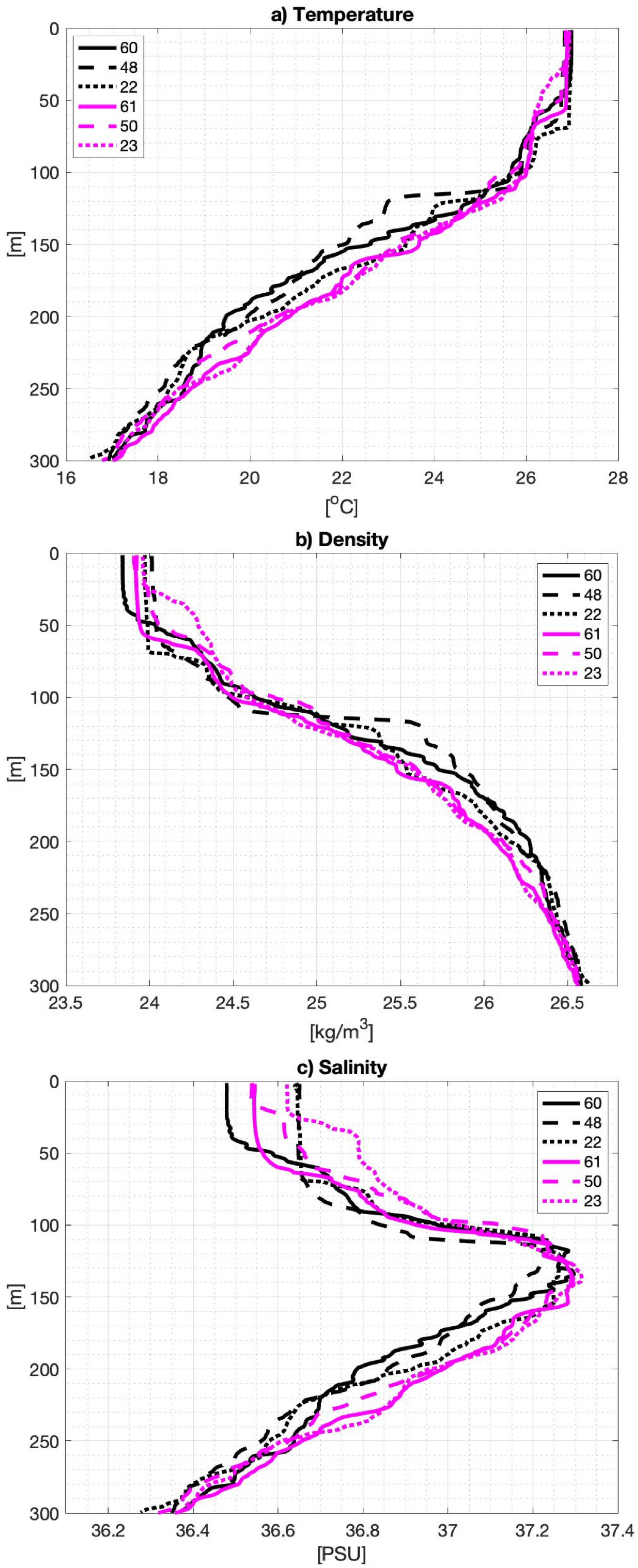
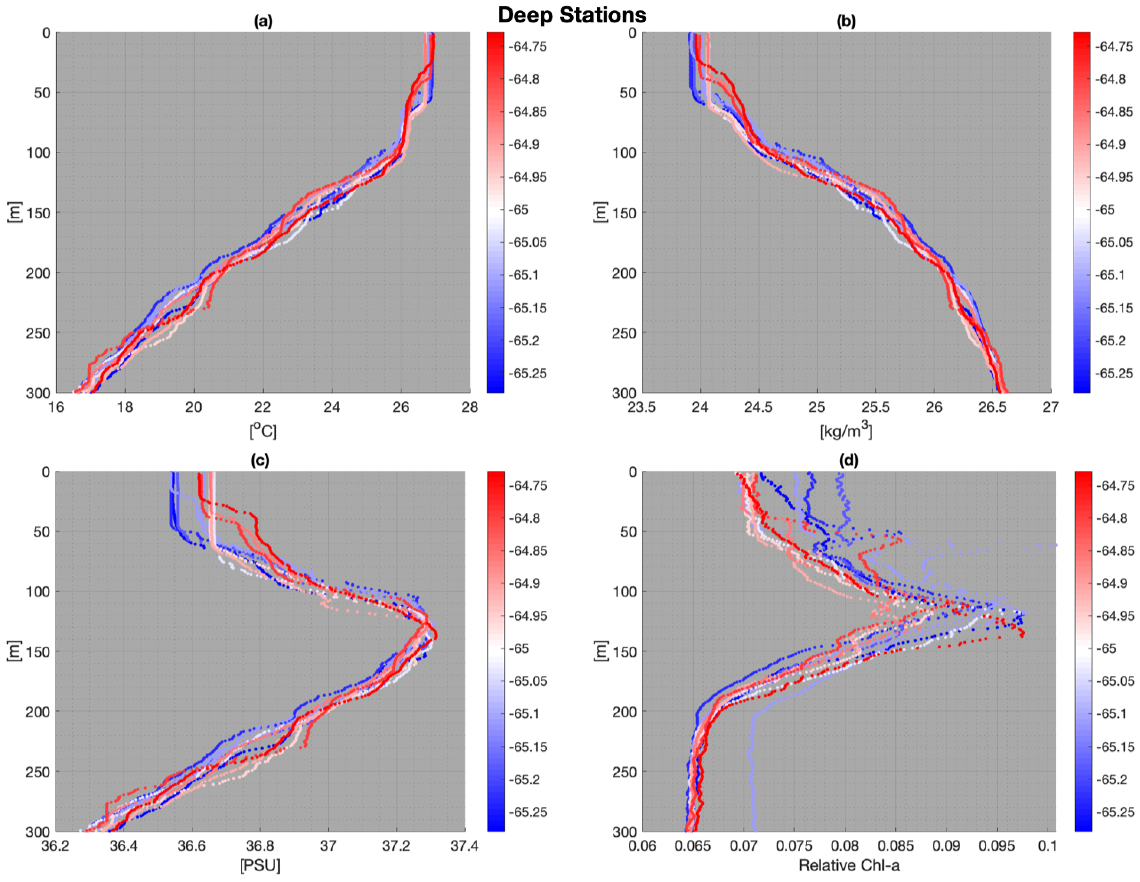
  • Differences exist in temperature, density, and salinity of the mixed layer among stations within the same group. For shallow stations the depth of the mixed layer is more variable and becomes shallower to the East. The opposite occurs for the deep stations.
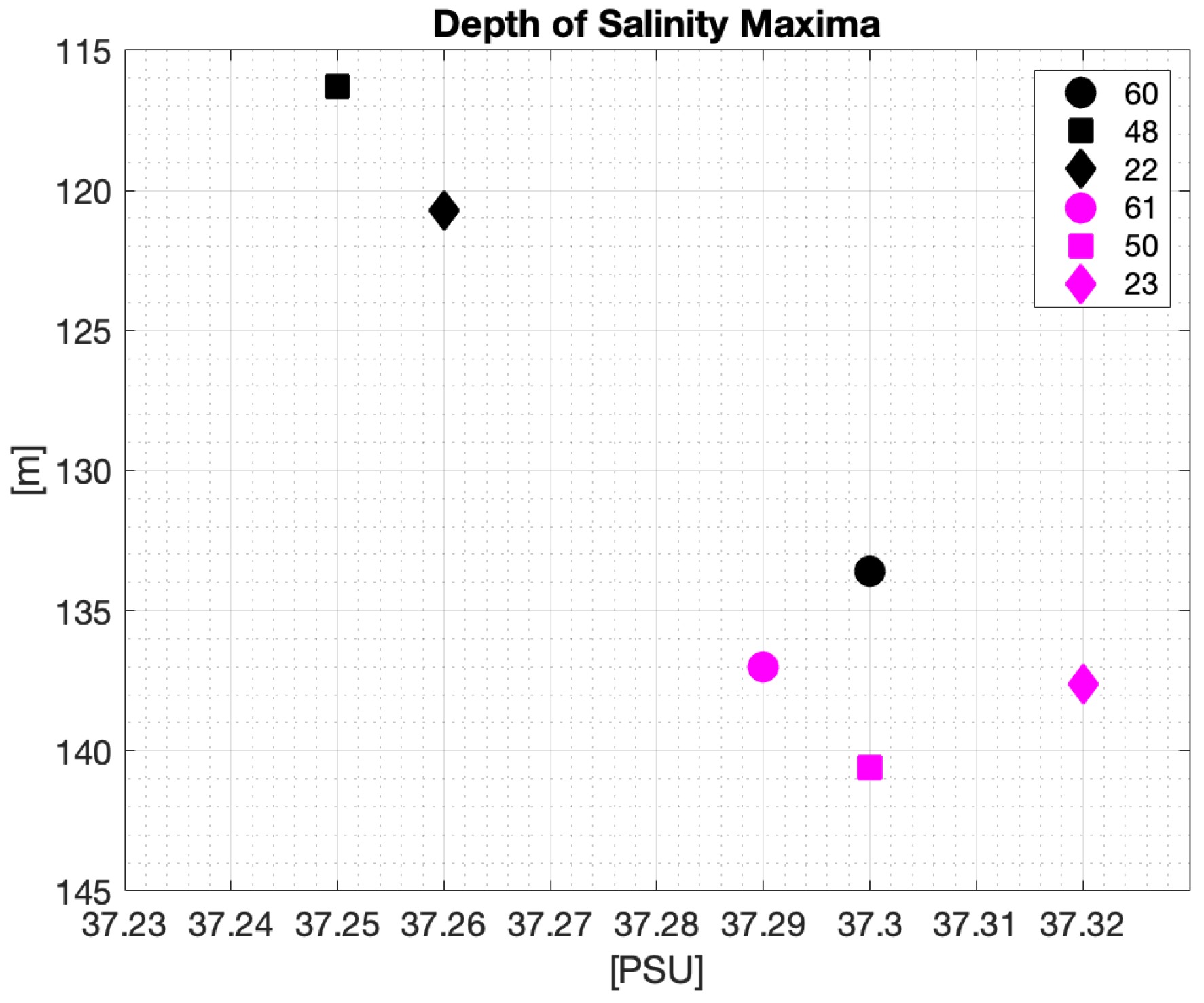
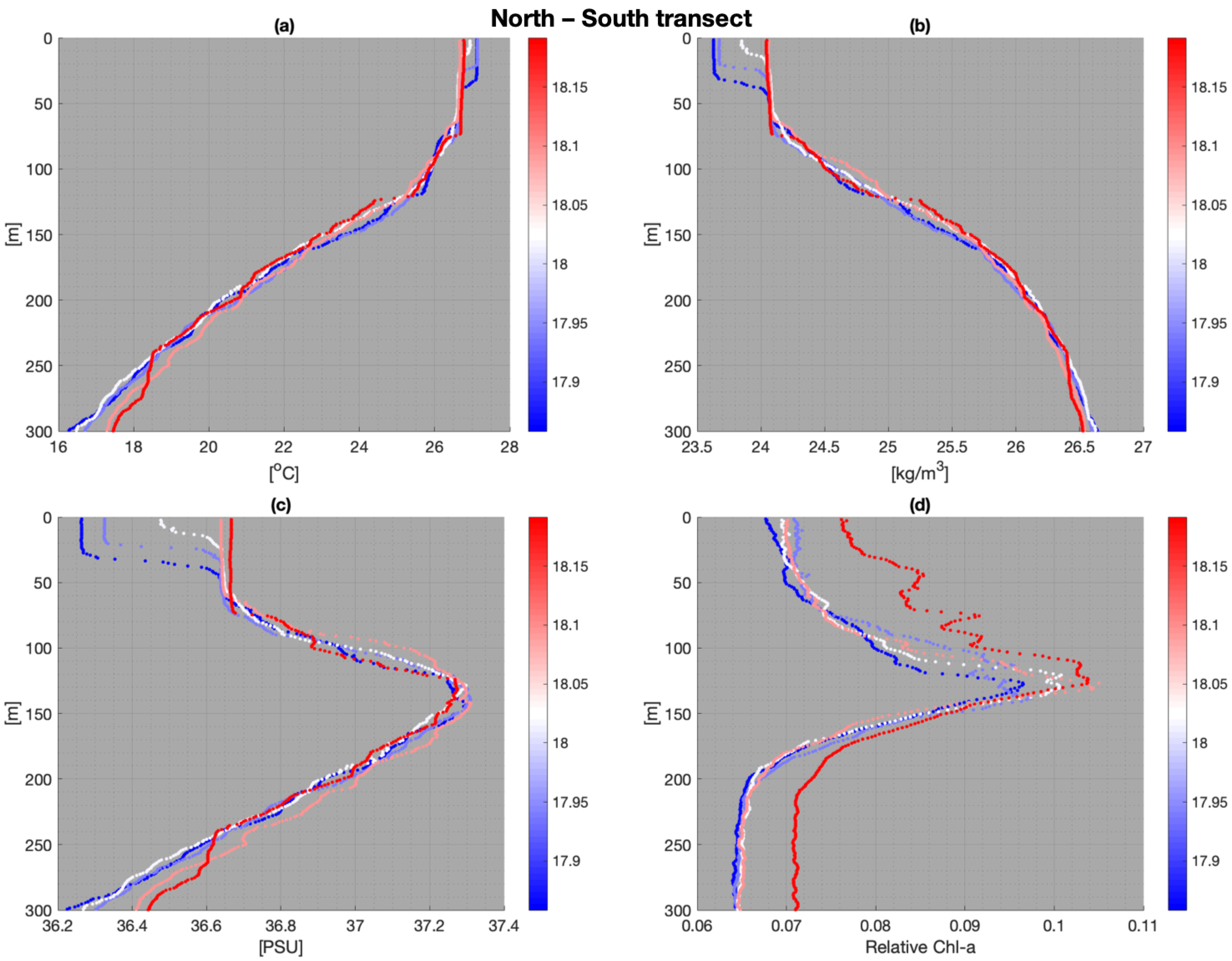
  • The transition between the mixed layer and the pycnocline in both shallow and deep stations is characterized by a marked step followed by staircase-like profiles, indicating strong stratification of the water column.
  • Variations in temperature, density, salinity, and chlorophyll-a exist among shallow and deep stations but variability is higher in shallow stations as shown by comparing standard deviations between shallow and deep stations.
  • The strong vertical stratification that characterizes the vertical structure of the water column in the region is a result, in part, of six water mass types present in the Northeastern Caribbean sea: Caribbean Surface Water, Subtropical Underwater, Sargasso Sea Water, Tropical Atlantic Central Water, Antarctic Intermediate Water, and North Atlantic Deep Water.
  • CSW, SUW, and SSW water mass types dominate the first 500 m of the water, which indicates that intrusions of these water masses onto the VISB may potentially occur.
The present work lays solid foundations to enable future companion sampling surveys, a connectivity study, and a modeling effort. A companion future cruise would increase the timeline and groundtruthing of our description. The framework presented here would be expanded to examine surface connectivity by using ocean drifter data and satellite remote sensing to further understand the dynamics between the VISB and VIT. A broader description of observations in the region will then be employed in hand with an ocean model to propose specific mechanisms for the observed water structure characteristics, and to explore physical–biological interactions.

Author Contributions

G.S.E., D.L.A. and H.S.: conceptualization and methodology; G.S.E., D.L.A: data collection plan; G.S.E.: data collection and processing; G.S.E., D.L.A., H.S.: data analysis; G.S.E.: original draft preparation; G.S.E., D.L.A and H.S.: review and editing.

Funding

Partial support for G.S.E. was provided by a CUNY Science Fellowship. This research was partially funded by the PSC-CUNY Research Foundation Award 61687-00 49 to H.S. and D.L.A. The APC was also funded by PSC-CUNY Research Foundation Award 61687-00 49.

Acknowledgments

Data presented in this paper were collected during NF-17-03, a Coral Reef Ecosystem Research (CRER) cruise conducted aboard the NOAA Ship Nancy Foster in 2017. CRER is supported by NOAA’s Atlantic Oceanographic and Meteorological Laboratory (AOML) and Southeast Fisheries Science Center (SEFSC) in Miami, Florida. We thank the CRER project for providing the data used for analysis in this paper. Additional thanks to Ryan H. Smith of AOML for recommendations towards improvement of the manuscript. Special thanks to Barbara Muhling of UC Santa Cruz for additional insights into the analysis. Data are available upon request by contacting: [email protected] at NOAA/AOML in Miami, FL.

Conflicts of Interest

The authors declare no conflict of interest. The founding sponsors had no role in the design of the study; in the collection, analyses, or interpretation of data; in the writing of the manuscript, and in the decision to publish the results.

References

  1. White, C.; Selkoe, K.A.; Watson, J.; Siegel, D.A.; Zacherl, D.C.; Toonen, R.J. Ocean currents help explain population genetic structure. Proc. R. Soc. B 2010, 277, 1685–1694. [Google Scholar] [CrossRef] [Green Version]
  2. Pineda, J.; Hare, J.A.; Sponaugle, S. Larval Transport and Dispersal in the Coastal Ocean and Consequences for Population Connectivity. Oceanography 2007, 20, 22–39. [Google Scholar] [CrossRef] [Green Version]
  3. Palma, E.D.; Matano, R.P.; Piola, A.R. A numerical study of the Southwestern Atlantic Shelf circulation: Stratified ocean response to local and offshore forcing. J. Geophys. Res. Oceans 2008, 113. [Google Scholar] [CrossRef] [Green Version]
  4. Baltazar-Soares, M.; Biastoch, A.; Harrod, C.; Hanel, R.; Marohn, L.; Prigge, E.; Evans, D.; Bodles, K.; Behrens, E.; Böning, C.; et al. Recruitment Collapse and Population Structure of the European Eel Shaped by Local Ocean Current Dynamics. Curr. Biol. 2014, 24, 104–108. [Google Scholar] [CrossRef] [PubMed] [Green Version]
  5. Smedile, F.; Scarfi, S.; De Domenico, E.; Garel, M.; Glanville, H.; Gentile, G.; Cono, V.L.; Tamburini, C.; Giuliano, L.; Yakimov, M. Variations in Microbial Community Structure through the Stratified Water Column in the Tyrrhenian Sea (Central Mediterranean). J. Mar. Sci. Eng. 2015, 3, 845–865. [Google Scholar] [CrossRef] [Green Version]
  6. Matano, R.P.; Palma, E.D. On the Upwelling of Downwelling Currents. J. Phys. Oceanogr. 2008, 38, 2482–2500. [Google Scholar] [CrossRef]
  7. Linder, C.A.; Gawarkiewicz, G.G.; Pickart, R.S. Seasonal characteristics of bottom boundary layer detachment at the shelfbreak front in the Middle Atlantic Bight. J. Geophys. Res. Oceans 2004, 109. [Google Scholar] [CrossRef] [Green Version]
  8. Zhang, W.G.; Gawarkiewicz, G.G. Dynamics of the direct intrusion of Gulf Stream ring water onto the Mid-Atlantic Bight shelf. Geophys. Res. Lett. 2015, 42, 7687–7695. [Google Scholar] [CrossRef] [Green Version]
  9. Rueda-Roa, D.T.; Ezer, T.; Muller-Karger, F.E. Description and Mechanisms of the Mid-Year Upwelling in the Southern Caribbean Sea from Remote Sensing and Local Data. J. Mar. Sci. Eng. 2018, 6, 36. [Google Scholar] [CrossRef]
  10. Harlan, J.A.; Swearer, S.E.; Leben, R.R.; Fox, C.A. Surface circulation in a Caribbean island wake. Cont. Shelf Res. 2002, 22, 417–434. [Google Scholar] [CrossRef]
  11. Chérubin, L.; Garavelli, L. Eastern Caribbean Circulation and Island Mass Effect on St. Croix, US Virgin Islands: A Mechanism for Relatively Consistent Recruitment Patterns. PLoS ONE 2016, 11, e0150409. [Google Scholar] [CrossRef]
  12. Johns, E.M.; Muhling, B.A.; Perez, R.C.; Muller-Karger, F.E.; Melo, N.; Smith, R.H.; Lamkin, J.T.; Gerard, T.L.; Malca, E. Amazon River water in the northeastern Caribbean Sea and its effect on larval reef fish assemblages during April 2009. Fish. Oceanogr. 2014, 23, 472. [Google Scholar] [CrossRef]
  13. Quattrini, A.M.; Demopoulos, A.W.; Singer, R.; Roa-Varon, A.; Chaytor, J.D. Demersal fish assemblages on seamounts and other rugged features in the northeastern Caribbean. Deep-Sea Res. Part I 2017, 123, 90–104. [Google Scholar] [CrossRef]
  14. Pittman, S.J.; Monaco, M.E.; Friedlander, A.M.; Legare, B.; Nemeth, R.S.; Kendall, M.S.; Poti, M.; Clark, R.D.; Wedding, L.M.; Caldow, C. Fish with chips: Tracking reef fish movements to evaluate size and connectivity of Caribbean marine protected areas. PLoS ONE 2014, 9, e96028. [Google Scholar] [CrossRef] [PubMed]
  15. Suga, T.; Motoki, K.; Aoki, Y.; Macdonald, A.M. The North Pacific Climatology of Winter Mixed Layer and Mode Waters. J. Phys. Oceanogr. 2004, 34, 3–22. [Google Scholar] [CrossRef]
  16. Schneider, N.; Müller, P. The Meridional and Seasonal Structures of the Mixed-Layer Depth and its Diurnal Amplitude Observed during the Hawaii-to-Tahiti Shuttle Experiment. J. Phys. Oceanogr. 1990, 20, 1395–1404. [Google Scholar] [CrossRef] [Green Version]
  17. Thomson, R.E.; Fine, I.V. Estimating Mixed Layer Depth from Oceanic Profile Data. J. Atmos. Ocean. Technol. 2003, 20, 319–329. [Google Scholar] [CrossRef]
  18. National Weather Service 2017 Preliminary Rainfall Data; Puerto Rico and U.S. Virgin Islands Climate Division, 2018. Available online: www.weather.gov/media/sju/climo/stats/2017.pdf (accessed on 18 March 2019).
  19. Gosnell, R.; Fairall, C.W.; Webster, P.J. The sensible heat of rainfall in the tropical ocean. J. Geophys. Res. Oceans 1995, 100, 18437–18442. [Google Scholar] [CrossRef]
  20. Corredor, J.E.; Morell, J.M. Seasonal variation of physical and biogeochemical features in eastern Caribbean Surface Water. J. Geophys. Res. Oceans 2001, 106, 4517–4525. [Google Scholar] [CrossRef] [Green Version]
  21. Morrison, J.M.; Nowlin, W.D. General distribution of water masses within the eastern Caribbean Sea during the winter of 1972 and fall of 1973. J. Geophys. Res. Oceans. 1982. [Google Scholar] [CrossRef]
  22. Molinari, R.L.; Fine, R.A.; Johns, E. The Deep Western Boundary Current in the tropical North Atlantic Ocean. Deep Sea Res. Part A Oceanogr. Res. Pap. 1992, 39, 1967–1984. [Google Scholar] [CrossRef]
  23. Pickart, R.S. Water mass components of the North Atlantic deep western boundary current. Deep Sea Res. Part A Oceanogr. Res. Pap. 1992, 39, 1553–1572. [Google Scholar] [CrossRef]
  24. Fine, R.A.; Rhein, M.; Andrié, C. Using a CFC effective age to estimate propagation and storage of climate anomalies in the deep western North Atlantic Ocean. Geophys. Res. Lett. 2002, 29. [Google Scholar] [CrossRef]
  25. Metcalf, W.G. Caribbean-Atlantic water exchange through the Anegada-Jungfern passage. J. Geophys. Res. 1976, 81, 6401–6409. [Google Scholar] [CrossRef]
  26. Fine, R.A.; Molinari, R.L. A continuous deep western boundary current between Abaco (26.5N) and Barbados (13N). Deep Sea Res. Part A Oceanogr. Res. Pap. 1988, 35, 1441–1450. [Google Scholar] [CrossRef]
  27. Schlitzer, R. Ocean Data View. 2018. Available online: odv.awi.de (accessed on 18 March 2019).
  28. Chapman, D.C.; Lentz, S.J. Acceleration of a Stratified Current over a Sloping Bottom, Driven by an Alongshelf Pressure Gradient. J. Phys. Oceanogr. 2005, 35, 1305–1317. [Google Scholar] [CrossRef]
  29. Acker, J.G.; Leptoukh, G. Online analysis enhances use of NASA Earth science data. Eos Trans. Am. Geophys. Union 2007, 88, 14–17. [Google Scholar] [CrossRef]
  30. Johns, W.E.; Townsend, T.L.; Fratantoni, D.M.; Wilson, W. On the Atlantic inflow to the Caribbean Sea. Deep-Sea Res. Part I 2002, 49, 211–243. [Google Scholar] [CrossRef]
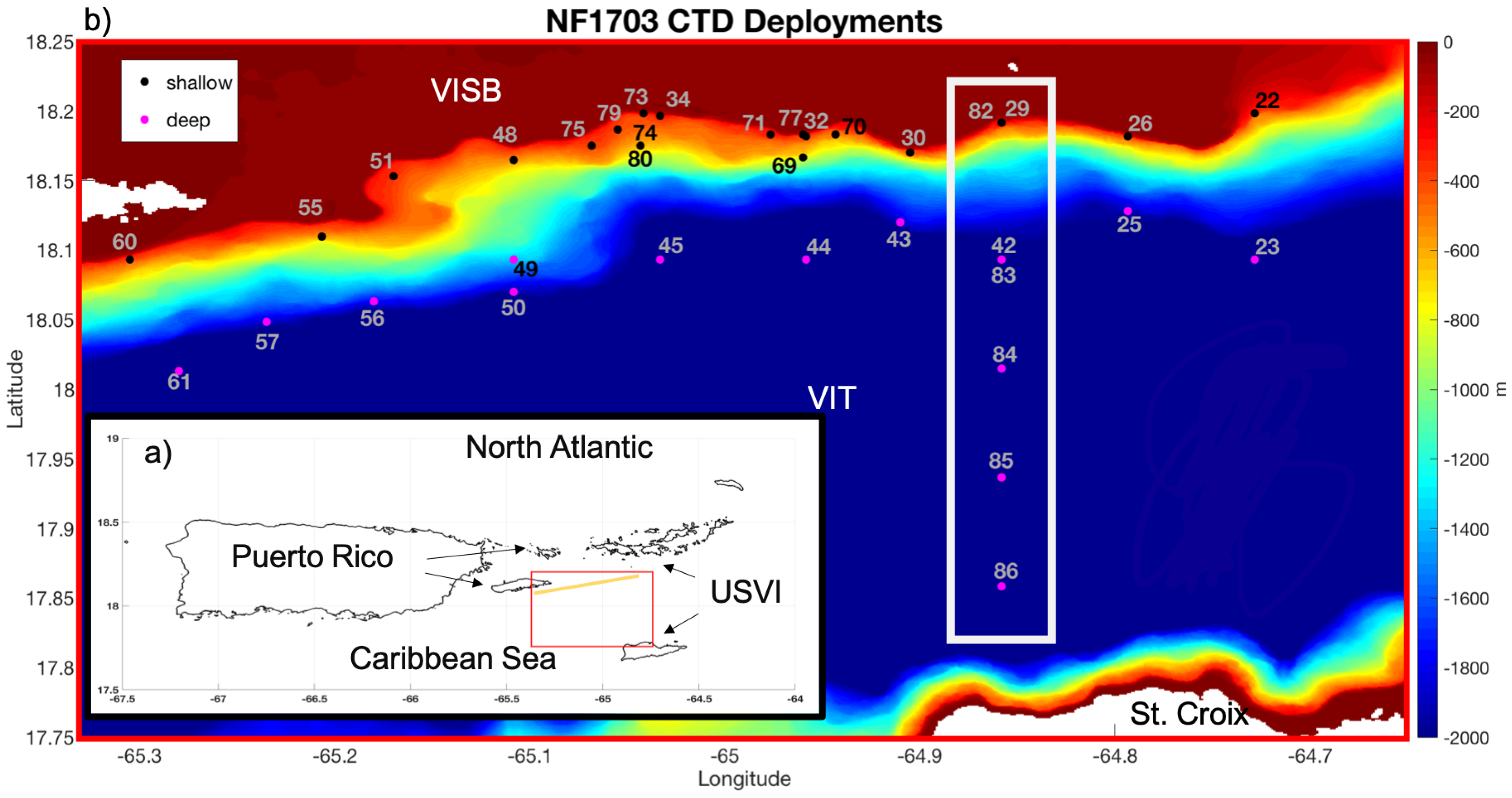
Figure 1. (a) Map of the area, with red box showing the study region enlarged in panel b and yellow diagonal line indicating the approximate location of the shelf break. (b) Bathymetry contours limited to 2000 m for the study area obtained from National Oceanic and Atmospheric Administration (NOAA) National Geophysical Data Center Coastal Relief Model and locations of Conductivity–Temperature–Depth (CTD) casts (identified by their chronological number during the sampling); shallow (black dots) and deep (magenta dots). Three main transects are used in the analysis: along-shelf shallow transect of stations along the shelf break (black dots), along-shelf deep transect of stations just after the shelf break (magenta dots along the shelf break), and stations along the North–South transect in the cross-shelf direction enclosed by the white rectangular box.
Jmse 07 00074 g001
Figure 2. Characteristic profiles of: (a) temperature, (b) density, and (c) salinity. Black profiles correspond to shallow stations and magenta profiles to deep stations.
Jmse 07 00074 g002
Figure 3. Depth of Salinity maxima for Stations 60, 48, and 22 (shallow), and 61, 50, 23 (deep).
Jmse 07 00074 g003
Figure 4. (a) Temperature, (b) density, (c) salinity, and (d) relative Chlorophyll-a (Chl-a) profiles for North–South transect stations. Color represents the location of each profile by latitude.
Jmse 07 00074 g004
Figure 5. (a) Difference from mean density profile of North–South transect stations, and (b) Difference from mean salinity profile of North–South transect stations.
Jmse 07 00074 g005
Figure 6. (a) Temperature, (b) density, (c) salinity, and (d) relative Chl-a profiles for shallow stations. Color represents their location by longitude.
Jmse 07 00074 g006
Figure 7. (a) Temperature, (b) density, (c) salinity, and (d) relative Chl-a profiles for deep stations. Color represents their location by longitude.
Jmse 07 00074 g007
Figure 8. Standard deviations for shallow and deep station profiles: (a) Temperature, (b) Density, and (c) Salinity.
Jmse 07 00074 g008
Figure 9. Temperature–Salinity diagrams from all sampled stations and different water masses in the region: Caribbean Surface Water (CSW), Subtropical Underwater (SUW), Sargasso Sea Water (SSW), Tropical Atlantic Central Water (TACW), Antarctic Intermediate Water (AAIW), and North Atlantic Deep Water (NADW). Colors represent (a) dissolved oxygen [mg/L] and (b) depth [m]. TS diagrams were generated using Ocean Data View [27].
Jmse 07 00074 g009
Figure 10. Satellite derived Chl-a concentrations from 30 March to 9 May 2017. Data obtained from the NASA GES DISC GIOVANNI tool [29].
Jmse 07 00074 g010
Table 1. Station classification.
GroupStations
Shallow22, 26, 29, 30, 32, 34, 48, 51, 55, 60, 69, 70, 71, 73, 74, 75, 77, 79, 80, 82
Deep23, 25, 42, 43, 44, 45, 49, 50, 56, 57, 61, 83
North–South82, 83, 84, 85, 86
Table 2. Ranges of temperature, density, and salinity for shallow and deep stations averaged by depth intervals.
Range ofRange ofRange of
GroupTemperatureDensitySalinity
[ C][kg/m3][PSU]
Shallow (0–50 m)0.250.220.2
Deep (0–50 m)0.330.230.17
Shallow (51–100 m)1.030.540.30
Deep (51–100 m)0.400.240.18
Shallow (101–200 m)2.020.550.25
Deep (101–200 m)0.840.250.11
Shallow (201–300 m)1.230.160.20
Deep (201–300 m)0.970.120.16
Table 3. Water masses and approximate range of their defining characteristics.
Water MassDepth RangeTemp. RangeSal. RangeOxygen RangeDens. Interface
[m][ C][PSU][mg/L]
CSW0–100>2436.2–37>5.5>25
SUW100–20020–25>37>5.525–26
SSW200–40014–2036–374.7–5.526–27
TACW400–7508–1435.3–364–4.726–28
AAIW750–10005–834.7–35.33.8–427–28
NADW>1000<634.7–35>4>27

