Article

The Snell’s Window Image for Remote Sensing of the Upper Sea Layer: Results of Practical Application

Institute of Applied Physics of the Russian Academy of Sciences, 46 Uljanova St., 603950 Nizhny Novgorod, Russia
*
Author to whom correspondence should be addressed.
J. Mar. Sci. Eng. 2019, 7(3), 70; https://doi.org/10.3390/jmse7030070
Submission received: 28 February 2019 / Revised: 12 March 2019 / Accepted: 15 March 2019 / Published: 19 March 2019
(This article belongs to the Special Issue Underwater Imaging)

Abstract

:
Estimation of water optical properties can be performed by photo or video registration of rough sea surface from underwater at an angle of total internal reflection in the away from the sun direction at several depths. In this case, the key characteristic of the obtained image will be the border of the Snell’s window, which is a randomly distorted image of the sky. Its distortion changes simultaneously under the action of the sea roughness and light scattering; however, after correct “decoding” of this image, their separate determination is possible. This paper presents the corresponding algorithms for achieving these possibilities by the Snell’s window images. These images were obtained in waters with different optical properties and wave conditions under several types of illumination. Practical guidelines for recording, processing and analyzing images of the Snell’s window are also formulated.

1. Introduction

The underwater sky image, or the Snell’s window, is a contrasting object frequently observed in photos of professional and amateur divers alike (Figure 1). However, the use of such images to solve scientific problems has not been noticed until recently.
For a flat sea surface, the Snell’s window looks like a light circle with an angular radius equal to the angle of total internal reflection of 48.75° (Figure 1a). An apparent radiance of the sea surface at angles more than 48.75° is determined through the upwelling light reflected by water boundary to the lower hemisphere. In fact, the upwelling radiance is too low in comparison with the downwelling one; therefore, the apparent radiance of the surface beyond Snell’s window appears to be comparatively low. Surface waves randomly distort the border of the Snell’s window resulting in the appearance of lots of dark and light spots near it (Figure 1b). Thus, contours of light and dark spots around the Snell’s window border outline the surface patches where the slope exceeds the certain value depending on spot location. This opens up possibilities for retrieval of the slope distribution function or its parameters like slope variance by distortions of the Snell’s window border. The effects of multiple scattering and absorption of light in water also affect the distortion of the Snell’s window border, getting stronger with depth increase (Figure 1b,c).
The first images of the Snell’s window for estimation of sea roughness parameters were obtained in the Black Sea in 2010 during the photo registration of the underwater solar path at the time of sunset. In this case, the sun solar path was near the border of the of Snell’s window. Its study allowed us to establish that the Snell’s window border is very sensitive to the sea surface roughness and can be used to determine its statistical properties [1]. The first algorithm for estimating the slope variance by value of its border distortion in case of slope less than 20° was proposed in [2]. Similar estimation for roughness with breaking waves based on the roughness representation as a sine curve with known characteristics was obtained in [3]. Subsequently, on the basis of a simplified model of the Snell’s window [4], a new algorithm for reconstructing the wind-waves frequency spectra was developed [5]. On the one hand, it was assumed that both algorithms were applicable at optical depths less than one, where the effects of light scattering and absorption can be neglected. On the other hand, it created the background for determining the optical properties of water at greater depths. As a result, in [6], the outcome of the theoretical study in estimating the absorption and scattering coefficient of water through the Snell’s window distortion was presented under the assumption that there was a known parameter, characterizing sea roughness like slope variance. Results of the first testing of the proposed algorithms for images from the Black Sea and empirical regressions between the inherent optical properties (IOP) at 532 nm [7] are presented in [8]. Subsequently, the possibility of determining the absorption coefficient for three spectral channels (420 nm, 530 nm and 650 nm) was demonstrated for fresh water of the Gorky Reservoir, characterized by high concentrations of chlorophyll a and dissolved organic matter [9].
The scope of the present investigation was aimed at estimating both the characteristics of the sea roughness and the optical properties of water for both its types (Case 1 and Case 2), for different illumination and sea roughness conditions and without applying empirical regressions between IOP. In addition, practical recommendations of the Snell’s window image registration, processing and analysis will be made in this work.
Additionally, we would like to note that the emphasis on our own research in this article is connected with the fact that there have been no similar results from other research teams. The analysis of modern studies on using Snell’s window image for estimating characteristics of the upper water layer confirms the assertion made. At the present time, a great number of methods, approaches and techniques for studying the sea surface parameters and the optical properties of water have been developed; however, we were interested in the possibility of specifically using underwater images for this purpose.

2. Materials and Methods

The work was based on the theoretical model of the accumulated Snell’s window image [8,10], the proposed algorithms for solving inverse problem and the data of field measurements from several expeditions of 2018. For a better understanding of the paper we will briefly consider the theoretical model of the instantaneous image of the Snell’s window, explain the physical principles of its formation and provide a table of abbreviations and symbols used in this paper (Table 1).

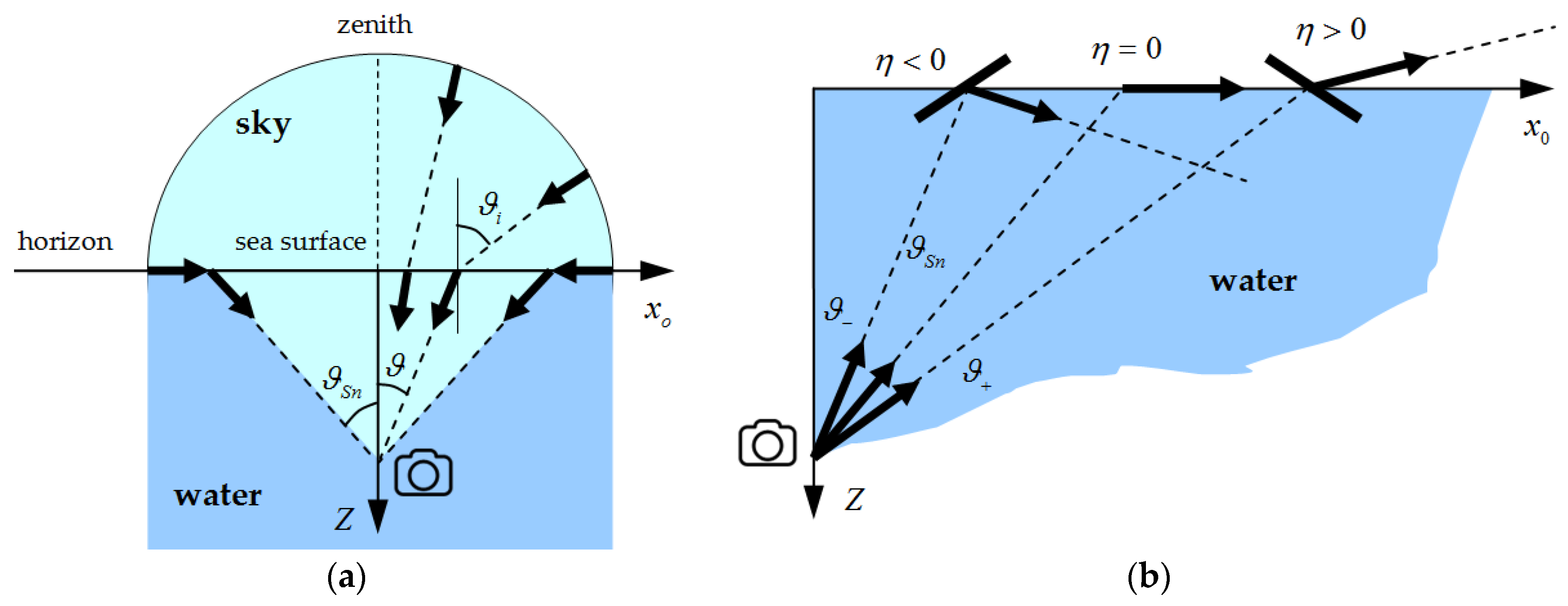
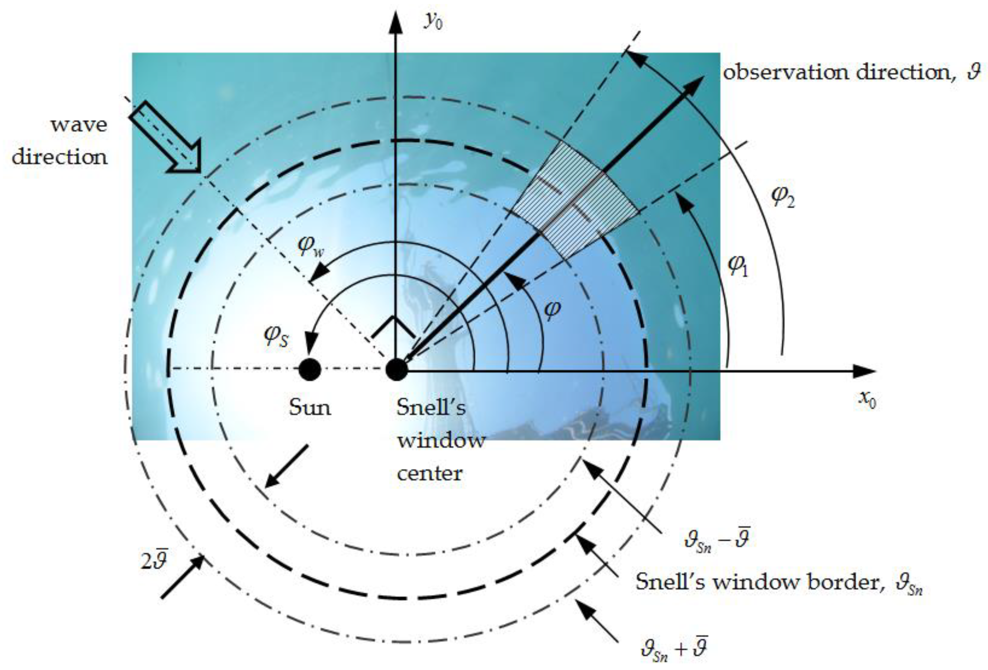
2.1. Analytical Model of the Instantaneous Snell’s Window Image Formed by Nonscaterred Light

When we constructed the instantaneous Snell’s window image model (see details in [2]), we assumed that it is formed using an ideal optical system placed at depth Z that records the angular radiance distribution of the sea surface (Figure 2a). The equations for calculating this radiance were derived in the geometrical optics approximation, mathematical instrument of the radiation transfer theory for turbid water and the boundary conditions for the intensity of light that transfers between mediums with different refraction indexes (air-water). At the same time, we took into account the effects of multiple instances of light scattering and absorption; however, effects of light backscattering were neglected. Optical properties of the water are characterized by absorption coefficient a , scattering coefficient b and phase function x ( γ ) , where γ is a scattering angle. Elevations of sea surface ζ and its slopes η = ζ / 1 + ( ζ ) 2 were assumed to be stationary and homogeneous Gaussian random fields, which allowed us to use corresponding surface slope distribution function P ( η , σ x 2 ) with a single parameter—the slope variance σ x 2 (for one-dimensional case). The influence of surface elevations ζ on the structure of the light field at depth Z ζ was considered negligible. Surface slopes were small and there was no shadowing.
Neglecting the effects of light scattering in water, instantaneous radiance of the sea surface element, observable at angle ϑ from depth Z at time moment t , is determined by the equation:
I o ( ϑ , Z , t ) = m 2 [ 1 R F ( α ( ϑ , t ) ) ] I s k y ( ϑ i ( ϑ , t ) ) e c Z / cos ϑ ,
where m is the refraction index, c is the attenuation coefficient, I s k y is the sky luminance distribution, ϑ i is the local incident angle,
R F ( α ( ϑ , t ) ) = 1 2 [ ( 1 α ( ϑ , t ) 2 m 2 α ( ϑ , t ) 2 1 α ( ϑ , t ) 2 + m 2 α ( ϑ , t ) 2 ) 2 + ( 1 α ( ϑ , t ) 2 m 2 m 2 α ( ϑ , t ) 2 1 α ( ϑ , t ) 2 + m 2 m 2 α ( ϑ , t ) 2 ) 2 ]
is the Fresnel reflection coefficient for a non-polarized light and
α ( ϑ , t ) = sin ϑ i ( ϑ , t ) = m ( sin ϑ cos ϑ η ( x ( ϑ ) , t ) )
is the sinus of the local incident angle ϑ i which is a function of observation angle ϑ and surface slope η at point x = Z tan ϑ and time moment t .
According to Equations (1)–(3) the structure of the Snell’s window image for certain relief of the sea surface is determined by several factors: the nature of its lighting; radiance attenuation of light penetrating into the water due to its reflection from sea surface; change of light direction when it is penetrating through the surface; and light attenuation on the way from the surface to the receiver.
In the absence of wind roughness, when η = 0 , a horizontally incident light according to Equation (3) is refracted at an angle:
ϑ = ϑ S n = arcsin ( 1 / m ) 48.75 °
and the surface radiance in this direction is close to zero according to Equation (5). In a two-dimensional case, we obtain the cone of such rays with angular radius ϑ S n . The “intersection” of this cone with a flat sea surface forms the circle border which is a border of the Snell’s window. At the initial depth interval, the apparent radiance of the surface inside the border is determined by the sky luminance distribution I s k y and the transmittance dependence 1 R F . Outside the Snell’s window, the image was formed by backscattering from the water column and light refracted downward by the sea surface, the radiance of which is relatively small. Therefore, the Snell’s window looks like a light circle on a dark background (see Figure 1).
Surface waves randomly distort the Snell’s window: dark spots appear inside of it, light spots—outside. The mechanism of their appearance is explained in Figure 2b. Angles ϑ S n , ϑ and ϑ + show the directions to the undisturbed Snell’s window border, and to dark and bright spots, respectively. As shown in Figure 2b, bright spots outside the undisturbed Snell’s window appear in places of the surface with a positive slope (slope towards the horizon) through which the observer sees fragments of the sky. At the same time, dark spots inside the undisturbed Snell’s window appear on the surface elements with a negative slope, through which the sky is not visible. The number of spots, their sizes and occupied area depends on the intensity of waves. The last one can be estimated on the basis of the accumulated Snell’s window image L 0 , which is calculated through the instantaneous radiance of the sea surface I and the surface slope distribution function P ( η , σ x 2 ) :
L 0 ( ϑ , Z , σ x 2 ) = 1 1 I ( ϑ , Z , η ) P ( η , σ x 2 ) d η
Obviously, this image depends on the sea surface state, on the basis of which the algorithm to restore the slope variance [2] was developed. In writing Equation (5), the time argument t of function I ( ϑ , Z , t ) is replaced by surface slope η in view of the fact that η = η ( t ) .

2.2. Analytical Model of the Accumulated Snell’s Window Image Taking into Account Scattering Properties of Water

The model of the accumulated Snell’s window image takes into account the effects of multiple scattering and absorption of light in water is quite voluminous and has already been presented in previous work [8,10]. Therefore, in this paper, we present only the general equations that are necessary for the description and implementation of algorithms for the restoration of water optical properties; moreover, we specify the conditions for their derivation and their applicability.
According to this model, the radiance of the accumulated image of the Snell’s window L as a function of polar angle ϑ and depth Z can be calculated by the equation:
L ( ϑ , Z , a , b , σ x 2 ) = A ( ϑ , Z , a ) [ L ( ϑ , Z , b , σ x 2 ) ] a = 0
where:
A ( ϑ , Z , a ) = exp [ ( a Z / cos ϑ ) ]
is the first function which takes into account the influence of absorption on the Snell’s window image, and:
[ L ( ϑ , Z , b , σ x 2 ) ] a = 0 = 1 π 1 1 L 0 ( arcsin ( cos ϑ n x sin ϑ ) , Z , σ x 2 ) 0 exp [ b Z cos ϑ ( 1 x s ( p ) ) ] cos ( n x p ) d p d n x
is the second function that describes the structure of the image in hypothetical water medium without absorption. Here, x s ( p ) is the spectrum of phase function x ( γ ) . Equation (8) is obtained by using the Green function in the small-angle diffusion approximation [11].
The proposed model is applicable when the following conditions are met:
(1) Light field L should be horizontally uniform in water column with cross size Δ x > Δ x 0 5 Z ;
(2) Depth Z should be such that the additional light beam after passing through the layer of thickness Z / cos ϑ s remains sufficiently narrow.
As we can see from Equations (6)–(8), function L depends on three parameters: absorption and scattering coefficients a and b , and slope variance σ x 2 . The first of which is included only in the multiplier A ( ϑ , Z , a ) and two others in multiplier [ L ( ϑ , Z , b , σ x 2 ) ] a = 0 . Examples of calculating these functions are shown in Figure 3, wherein the sky luminance distribution was considered uniform and the water surface was flat. Radiance of the surface elements, observable at angles more than the angle of total internal reflection is considered equal to zero. Light scattering in water was given by the well-known phase function [11,12]:
x ( γ ) = 2 2 / d x γ 1 exp ( 2 / d x γ )
where d x is the variance of a single scattering angle. The phase function (9) has been used in a lot of works on the theory of underwater vision [11]. With appropriate values of parameter d x it describes well the form of real seawater phase function in the range of scattering angles 0.5 0 < γ < 30 0 ÷ 45 0 .
Figure 3a shows that with increasing depth apparent radiance of the Snell’s window decreases and its border blurs. At the same time, according to Figure 3c, all curves intersect at angle ϑ = ϑ S n . This means that light scattering in water does not affect the apparent radiance of the Snell’s window border and, therefore, its radiance is attenuated with depth only due to absorption. In reality, a certain dependence on the turbidity should be observed, at least due to the backscattering of light in water, which has not been taken into account. In addition, when deriving Equations (6)–(8), the distortion of the Snell’s window border was implicitly likened to the distortion of luminous half-plane border, which could also lead to some error in estimating the effect of scattering on the apparent radiance of the Snell’s window border. However, under condition d x b Z < < cos ϑ S n , this effect should not be significant, which creates the prerequisites for constructing simple algorithms for the separate determination of the absorption and scattering coefficients of water by radiance attenuation of the Snell’s window border and a parameter characterizing its distortion.

2.3. Algorithms for Solving Inverse Problems

If we assume that the attenuation of the apparent radiance of the Snell’s window border is completely determined by function A ( ϑ , Z , a ) , then the absorption coefficient can be expressed as:
a = cos ϑ S n Z 2 Z 1 ln L ( ϑ S n , Z 1 , a , b , σ x 2 ) L ( ϑ S n , Z 2 , a , b , σ x 2 )
through the radiances at two different depths Z 1 and Z 2 at angle ϑ S n coinciding with the direction to the Snell’s window border. Subsequently, we will use the value:
Z = Z 2 Z 1
to determine thickness of the water layer between horizons Z 1 and Z 2 . After that, with known absorption coefficient and measured radiance distribution L ( ϑ , Z , a , b , σ x 2 ) , we can find the auxiliary function:
[ L ( ϑ , Z , b , σ x 2 ) ] a = 0 = L ( ϑ , Z , a , b , σ x 2 ) A ( ϑ , Z , a )
which depends on the scattering coefficient and slope variance. If the last parameter is known, the scattering coefficient of water can be recovered in two ways [8]:
(1) By introducing the parameter characterizing the value of the Snell’s window distortion, and determining the scattering characteristics by fitting the theoretical value of this parameter to the experimental one (Algorithm 1);
(2) By calculating the parameter characterizing contrast of variations in the apparent radiance of the Snell’s window in a given interval of angles near its border (Algorithm 2).
Estimation of the efficiency of each proposed algorithm was carried out on the basis of experiment data, and its results are presented below.

2.4. Experiment

In 2018, full-scale measurements were performed in the Black Sea and in the Gorky Reservoir. A Logitech C210 webcam with 30° field of view in the underwater box was used to record the Snell’s window images. On its front panel, three replaceable color filters were mounted: a red filter (band 560–2500 nm with no peak), a green filter (band 460–620 nm with peak 530 nm) and a blue filter (band 380–520 nm with peak 420 nm). Images resolution was 1280 × 720 pixels, recording frequency—15 frames per second. The camera was remotely controlled in online mode. Replacement of the color filter was carried out physically after performing measurements at all depths with the chosen color filter.

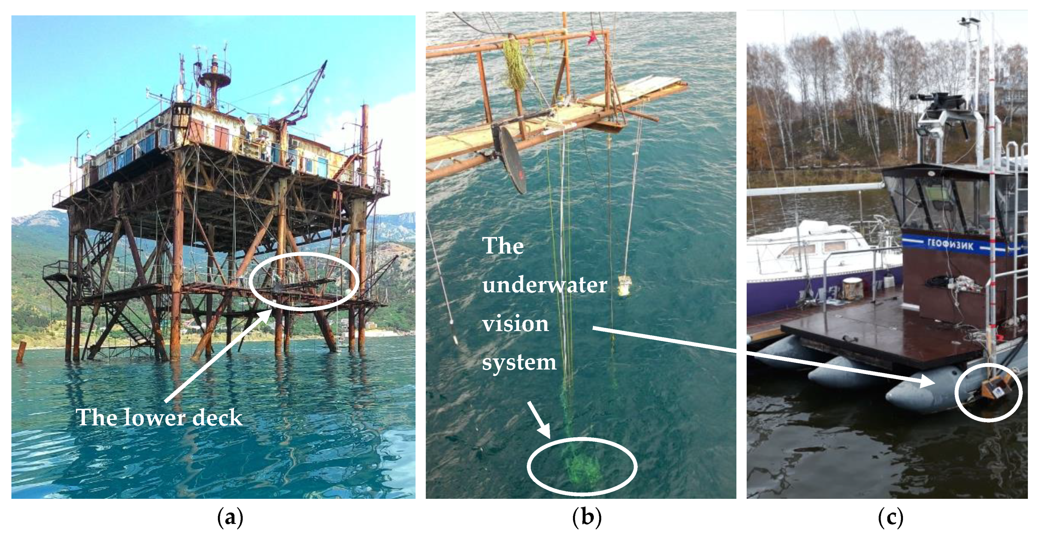
2.4.1. The Black Sea Experiment

The Snell’s window images were recorded in October of 2018 from the Oceanographic Platform of the Marine Hydrophysical Institute, which is based in 600 m off the seashore (Figure 4a). The box with webcam was attached to a triangular rigid metal frame at angle ϑ S n , which was lowered from the lower deck of the platform along the stretched cable. The first depth was 0.5 m and the last one 6.5 m; depth increment was 1.0 m. Adjustment and fixation of the camera on the azimuth angle was carried out by lateral stretch marks (Figure 4b). Video recording was performed on each horizon for 3 minutes with subsequent transition to the next depth within 1 minute. Therefore, a full measurement cycle on seven horizons for one color filter took about 30 minutes. The first video recording in the green color filter was started at 11:34 AM, then after 50 minutes in red color filter and after a long break for 2 hours in blue color filter. During this time, according to the data from digital anemometer Windsonic, the wind speed decreased from 5–6 m/s at 10:00 AM to 3–5 m/s at 11:30 AM, and at 12:00 PM, the wind completely faded. At the same time, fading swells were observed on the sea surface; their amplitude was about 0.4 m at 11:00 AM and became barely noticeable at 15:00 PM. The swell characteristics were estimated visually by the marks on the supporting piles of the platform at the time of passage. These waves had a noticeable effect on camera oscillation, which was later eliminated during image processing. The sky was clear throughout the day. Simultaneously with the video recording, the vertical profiles of the attenuation coefficient were measured using submersible multichannel optical sonde [13] working at 460 nm, 532 nm and 625 nm; wind speed and direction were measured using the ultrasonic digital anemometer WindSonic and sky radiance distribution was measured using digital camera Nikon D5100 with 10.5 mm f/2.8 G ED DX Fisheye-Nikkor lens, which provided 180° field of view.

2.4.2. Gorky Reservoir Experiment

A similar work was performed in eutrophic fresh waters of the Gorky Reservoir in the late autumn of 2018 during residual cyanobacteria bloom. The box with webcam was fixed to an aluminum pipe at angle ϑ S n that was lowered from the deck of the anchored vessel (Figure 4c). The first depth was 0.5 m and the last one 2.0 m; depth increment was 0.25 m. Video recording of 60 second was 0.5 m and the last one 2.0 m; depth increment was 0.25 m. Video recording of 60 second was performed on each horizon; full measurement cycle took under 8 minutes. The maximum depth was comparable with the Secchi depth. Wind and waves were absent; the sky was overcast.
Concurrent measurements of the scattering coefficient at 532 nm were performed by a turbidity meter model Turbido-1M [14]. Determination of the spectral absorption coefficient was implemented in the laboratory on the basis of selected water samples using a double beam spectrophotometer and integrating sphere to increase the optical path length [15].
General information on the roughness, optical properties of water and sky conditions on the measurement days is presented in Table 2.

3. Results and Discussion

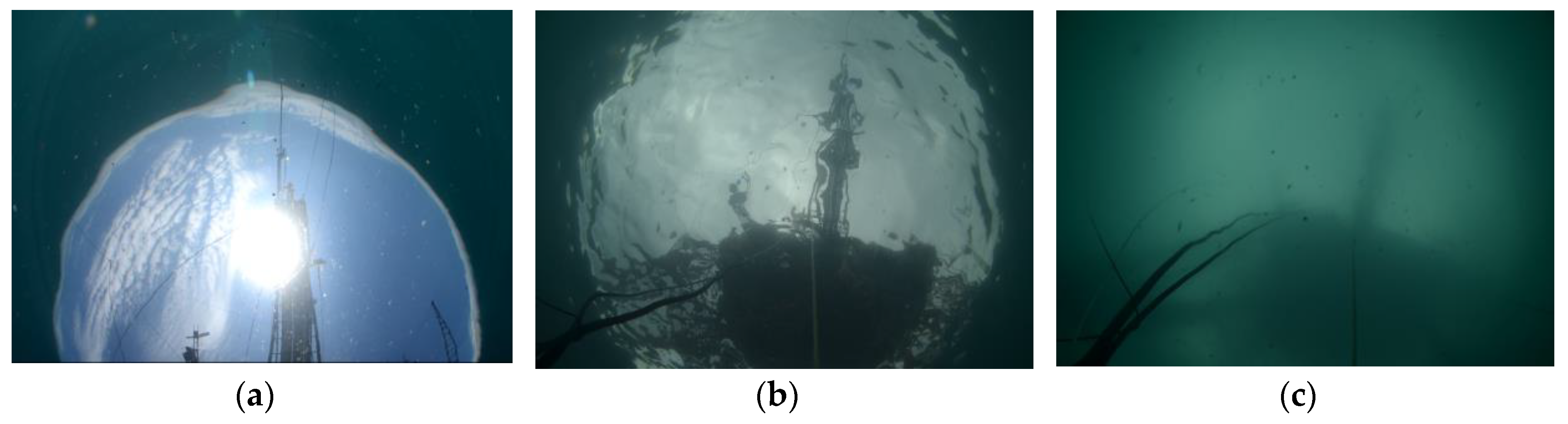
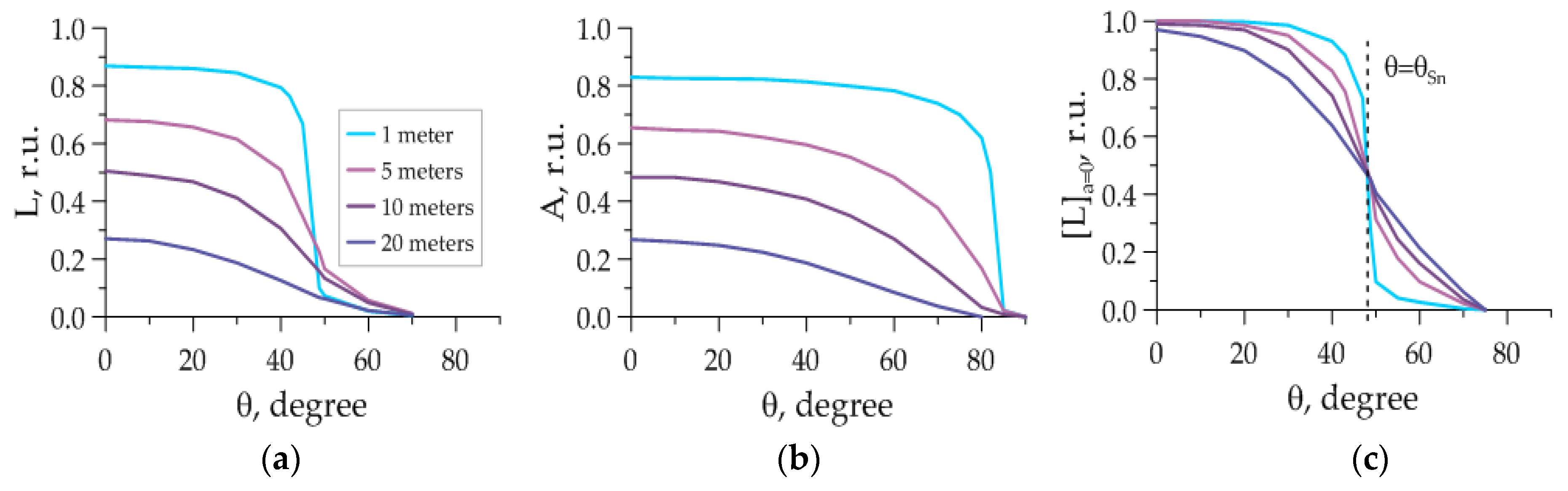
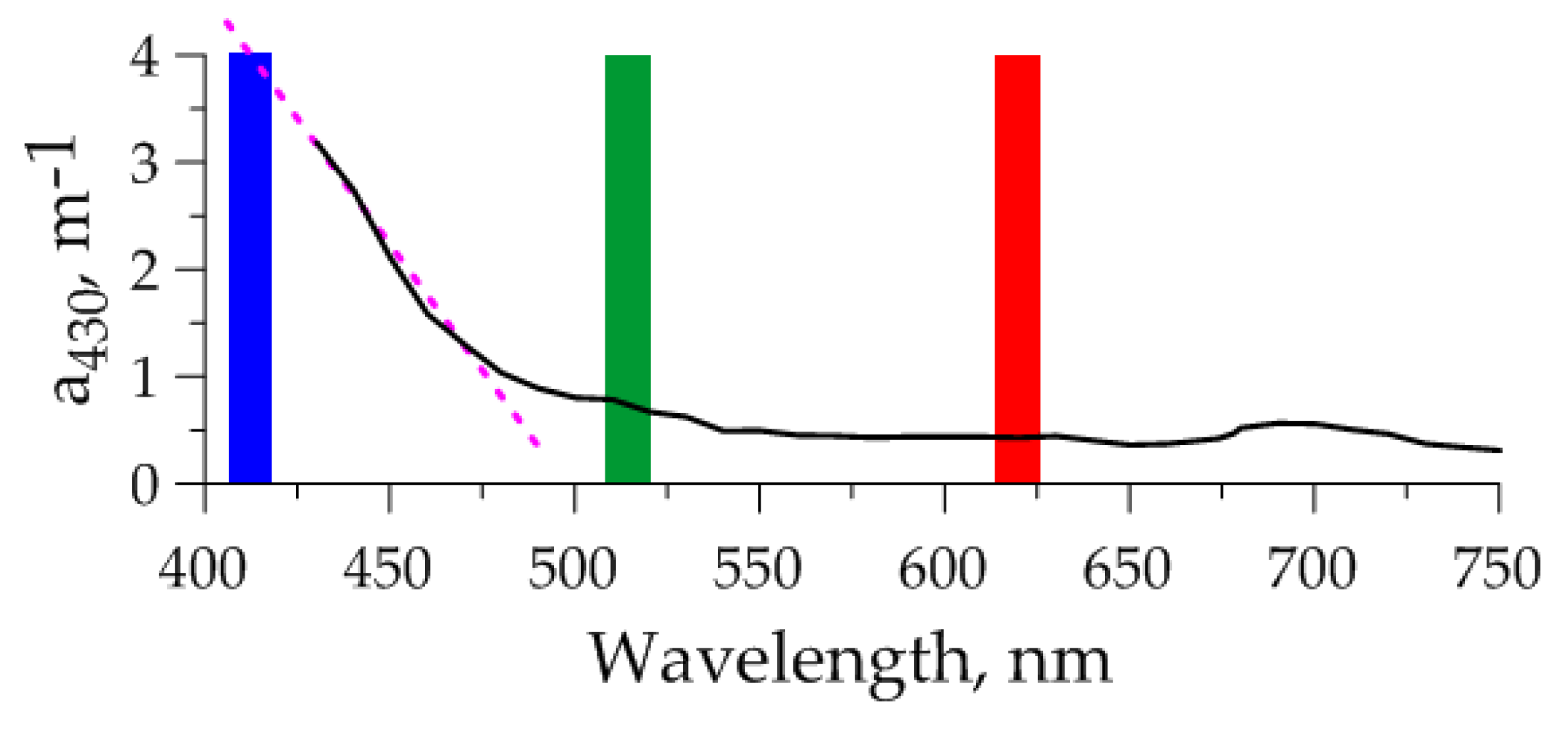
3.1. Selection of the Optimal Section of the Snell’s Window Image

The trial registration of the Snell’s window images was used to assess the surface waves characteristics. If the greater surface area was captured, then the chance for full and accurate estimate of surface roughness parameters was higher. However, in the case of swell waves or developed wind waves with the selected direction, the estimate of slope variance or roughness frequency spectrum could be obtained by section of the Snell’s window in the general direction of the surface waves. This section can be used to recover the optical properties of water according to [6,8,9]; however, it is a suboptimal choice. Figure 5 demonstrates the selection of the optimal section of the Snell’s window on the example of its image obtained at the depth of 1 m with Nikon D5100 fisheye-Nikkor lens 10.5 mm f/2.8 G ED DX in the waters of the Black Sea on a clear day with small sea surface roughness. The direction of the waves propagation and Sun position were set by azimuth angles φ w and φ S . The optimal section φ will be the section that is oriented perpendicular to the direction of wave propagation, lying within angular region of 90° to 270°, relative to the direction to the Sun. Implementation of the first condition allows to minimize the distortion of the Snell’s window border due to the surface waves, and the second allows to avoid light exposure and sun glint.
In practice, it seems that the existence of still milder conditions is possible, namely, in the analysis of the section of the Snell’s window in a certain range of angles ± ϑ ¯ near direction ϑ S n (dotted circles in Figure 5). Interval ϑ [ ϑ S n ϑ ¯ : ϑ S n + ϑ ¯ ] is determined by double mean angle ϑ ¯ of distortion of the Snell’s window border under surface waves and light scattering in water. According to estimates from [3] maximum of ϑ ¯ is about 8° for winds of 10 m/s. If we assume that light scattering in water has the same impact on the distortion of the Snell’s window, the total distortions 4 ϑ ¯ by waves and light scattering will be about 30°. This means that optical receivers with a viewing angle of 30° or more can be used for recording of the Snell’s window images. The simplest device, such as a webcam, satisfies this condition; therefore, we used one in our full-scale experiments.
In addition to the choice of the optimal cross section of the Snell’s window, there was a question regarding the number of sections needed to restore water optical properties or sea waves parameters. From practical experience, reliable results of water optical properties restoration were obtained by processing of at least one minute videos at a frame rate of 15 frames per second. This is processing of 1000 frames. Similar number of sections can be obtained from a single frame by using radial sections in the sector of azimuth angles φ [ φ 1 : φ 2 ] marked by shaded area in Figure 5. The exact number of sections was set by the resolution of the optical receiver: starting from 480 pixels for the webcam up to 6000 pixels for the SLR camera. The following results, based on the analysis of video recordings of several expeditions, assess the real possibilities of webcam implementation as comprehensible optical receiver.

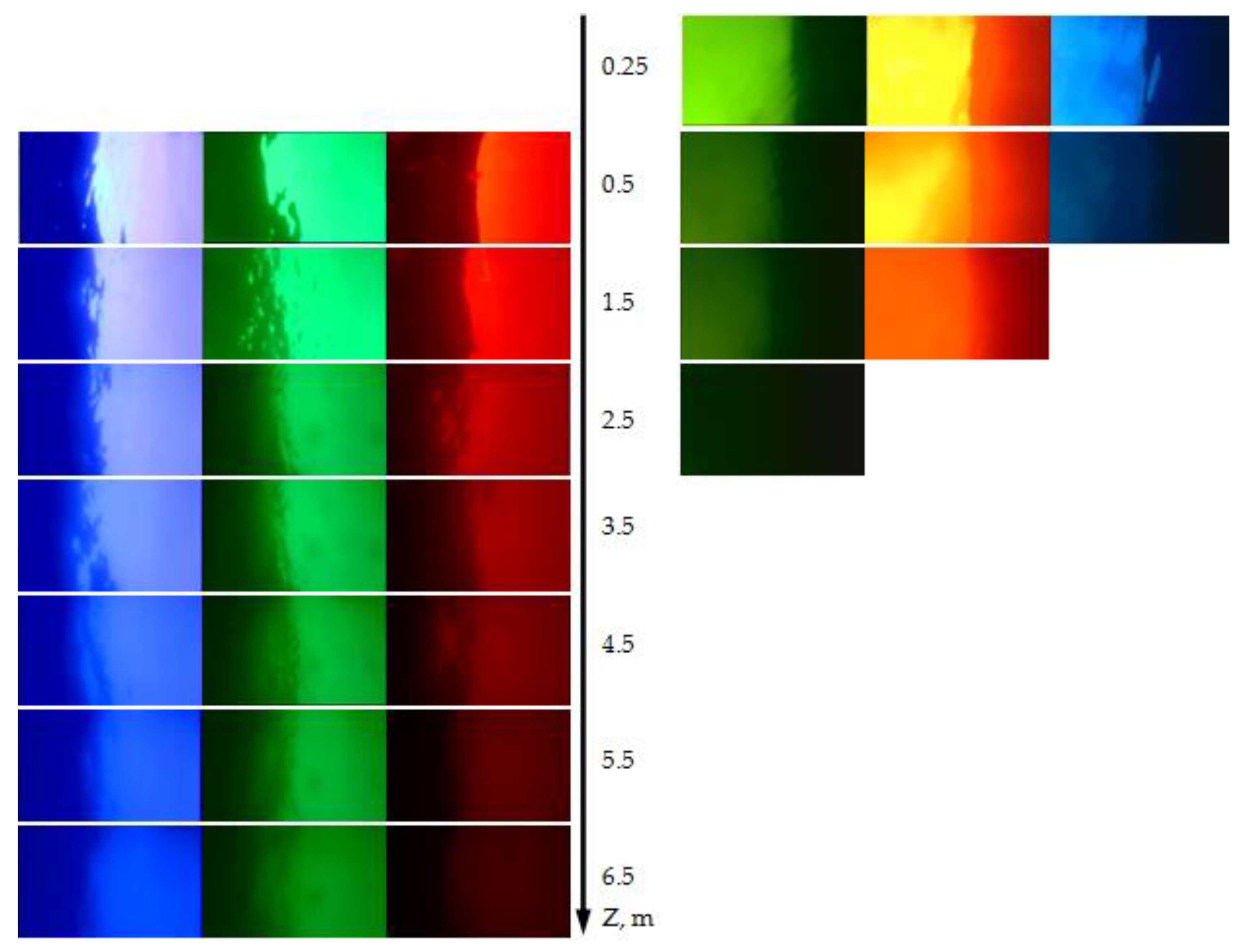
3.2. Image Processing Technique

Figure 6 shows instantaneous images of the Snell’s window, registered in three color filters on seven horizons in the Black Sea (on the left) and the Gorky Reservoir (on the right), by the abovementioned webcam. It can be seen that the radiance of the images in sea water in the blue and green filters decreased in depth approximately at the same pace, whereas the radiance of the image in the red filter decreased more rapidly. In eutrophic fresh waters, the greatest decrease was observed in blue color due to its absorption by dissolved organic matter, average concentrations of which for the Gorky Reservoir are 13 mg/L. Therefore, the depth limit of visibility of the Snell’s window in blue color did not exceed 1.5 m while the depth limit of visibility for green color was 2.5 m, close to the Secchi depth.
Images from Figure 6 were used to recover the waves characteristics and the water optical properties. The algorithm of their processing is as follows:
  • 21 videos, recorded at seven depths in three color filters, were loaded into specially developed software. Each video was divided into frames and an array of frames with dimensions p x × p y × N i , j was formed, where p x = 1280 and p y = 720 are resolutions along the Snell’s window image and across it, respectively, N i , j is the frame number of video according to depth Z i , i = [ 1 : 7 ] and each color filter, where j = [ 1 : 3 ] is a number of color.
  • Correct calculation of the statistical characteristics of the Snell’s window image could be performed only on the basis of data arrays of a uniform dimension. As each video had its own duration the following search procedure of video with minimum length was used:
    N ¯ = min { N i , j }
    with the subsequent shortening of the original arrays to dimension p x × p y × N ¯ i , j , where N ¯ i , j = N i , j ( 1 : N ¯ ) .
  • Then, cycle n = 1 : N ¯ was started and ach frame was averaged in cross direction along the transverse coordinate p y . As a result, the array p x × N ¯ i , j of accumulated radial cross section image of the Snell’s window was formed.
  • For each accumulated radial cross section the search of the Snell’s window border was carried out by its sliding window smoothing with subsequent differentiation by p x :
    d L i , j ( p x ) = d d p x L i , j ( p x ) ,
    where index i still corresponds to depth and j —to number of color filter. In Equation (14) variable Z is derived from the number of arguments of initial function L (see Equation (6)) in connection with its introduction to the corresponding index i . Also the viewing angle ϑ is replaced to the pixel coordinate p x . Other remaining parameters are omitted for compact representation. The function minimum (14) corresponded to the Snell’s window border p i , j , n S n . This procedure was necessary, as the webcam was not rigidly fixed underwater and, as a result, was slowly rocking due to current and wind-wave action. The knowledge of the Snell’s window border coordinates made it possible to center each section relative to it.
  • The location of the Snell’s window border in the left or right half of the image determined the distance to the image edge p i , j , n = min ( | p i , j , n S n p 1 | ; | p i , j , n S n p 720 | ) . Minimizing the array of coordinates of the Snell’s window border over all sections allowed to calculate the minimum value Δ p ¯ = min i , j , n p i , j , n , and cut off all sections, reducing them to a single scale. [ Δ p ¯ + p i , j , n S n : p i , j , n S n + Δ p ¯ ] . In other words, all the Snell’s window sections were limited to single scale images with a centered border of the Snell’s window. This allowed us to minimize the influence of camera rocking and ensure the Snell’s window imaging validity from all expeditions. In cases where camera rocking was significant due to long waves, the data was discarded.
  • The final step was the normalization of each section by radiance at first depth and pixel with coordinate p x = 10:
    L i , j , n ( p x ) = L i , j , n ( p x ) / [ L i , j , n ( p x ) ] | i = 1 .
It is worth noting that we intentionally retreated from the edge of the section by 10 pixels for the purpose of eliminating the influence of image edge effects.

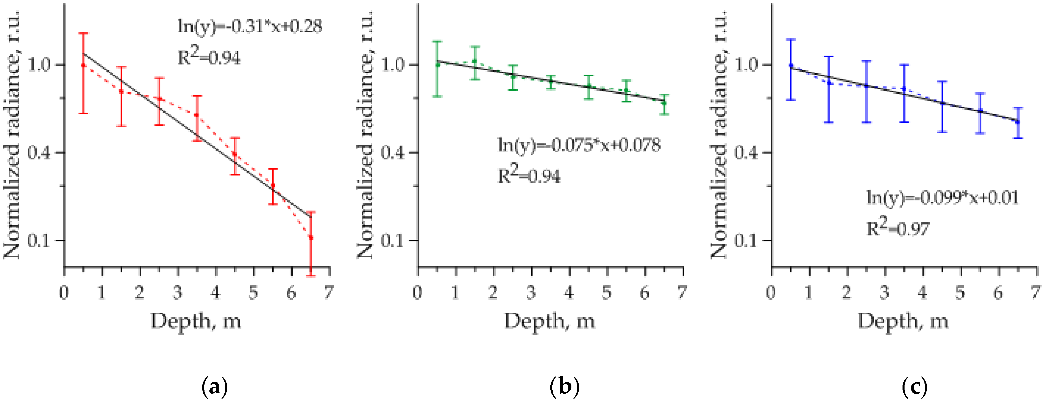
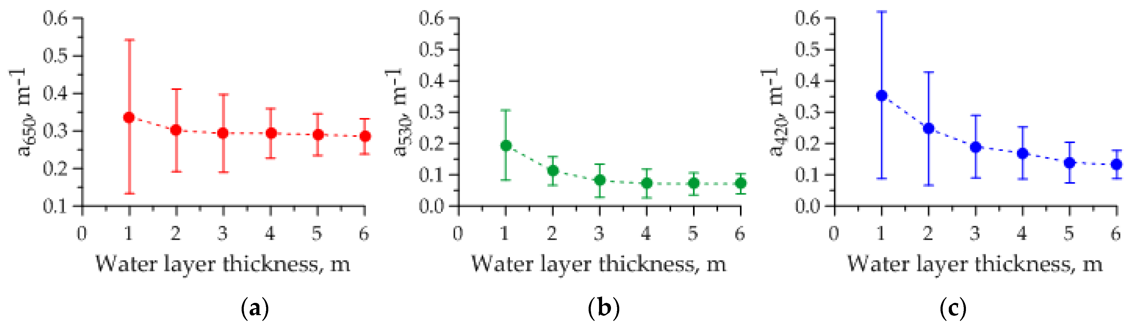
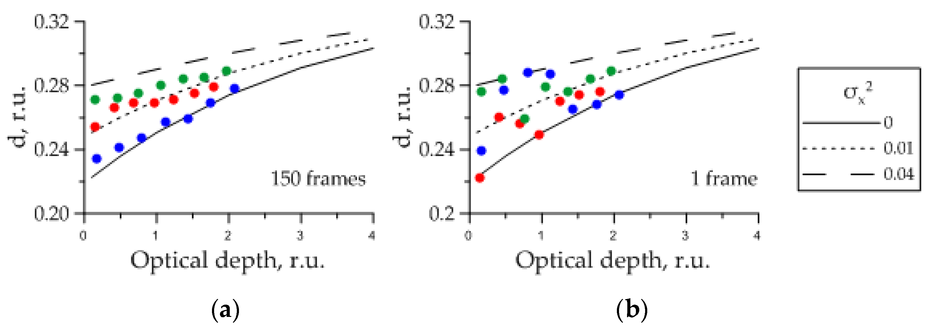
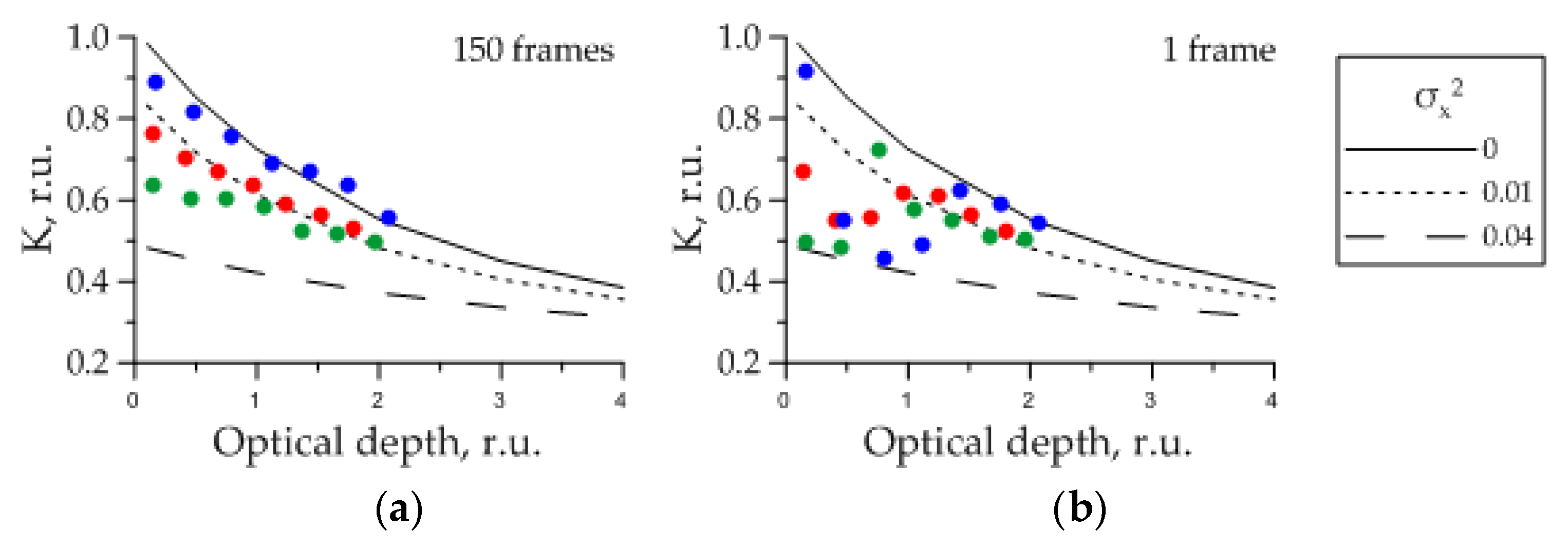
3.3. Determination of Absorption Coefficient

Firstly, let us consider possibilities of a single frame for each depth and color filter. We will assume that for each frame, all preparatory actions from the previous section have been completed. This means that we have a set of sections in an amount equal to the transverse resolution of the photo, i.e., 720 sections. Next, summing the sections together, we will form the accumulated section. Substituting radiance value at point p x = p S n for each depth into (10) allows to calculate an array of the absorption coefficient for each color filter and the water layer thickness Z i = Z i + 1 Z i , where i = 1 : 6 (Table 3). This table shows that the choice of step Z i defines the number of values of the absorption coefficient, which can be obtained from a single pass in depth. Using such values for each section and each depth, we can estimate the statistical characteristics of the absorption coefficient depending on the specified parameters. These possibilities are demonstrated in Figure 7 on the basis of randomly selected frames from each video recording. Here, the dashed curve marks, the average absorption coefficient and error bar define standard deviations. Figure 7 shows that the average values of the recovered absorption coefficient can vary more than twofold for optical depths smaller and larger than 1 (in case of the Black Sea it is about 3 m). It is related to the fact that, on the one hand, at small depths a small surface area is visible, and its roughness, obviously, cannot be considered a stationary and homogeneous Gaussian random process. On the other hand, videos for each depth were recorded sequentially. This led to the fact that surface waves were different. The high spread of values of the recovered absorption coefficient contributes to the “random” sea roughness of each frame. With the increase of depth visible surface area is greatly expanded, encompassing many waves and thereby forming similar roughness conditions for different video recordings. It leads to obtaining the regular average values of the absorption coefficient with root-mean-square error (RMSE) equal to 25–50%, which are in good agreement with the estimations according to the concurrent measurements data (Table 4), thus confirming the possibility of the solution of the inverse problem by one frame under the stated conditions.
It should be noted that the results of concurrent measurements of the attenuation coefficient by sonde, presented in Table 4, were converted into absorption and scattering coefficient on the basis of regression links [7] between IOP at 532 nm, repeatedly tested for the waters of the Black Sea:
b 532 = 0.908 c 532 0.048 0.288   m 1 ,   a 532 = c 532 b 532 0.082   m 1 .
Absorption coefficients for two remaining waves 460 nm and 650 nm are taken from the Atlas of the Hydrooptical Characteristics of the Black Sea [16], based on the results of numerous expeditions. Overestimates of the absorption coefficient at 650 nm, obtained from the Snell’s window images, are likely to be related to the fact that the color filter has a wide pass band in the red spectrum, where pure water absorption increases significantly.
Having understood the possibilities of using a single frame, let’s consider the accuracy of solving the inverse problem by an entire video that is a large array of frames. In this case we applied temporary accumulation by frames, each of which was processed according to the above mentioned algorithm. The recovery of the absorption coefficient is facilitated according to the slope of straight line drawn through all points of the Snell’s window borders radiance on a logarithmic scale as a function of depth (see Equation (7)). Figure 8 presents the results obtained by processing 150 frames of each video with time recording is about 10 seconds. Regression equations are listed in captions where R 2 indicates determination coefficient. The values of the absorption coefficient are presented in Table 4. As we can see, using the short video gave strong results: the mean values are close to sonde data with coefficients R 2 that are over 0.94. Nevertheless, it is necessary to carry out longer shootings in real-case scenarios as different foreign objects can get in the webcam’s field of view: fish, jellyfish or mud. It will make such images unsuitable for solving the inverse problems.
The repetition of the actions for the Snell’s window video obtained in the waters of the Gorky Reservoir made it possible to obtain appropriate estimates of the absorption coefficient. Its values are presented in Table 5 in comparison with the results of related data.
The values in the laboratory results section of Table 5 are obtained from the spectral absorption coefficient in 430–750 nm range (Figure 9), as the result of the laboratory analysis of the water samples. Estimation of the absorption coefficient at 420 nm was obtained by extending the curve into the short-wave part retaining the slope (dotted line in Figure 9). Table data shows that one frame usage gets a 15–20% overestimate, whereas 150 frame usage increases precision to 6–8%. The results of the Gorky Reservoir are demonstrably more accurate than those of the Black Sea, which is probably connected with less sea surface roughness due to calm weather.

3.4. Determination of the Slope Variance and the Scattering Coefficient

The task of the scattering coefficient recovery is more difficult because it is based on an analysis of the Snell’s border distortion, which is affected by two reasons simultaneously: sea surface roughness and light scattering. Still, these two effects can be separated with the help of the two algorithms proposed in Section 2.3.
Algorithm 1 requires the calculation of the statistical moment d ( τ b , σ x 2 ) through the following moments:
d ( τ b , σ x 2 ) = M 2 ( τ b , σ x 2 ) M 0 ( σ x 2 ) M 1 ( τ b , σ x 2 ) 2 M 0 2 ( σ x 2 ) ,
M 0 ( σ x 2 ) = [ L ( 0 , σ x 2 ) ] a = 0 ,
M 1 ( τ b , σ x 2 ) = π / 6 π / 3 [ L ( ϑ , τ b , σ x 2 ) ] a = 0 d ϑ ,
M 2 ( τ b , σ x 2 ) = 2 π / 6 π / 3 [ L ( ϑ , τ b , σ x 2 ) ] a = 0 ϑ d ϑ ,
where τ b = b Z is the optical depth by the scattering coefficient. Determination of the scattering characteristics is performed by fitting the theoretical value of this parameter to the experimental one. Figure 10 shows the results of numerical simulation of parameter d ( τ b , σ x 2 ) as functions of the optical depth τ b = b Z for three slope variances σ x 2 , which were calculated using the Cox and Munk equation [17] for wind speeds of 0 m/s ( σ x 2 = 0 ), 3 m/s ( σ x 2 0.01 ) and 12 m/s ( σ x 2 0.04 ) and luminance distribution for clear sky [18]. It shows that curves corresponding to different wind-wave conditions are significantly different on the initial interval of the optical depth. As τ b increases, all curves converge, indicating that the dominant contribution to the borders distortion of the Snell’s window is determined by the light scattering in the water and creating the preconditions for the development of the algorithm for estimating the optical properties of water from greater depths. However, since we do not have data of field measurements for such depths, we will carry out verification of the proposed algorithms only in the initial interval of optical depths.
The distribution of points resulting from calculation of parameter d by frames in relation to theoretical curves d ( τ b , σ x 2 ) implies the proportionality parameter b fitting between actual depth Z , known from field experiments, and optical depth τ b = b Z , used in the numerical simulations. The outcome of this problem based on 150 frames of the Snell’s window images of the Black Sea waters is represented in Figure 10a, where the points color matches the color of the used color filter: 420 nm (blue points), 530 nm (green points) and 650 nm (red points). The change of the curves for one set of points is not an error, as one might consider. On the day of the first video recording in the green filter the wind speed has weakened from 4–6 m/s to 3 m/s ( σ x 2 0.01 ). As a result, a later time point, corresponding to greater depths, “dropped” to 3 m/s wind speed curve, whereas the earlier points rose above it. Half an hour later the recording in the red filter was carried out. According to anemometer data, wind faded completely, while the swell was continuing to fade. For this reason, all initial points lay on 3 m/s ( σ x 2 0.01 ) curve almost evenly, whereas the later points sunk beneath it. The recording in the blue filter was carried out a few hours later, when the swell visibly subsided. For this reason, all the points are close to curve σ x 2 = 0 . In cases like those mentioned above, where the wind conditions are changing rapidly, it can be argued that without information about the wind or surface waves the distribution of the points in Figure 10 may have a lot of variation, depending on the choice of parameter b , which could lead to overestimates or underestimates of the scattering coefficient. Table 6 shows recovery results for our particular case. It is evident that results for 532 nm, obtained by the Snell’s window and sonde data, appear very close: 12% for one frame and 5% for 150 frames. The scattering coefficients values for other wavelengths (460 nm and 650 nm) are obtained by subtraction of the reference data on the absorption coefficient according to the atlas [16] from the sonde measured attenuation coefficient. However, despite the absence of the reliably measured values for these channels, it is apparent that the obtained values differ by only 30%.
A different situation is observed when a single frame of the Snell’s window is used (Figure 10b). As indicated in Section 3.2, each frame captures random surface waves. When working at small optical depths the main component of sea roughness is its gravity-capillary part with significant slopes that, in the end, with the averaging over the cross sections of the frame lead to strong distortion of the Snell’s border. Frames for the depth of 1.5 m and three color filters in Figure 6 can serve as an example of such a situation: in the red filter the border of the Snell’s window was intact, and in the green filter the border of the Snell’s window was significantly distorted. Therefore, recovered values of parameter d are highly variable at small optical depths (see Figure 10b). However, at greater depths, the visible surface area is greatly expanded, statistical spread is smoothed, variance of parameter d is reduced and the position of experimental points on the plane of Figure 10b becomes single-valued and close to the results of 150 frames of the Snell’s window (see Figure 10a).
Similar actions were performed for the data of the Gorky Reservoir and the recovery of the optical properties of water was facilitated by smoothness of water surface. These results are presented in Table 7. Unfortunately, the correlation between IOP for waters of the Gorky reservoir, similar to [7], has not yet been developed. Therefore, for comparing the results obtained, we used only data from the turbidity meter at 532 nm. As can be seen, the results obtained by different methods were similar.
The other similar approach to estimating the scattering coefficient (Algorithm 2) was to calculate the contrast of variations in the apparent radiance of the Snell’s window for certain depth in a given angle range ϑ 1 ϑ ϑ 2 :
K ( τ b , σ x 2 ) = L ( ϑ 1 , τ b , σ x 2 ) L ( ϑ 2 , τ b , σ x 2 ) L ( ϑ 1 , τ b , σ x 2 ) + L ( ϑ 2 , τ b , σ x 2 ) .
Its estimation for ϑ 1 = ϑ S n 5 ° and ϑ 1 = ϑ S n + 5 ° leads to the results, similar to those of the previous algorithm (Figure 11). However, Algorithm 2 is mathematically simpler, and therefore potentially contains less computational errors because of it does not require the computation of auxiliary functions based on the Snell’s window images. Nevertheless, when solving the inverse problem, it is useful to use both algorithms as complementary or as a test of each other.

4. Conclusions

The results of this study demonstrate the real possibility of the Snell’s window image usage as a tool for remote sensing of the water optical properties and the sea roughness characteristics. The solution of these problems at the “estimation” level is possible by using of two images, consecutively registered at two depths; however, achievement of definite results with required accuracy warrants field measurements with the greatest possible number of underwater horizons. According to the obtained results using a single frame of the Snell’s window allows solving the inverse problem with an error within 50%, which is quite sufficient for obtaining the primary information about the characteristics of the medium. Processing of short video recordings with the length of under one minute is capable of increasing the accuracy of solving the reverse problem and reducing the error to 10–20%. In our experience, such a data set is not only sufficient to achieve these results, but also to exclude unsuitable frames (frames with moving fish, jellyfish and debris).
Nevertheless, even such a simple receiver as a standard webcam with a minimum field of view of 30° can provide data sufficient for a solution to the stated problems. Receivers with a field of view of 60–90° extend the ability to analyze the Snell’s window image by calculating the border distortion in a wider angle range. The information on the border distortion is extremely useful in case of an ambiguous solution of the inverse problems through the usage of the parameters of the accumulated Snell’s window image, for example, in case when some dynamic processes occur in the environment: wind-wave change or turbidity layer drift.
Estimation of the total error for the proposed method is mainly related to the performing of a variety of experiments in different water basins under controlled conditions of its optical properties, wave statement and illumination. Comparison of the experimental bulk data with the results of the corresponding calculation by the proposed models will require an improved theoretical model to achieve maximum consistency with real conditions. Performing these actions should improve the accuracy of the estimation of the optical properties by images of the Snell window.
Summing up, it can be argued that an underwater optical system based on a simple optical receiver, such as a webcam, can be a part of buoy monitoring systems. This optical component can be used to continuously monitor not only the optical properties of the reservoir, but also the state of the water surface, including the detection of films of surface-active substances.

Author Contributions

Methodology and formal analysis, L.S.D.; software, validation and original draft preparation, A.A.M.

Funding

This research was funded by the state target No. 0035-2019-0006 (Development of Radiophysical Methods for Ocean Research).

Acknowledgments

We are grateful to A.A. Latushkin and D.A. Ryabokon for attenuation coefficient data; G.V. Leshev and A.V. Kupaev for help in experiment performance and equipment setting up; B.V. Konovalov for laboratory analysis and V.V. Pelevin for water sample selection and its transfer to laboratory.

Conflicts of Interest

The authors declare no conflict of interest.

References

  1. Molkov, A.A.; Dolin, L.S. Underwater image of the sea surface as a source of wind wave information. IAP RAS Preprint 2010, 807, 26. [Google Scholar]
  2. Molkov, A.A.; Dolin, L.S. Determination of wind roughness characteristics based on an underwater image of the sea surface. Izv. Atmos. Ocean. Phys. 2012, 48, 552–564. [Google Scholar] [CrossRef]
  3. Lynch, D.K. Snell’s window in wavy water. Appl. Opt. 2015, 54, B8–B11. [Google Scholar] [CrossRef] [PubMed]
  4. Weber, V.L. Use of the phenomenon of total internal light reflection for diagnostics of sea wind waves. Radiophys. Quantum Electron. 2017, 60, 475–484. [Google Scholar] [CrossRef]
  5. Molkov, A.A.; Dolin, L.S.; Kapustin, I.A.; Sergievskaya, I.A.; Shomina, O.V. Underwater sky image as remote sensing instrument of sea roughness parameters and its variability. In Proceedings of the Remote Sensing of the Ocean, Sea Ice, Coastal Waters, and Large Water Regions 2016, Edinburgh International Conference Centre/Edinburgh, Scotland, UK, 26–29 September 2016; SPIE-International Society for Optics and Photonics: Bellingham, WA, USA, 2016; p. 999. [Google Scholar]
  6. Dolin, L.S. Determination of the optical properties of water from the Snell’s window image. In Proceedings of the XIII All-Russian Conference Applied Technologies of Hydroacoustics and Hydrophysics, Saint-Petersburg, Russia, 2016; P.P. Shirshov Institute of Oceanology of Russian Academy of Sciences: Moscow, Russia, 2016. [Google Scholar]
  7. Levin, I.M.; Kopelevich, O.V. Correlations between the inherent hydrooptical characteristics in the spectral range close to 550 nm. Oceanology 2007, 47, 344–349. [Google Scholar] [CrossRef]
  8. Dolin, L.S.; Molkov, A.A. A possibility of determining the optical properties of water from the Snell’s window image. Radiophys. Quantum Electron. 2017, 60, 12–23. [Google Scholar] [CrossRef]
  9. Molkov, A.A. An experimental study of the water optical properties based on an anomalously weak dependence of apparent radiance of the Snell’s window border on the water turbidity. Radiophys. Quantum Electron. 2018, 61, 12–23. [Google Scholar] [CrossRef]
  10. Molkov, A.A.; Dolin, L.S.; Leshev, G.V. Underwater sky image as a tool for estimating some inherent optical properties of eutrophic water. In Proceedings of the Remote Sensing of the Ocean, Sea Ice, Coastal Waters, and Large Water Regions 2018, ESTREL Congress Centre, Berlin, Germany, 10–13 September 2018; SPIE-International Society for Optics and Photonics: Bellingham, WA, USA, 2018; p. 10784. [Google Scholar]
  11. Dolin, L.S.; Levin, I.M. Theory of Underwater Vision; Hydrometeoizdat: Leningrad, Russia, 1991; pp. 17–33. [Google Scholar]
  12. Dolin, L.S. On the scattering of a light beam in a layer of a turbid medium. Radiophys. Quantum Electron. 1964, 7, 380–382. [Google Scholar]
  13. Latushkin, A.A. Multichannel Instrument of the Water Attenuation Coefficient for Conducting Oceanographic Sub-Satellite Studies. In Proceedings of the Control and Mechatronic Systems, Sevastopol, Ukraine, 16–19 April 2013; SevNTU: Sevastopol, Ukraine, 2013. [Google Scholar]
  14. Molkov, A.A.; Kapustin, I.A.; Shchegolkov, Y.B.; Vodeneeva, E.L.; Kalashnikov, I.N. On correlation between inherent optical properties at 650 nm, Secchi depth and blue-green algal abundance for Gorky Reservoir. Fundam. Prikl. Gidrofiz. 2018, 11, 26–33. [Google Scholar]
  15. Rvachev, V.P.; Sakhnovsky, M.Y. On the theory and application of an integral photometer for the study of objects with arbitrary indicatrices of scattering. Opt. Spectrosc. 1965, 18, 486–494. [Google Scholar]
  16. Mankovsky, V.I.; Soloviev, M.V.; Mankovskaya, E.V. Hydro-Optical Characteristics of the Black Sea; MHI NAS of Ukraine: Sevastopol, Ukraine, 2009; p. 92. [Google Scholar]
  17. Cox, C.; Munk, W. Measurements of the roughness of the sea surface from photographs of the sun glitter. J. Opt. Soc. Am. 1954, 44, 838–850. [Google Scholar] [CrossRef]
  18. Darula, S.; Kittler, R. A catalogue of fifteen sky luminance patterns between the CIE standard skies. In Publications-Commission Internationale de l Eclairage CIE, Proceedings of the 24th of the CIE Session, Warsaw, Poland, 24–30 June 1999; CIE: Vienna, Austria, 1999; p. 133. [Google Scholar]
Figure 1. The Snell’s window image obtained from oceanographic platform in the Black Sea (a) for a flat sea surface from depth of 0.5 m and for a rough sea surface from depths of (b) 1.5 m and (c) 5 m (attenuation coefficient was about 0.6 m−1).
Jmse 07 00070 g001
Figure 2. Graphical explanation of (a) the Snell’s window for a flat sea surface and (b) occurrence of spot structure near its border due to surface waves.
Jmse 07 00070 g002
Figure 3. The structure of functions (a) L ; (b) A ; (c) [ L ] a = 0 from Equation (6) for different depths and next parameters: a = 0.06 m−1, b = 0.24 m−1, d x = 0.04; σ x 2 = 0 .
Jmse 07 00070 g003
Figure 4. (a) The Oceanographic Platform in the Black sea; (b) the underwater vision system submerged from the lower deck of the platform; (c) the underwater vision system submerged from the scientific vessel in the Gorky Reservoir.
Jmse 07 00070 g004
Figure 5. Determination of the optimal radial section of the Snell’s window image.
Jmse 07 00070 g005
Figure 6. The transformation of the Snell’s window images with depth for three color filters (420 nm, 530 nm and 650 nm) in waters of the Black Sea (on the left) and the Gorky Reservoir (on the right).
Jmse 07 00070 g006
Figure 7. The results of recovery for the absorption coefficient by a single frame of each color filter as a function of water layer thickness 1–6 m: (a) 420 nm, (b) 530 nm and (c) 650 nm. The error bar is obtained by averaging the absorption coefficient values for the same thickness of the water layer.
Jmse 07 00070 g007
Figure 8. The recovery results of the absorption coefficient by 150 frames of each color filter as a function of seven depths: (a) 420 nm, (b) 530 nm and (c) 650 nm. Y-axis utilizes the scale of the natural logarithm.
Jmse 07 00070 g008
Figure 9. Spectral absorption coefficient of the Gorky Reservoir (black line); dotted curve corresponds to the extension into the short-wave part and colored rectangles indicate the bandwidth of the used color filters.
Jmse 07 00070 g009
Figure 10. The comparison of theoretical values of parameter d with its empirical values obtained by (a) 150 frames and (b) 1 frame of the Snell’s window in each color filter: 420 nm (blue points), 530 nm (green points) and 650 nm (red points).
Jmse 07 00070 g010
Figure 11. The comparison of theoretical values of parameter K with its empirical values obtained by (a) 150 frames and (b) one frame of the Snell’s window in each color filter: 420 nm (blue points), 530 nm (green points) and 650 nm (red points).
Jmse 07 00070 g011
Table 1. Abbreviations and Symbols.
SymbolsMeaning
ϑ i Angle of incident light
ϑ Angle of refracted light
ϑ S n Angle of observation of the Snell’s window border for a flat sea surface (angle of total internal reflection)
ϑ Random angle less than ϑ S n
ϑ + Random angle more than ϑ S n
ϑ ¯ Mean angle of distortion of the Snell’s window border
Z Depth
Z Thickness of the water layer
Z S e c c h i Secchi depth
x Spatial coordinate of the water surface element
t Time
ζ Surface elevation
η Surface slope
σ x 2 Slope variance
P Surface slope distribution function
m Refractive index of water
a Absorption coefficient of water
b Scattering coefficient of water
c Attenuation coefficient of water
c λ Attenuation coefficient of water at wavelength λ
λ Wavelength
τ b Optical depth by scattering coefficient
γ Angle of light scattering
x Phase function
d x Variance of a single scattering angle
x s Spectrum of the phase function
α Sinus of a local incident angle
R F Fresnel reflection coefficient for non-polarized light
1 R F Transmission coefficient
I s k y Sky luminance distribution
I o Radiance of instantaneous Snell’s window image formed by nonscattered light
L 0 Radiance of accumulated Snell’s window image formed by nonscattered light
L Radiance of accumulated Snell’s window image obtained with taking into account multiple scattering and absorption in water
A Function describing influence of absorption on the Snell’s window image
[ L ] a = 0 Radiance of accumulated Snell’s window image in hypothetical water medium without absorption
d Parameter of Snell’s window image describing distortion of its border
K Contrast of the Snell’s window image
IOPInherent Optical Properties
Table 2. General information on the surface waves, optical properties of water and sky conditions on the days of experiment according to data of concurrent measurements.
Basin c 460 ,   m 1 c 532 ,   m 1 c 625 ,   m 1 Z S e c c h i ,   m   Wind, m/s σ x 2 Clouds, %
The Black Sea0.372 ± 0.010.361 ± 0.0080.567 ± 0.00712 ± 0.50–6 ± 0.06~0.0110%
The Gorky Reservoir-1.8 ± 0.02-2.5 ± 0.20–2 ± 0.020100%
Table 3. The quantity of recovered absorption coefficient for a full depth pass as a function of the depth step.
Z 21 Z 31 Z 41 Z 51 Z 61 Z 71
Z 1
Z 2 a 21
Z 3 a 32 a 31
Z 4 a 43 a 42 a 41
Z 5 a 54 a 53 a 52 a 51
Z 6 a 65 a 64 a 63 a 62 a 61
Z 7 a 76 a 75 a 74 a 73 a 72 a 71
Table 4. The recovery results of the absorption coefficient of the Black Sea from the Snell’s window images in comparison with related data.
Sonde Data and Atlas DataThe Snell’s Window Image (1 Frame)The Snell’s Window Image (150 Frames)
a 460 , m−1 a 532 , m−1 a 625 , m−1 a 420 , m−1 a 530 , m−1 a 650 , m−1 a 420 , m−1 a 530 , m−1 a 650 , m−1
0.12 ± 0.010.082 ± 0.010.2 ± 0.020.132 ± 0.0450.071 ± 0.0310.285 ± 0.0470.099 ± 0.00910.075 ± 0.00890.31 ± 0.0341
Table 5. The recovery results of the absorption coefficient of the Gorky Reservoir from the Snell’s window images in comparison with related data.
Laboratory ResultsThe Snell’s Window Image (1 Frame)The Snell’s Window Image (150 Frames)
a 420 , m−1 a 530 , m−1 a 650 , m−1 a 420 , m−1 a 530 , m−1 a 650 , m−1 a 420 , m−1 a 530 , m−1 a 650 , m−1
3.610 ± 0.070.619 ± 0.0120.357 ± 0.0073.987 ± 1.190.763 ± 0.360.425 ± 0.193.626 ± 0.430.585 ± 0.0470.390 ± 0.06
Table 6. The recovery results of the scattering coefficient of the Black Sea from the Snell’s window images in comparison with related data.
Sonde Data and Atlas DataThe Snell’s Window Image (1 Frame)The Snell’s Window Image (150 Frames)
b 460 , m−1 b 532 , m−1 b 625 , m−1 b 420 , m−1 b 530 , m−1 b 650 , m−1 b 420 , m−1 b 530 , m−1 b 650 , m−1
0.23 ± 0.110.288 ± 0.0060.37 ± 0.120.297 ± 0.120.256 ± 0.0810.192 ± 0.0880.319 ± 0.0420.302 ± 0.0290.276 ± 0.025
Table 7. The recovery results of the scattering coefficient of the Gorky reservoir from the Snell’s window images in comparison with related data.
Turbidity MeterThe Snell’s Window Image (1 Frame)The Snell’s Window Image (150 Frames)
b 460 , m−1 b 532 , m−1 b 625 , m−1 b 420 , m−1 b 530 , m−1 b 650 , m−1 b 420 , m−1 b 530 , m−1 b 650 , m−1
-1.17 ± 0.03-2.28 ± 0.931.47 ± 0.471.69 ± 0.772.36 ± 0.171.03 ± 0.161.31 ± 0.17

