Automatic Shoreline Position and Intertidal Foreshore Slope Detection from X-Band Radar Images Using Modified Temporal Waterline Method with Corrected Wave Run-up

Abstract

Automatic and accurate shoreline position and intertidal foreshore slope detection are challenging and significantly important for coastal dynamics. In the present study, a time series shoreline position and intertidal foreshore slope have been automatically detected using modified Temporal Waterline Method (mTWM) from time-averaged X-band radar images captured throughout the course of two-week tidal cycle variation over an area spanning 5.6 km on the Hasaki coast between 12 April 2005 and 31 December 2008. The methodology is based on the correlation map between the pixel intensity variation of the time-averaged X-band radar images and the binary signal of the tide level ranging from −0.8 m to 0.8 m. In order to ensure the binary signal represented each of the water levels in the intertidal shore profile, determining the water level direction-wise bottom elevation is considered as the modification. Random gaps were detected in the captured images owing to the unclear or oversaturation of the waterline signal. A horizontal shift in the detected shoreline positions was observed compared to the survey data previously collected at Hasaki Oceanographical Research Station (HORS). This horizontal shift can be attributed to wave breaking and high wave conditions. Wave set-up and run-up are the effects of wave breaking and high wave conditions, respectively. The correction of the wave set-up and run-up is considered to allow the upward shift of the water level position, as well as shoreline position, to the landward direction. The findings indicate that the shoreline positions derived by mTWM with the corrected wave run-up reasonably agree with the survey data. The mean absolute bias (MAB) between the survey data and the shoreline positions detected using mTWM with the corrected wave run-up is approximately 5.9 m, which is theoretically smaller than the spatial resolution of the radar measurements. The random gaps in the mTWM-derived shoreline positions are filled by Garcia’s data filling algorithm which is a Penalized Least Squares regression method by means of the Discrete Cosine Transform (PLS-DCT). The MAB between survey data and the gap filled shoreline positions detected using TWM with corrected wave run-up is approximately 5.9 m. The obtained results indicate the accuracy of the mTWM with corrected wave run-up integrated with Garcia’s method compared to the survey observations. The executed approach in this study is considered as an efficient and robust tool to automatically detect shoreline positions and intertidal foreshore slopes extracted from X-band radar images with the consideration of wave run-up correction.

1. Introduction

Monitoring and managing shorelines have received great attention owing to their social and economic significance for coastal regions around the world. In this context, coastal scientists and engineers are continuously seeking better tools to determine the accurate position of shorelines and to analyze the variations in shoreline positions. Shoreline variability and trends must be analyzed considering both their temporal and spatial changes. Shoreline is a well-known term for coastal scientists and engineers, which is ideally defined as the physical interface of the coastal land and the mean water level position [1,2].

Several data sources, such as aerial photographs, beach profile surveys, LiDAR (Light detection and ranging) surveys, video camera analysis, satellite imagery, and X-band radar images, have been utilized to derive shoreline positions and to investigate their variability [3,4,5,6,7,8,9,10,11].

Aerial images typically have broad spatial coverage; however, their temporal coverage is limited by acquisition time. LiDAR systems can cover large areas over short time periods and provide both accurate and more effective high-resolution digital elevation models (DEM). However, the data source is usually limited due to the high processing cost.

Video imaging systems are becoming more popular for continuously monitoring the coastal morphological behaviors worldwide. It can also be employed to track the sea surface features with high temporal resolution, as usual contributing several images per second in addition to trace stretches of intertidal sandy beaches at some sites around the world. Several video monitoring techniques have been used for the long-term monitoring of shoreline positions and nearshore beach processes [12,13,14,15,16,17,18,19,20].

Video cameras can generate color images, which allow the identification of wave breaking, suspension of foams, and sediment concentrations etc. and to seek out their temporal and spatial variations. It is often mounted on towers standing along the shoreline to provide slanted views, and the rectified montages of video images from different cameras allow for the measurement of waves and current fields, sediment transport, and morphological characteristics [21]. However, the application of video monitoring is only limited to daylight hours and fair-weather conditions. The invention of thermal infrared cameras allows the use of the data collected by video monitoring both during the day and at night to procure intertidal DEM [22]. In addition, thermal infrared cameras operate in low-light conditions to observe hydrodynamics in the nearshore zone. Such monitoring systems operate well in low visibility, have excellent temporal and spatial coverage, and can provide a data quality identical to that produced by a camera at slightly lower resolution, but they are limited to a remarkably higher range regardless of light conditions [23].

X-band radar is an integral part of nearshore the remote sensing infrastructure system, which can be used to overcome some of the limitations of video imaging [24]. It has been employed to trace the significant movement of wave crests over areas spanning several kilometers to detect coastal features. The most attractive feature of X-band radar systems applications is their ability to continuously and remotely collect data that allow the proper understanding of the nearshore coastal processes along the coastal areas under different weather conditions. The most significant advantage of shoreline monitoring with X-band radar is that it can provide real-time and uninterrupted observations even in bad weather conditions. Since the last two decades, land-based remote sensing monitoring systems such as X-band radar have become popular in coastal studies [6,25,26,27,28,29].

Many effective attempts to extract waterline positions from different types of remote sensing data such as synthetic aperture radar (SAR) images, satellite images, and X-band radar images have been reported. The waterline position is one type of shoreline indicator, which is used to describe the instantaneous position of land and the water interface from remotely sensed data. Due to the rhythmic rise and fall of tide levels with time, the instantaneous waterline position shifts horizontally landward or seaward. Generally, the shoreline position is defined at the mean water level (MWL). After an induced tide correction, the waterline position is known as the shoreline position.

In the past, several researchers [6,30,31,32,33,34,35] applied the waterline approach to data collected by Synthetic Aperture Radar (SAR) images, satellite images, and X-band radar images. For instance, Koopmans and Wang [30] applied the waterline approach to SAR data, identified the waterlines of the intertidal areas of Wadden Sea, and used a tidal model to assign those contours to water elevations. Mason et al. [31] adopted the same approach using SAR images of the extensive intertidal areas of Morecambe Bay in the United Kingdom. Heygster et al. [32] also used SAR images and applied the waterline approach to generate the tidal flats topography along the German coast of the Wadden Sea during the period 1996 to 1999. Ryu et al. [33] extracted the waterline of a tidal flat in Gomso Bay, Korea from Landsat Thematic Mapper (TM) data, and Zhao et al. [34] applied an identical approach to multi-temporal satellite images of the Yangtze Delta, China. Recently, Xu et al. [35] have conducted a study to estimate the temporal and seasonal topographic changes associated with two major tidal flats in Gomso and Hampyeong Bay in the southern part of the West Sea of South Korea based on the waterline approach using 18 scenes of Landsat TM and Enhanced Thematic Mapper Plus (ETM+) data considering the corresponding tidal gauge observation data, covering the period 2003–2004. Takewaka [6] employed X-band marine radar to detect the shoreline positions and intertidal foreshore slopes by imaging the waterlines in the spatial domain and describing beach contour lines using time-averaged images and tidal records. The findings revealed an acceptable agreement with the survey data, concluding that the radar estimation can be considered as a mighty tool to track the morphology of sandy coasts. Furthermore, the shoreline positions and intertidal foreshore slopes were manually digitized using the tidal records and waterlines extracted from time-averaged X-band radar images.

The waterline extraction approach, which is based on visual interpretation, is considered an effective and straightforward procedure that can be extensively applied to remote sensing data. This method relies on the human eye’s capability of precisely detecting the boundaries between the coastal land and water from aerial photographs, SAR images, optical satellite images, and X-band radar images. However, the manual digitization method involves very tedious, time-consuming, and labor-intensive practices to measure the boundaries between coastal land and water. Hence, developing an automated process to measure the shoreline positions was urgently needed. In this regard, numerous automatic digitization approaches [28,36,37,38,39] have been developed and implemented to detect expected objects from different types of remotely sensed data. In the present study, we focus on an automatic digitization approach to detect shoreline positions and intertidal foreshore slopes from time-averaged X-band radar images.

Recently, Bell et al. [28] developed the Temporal Waterline Method (TWM) as a robust way to automatically detect intertidal shore profiles using pixel intensity variations in time-averaged X-band radar images and binary signals of tidal records. For validation, Bell et al. [28] adopted the method to develop a morphological map of the target intertidal shore profile using radar dataset received from Hilbre Island at the mouth of Dee Estuary, UK. The resulting elevation maps presented the intertidal region with a radial range of 4 km of that area. The accuracy of the results obtained by the TWM was verified in comparison to airborne LIDAR data surveyed throughout the same area and during the radar survey period. The vertical elevation bias between the compared results was approximately ±0.5 m, indicating that a relatively stable macrotidal environment was utilized as the test case. Furthermore, Bird et al. [29] employed the TWM to monitor inter- and intra-annual intertidal morphological changes and described the seasonal variations in the morphology of Hilbre Island at the mouth of Dee Estuary, UK. The heterogeneous study area examined by Bird et al. [29] found sandy, sandbank, intertidal sand flats, and saltmarsh beaches, along with several rocky outcroppings.

In the current study, an entirely sandy, highly varied, and micro-tidal area is examined. In such beach conditions, the original TWM does not perform correctly to detect the intertidal shore profile and is unable to determine the time-series shoreline positions and intertidal foreshore slopes from radar images. Hence, the modified Temporal Waterline Method (mTWM) is introduced and applied to extract the time-series of shoreline positions and intertidal foreshore slopes in a sandy, micro-tidal beach site at Hasaki Oceanographical Research Station (HORS) in Hasaki, Japan. The limitations of the TWM and advantages of the mTWM will be discussed.

The mTWM exploits the excellent temporal update rates provided by land-based remote sensing, while it can uniformly be used for a wide range of remote sensing data with an adequate number of images. Accordingly, in this study, 31,888 X-band radar images captured during the period 12 April 2005 to 31 December 2008 were used to measure the shoreline positions and intertidal foreshore slopes.

The main objective of this study is to focus on application of the mTWM to a highly movable micro-tidal sandy beach exposed to energetic waves of the south Pacafic Ocean with a comparison of the shoreline position and intertidal foreshore slope results with survey results along the pier in the four years from 2005 to 2008. More precisely, the study is intended to validate the accuracy of the mTWM extracted shoreline positions and intertidal foreshore slopes compared to survey data. The objective of the study involves the following:

(i)

to implement an automated mTWM to detect the time series of shoreline positions and intertidal foreshore slopes extracted from time stack X-band radar images considering tidal variations in the abovementioned entirely sandy and highly varied study site;

(ii)

to validate the derived temporal updates of shoreline positions and intertidal foreshore slopes at the research pier in comparison to the previously collected survey data;

(iii)

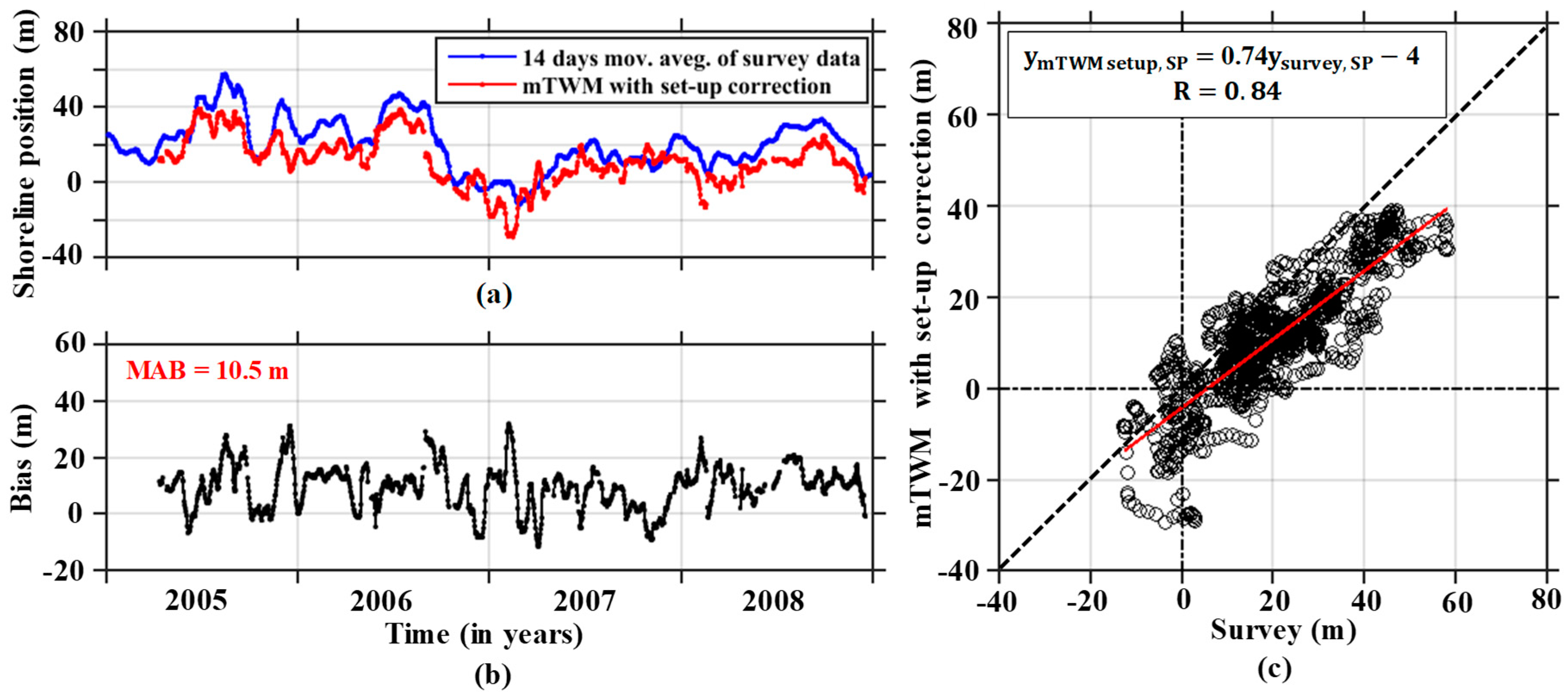
to compare the temporal updates of the extracted shoreline positions with corrected wave set-up and run-up with survey data.

2. Radar Observation and Data Processing

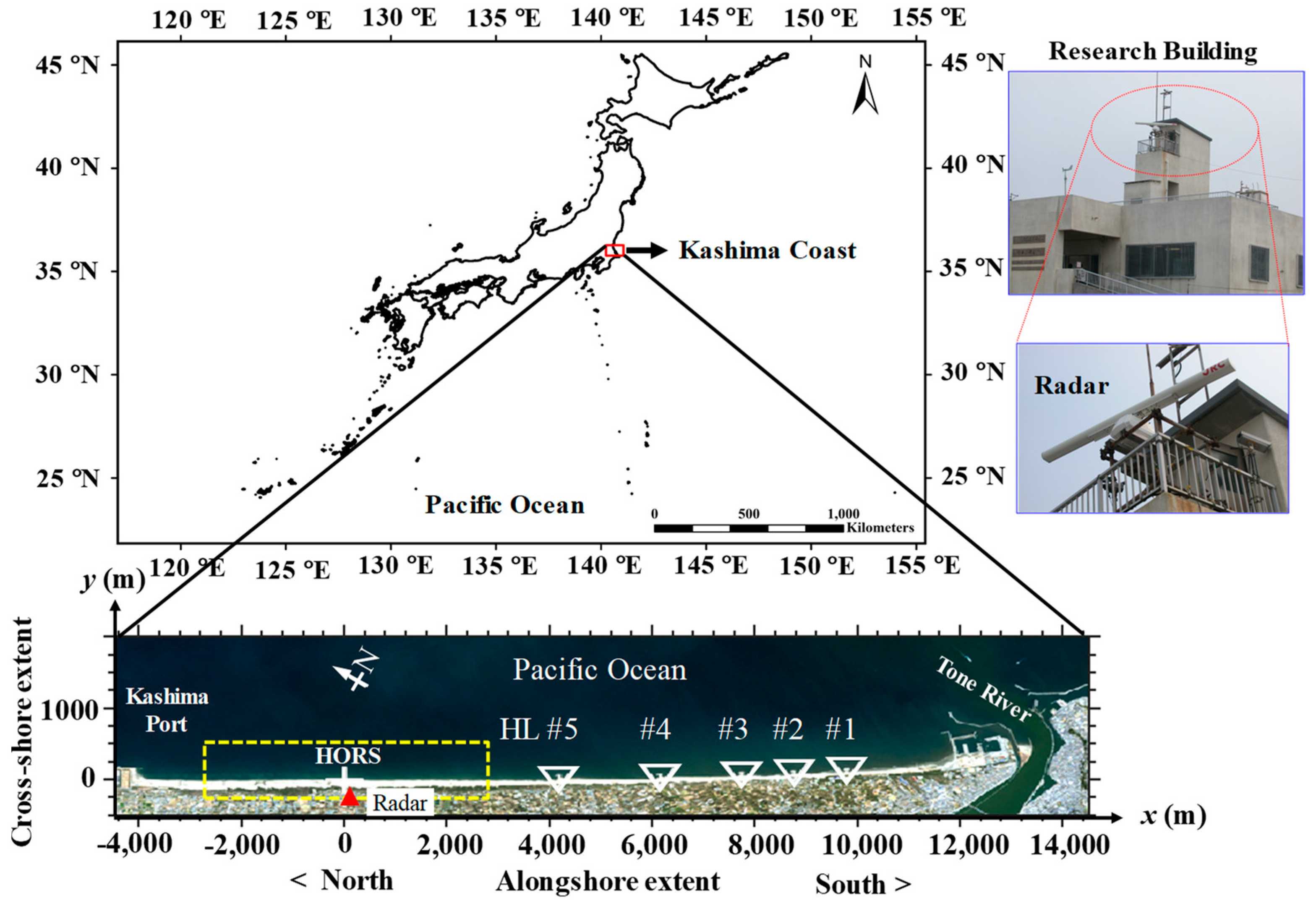
2.1. Study Site

The Kashima Coast, which is located in the Ibaraki Prefecture of Japan facing the South Pacific Ocean, is almost straight with a sandy beach that spread over an area spanning approximately 17 km. It is bounded on the south end by the Choshi Fishery Port and the north end by the Kashima Port. The study area is marked with the yellow rectangle box shown in Figure 1. The 400 m long field observation research pier is located in the center of HORS with the research building located on the backshore approximately 110 m backward from the mean shoreline position. The median sediment diameter is 0.18 mm and occasionally increases to 1.00 mm around troughs after severe storms [40]. Based on previous studies [41,42] at the single-bar Hasaki coast, the mean beach slope was 1/50, ranging from –60 to 200 m seaward and 1/200 in the deeper area.

2.2. Tide and Wave Data

The Japanese Meteorological Agency collects hourly tidal elevation data at Choshi Fishery Port, and the interannual variation is shown in Figure 2a. The tidal environment of this area is micro-tidal with a tidal variability range of approximately 1.5 m. Figure 2b–d show the variations in the significant wave height, period, and incidence angle, respectively. These data are measured every two hours at Kashima Port Station, where the mean water depth is approximately 24 m, as part of the Nationwide Ocean Wave Information Network for Ports and Harbors (NOWPHAS: http://nowphas.mlit.go.jp/eng.html).

2.3. X-Band Radar System and Time-Averaged Images

A conventional X-band radar measurement was conducted at HORS research pier of the Port and Airport Research Institute (PARI) in Hasaki, Japan. The 2.8 m radar antenna was mounted on the roof of the research building 17 m above mean sea level. The antenna rotated with a period of approximately 2.5 s and transmitted with a beam width of 0.8° in the horizontal direction and 25.0° in the vertical direction. The echo signals from the sea surface were grabbed with a specially designed A/D board installed on a computer, with sampling rate of 20 Mhz [6,43].

Individual echo images sampled every 2 s were averaged yielding a “time-averaged image” or so-called “time exposure” [6]. Ensembles of 512 individual echo images over 17 min (512 × 2 s = 1024 s) were processed to time-averaged radar images for every hour. Figure 3a shows an example of a time-averaged X-band radar image and coordinate system. The x-axis corresponds to the longshore extent, and the y-axis is taken in the cross-shore direction, positive toward the offshore. The echo signals are converted into a rectangular image size of 1024 pixels horizontal (longshore extent) and 512 pixels vertical (cross-shore extent). The pixel size of the rectangular image is approximately 5.42 m, whereas the theoretical spatial resolution of the radar system is approximately 7.5 m. Thus, the image covers an area spanning approximately 5556 m (1024 pixels) in the alongshore direction and 2778 m (512 pixels) in the cross-shore direction. The pixel intensities of the time-averaged gray images are belonging 0 (no backscatter) to 255 (saturation). Owing to reflections, individual waves disappear in the time-averaged radar images. A horizontal and bright edge extending in the longshore corresponds to the shoreline, which is marked in Figure 3a; the radar position is located at the center of the bottom edge in the figure, indicated by a black oval. The time-averaged images enable the identification of the intertidal bathymetry, breaker zone, rip current, bar crest locations, mega-cusp migrations, wave run-up, and other features [6,26,27,43,44,45]. Previously, Takewaka [6] examined the accuracy of the intertidal morphological feature using time-averaged images compared to field survey results. Hourly processed time-averaged images have been collected since 2005; however, some data gaps were reported due to mechanical trouble.

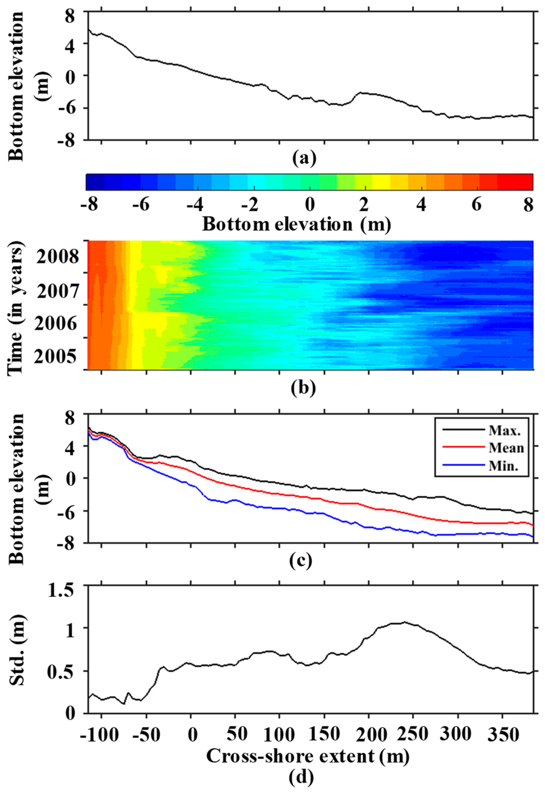
3. Beach Profile along the Pier

Beach profiles along the research pier were measured at 5 m intervals every day from −110 m to 385 m, except on weekends and national holidays. Figure 3b shows an aerial photo of the research pier. Figure 4a illustrates an example of a surveyed beach profile, and Figure 4b shows the variation in beach profile. Figure 4c displays the mean, maximum, and minimum beach profiles, whereas Figure 4d depicts their standard deviation. Small standard deviation values and narrow envelopes indicate stable regions, while large standard deviations and wide envelopes are associated with regions of high variability.

The shoreline position is defined where the bottom elevation is equal to 0.0 m (Tokyo Peil, T.P). The intertidal foreshore slope is defined as the linear slope of the beach profile ranging between the height of −0.8 m and 0.8 m. Figure 5a,b show variations in the shoreline positions and intertidal foreshore slopes during 2005–2008.

4. Shoreline Position and Intertidal Foreshore Slope Estimation

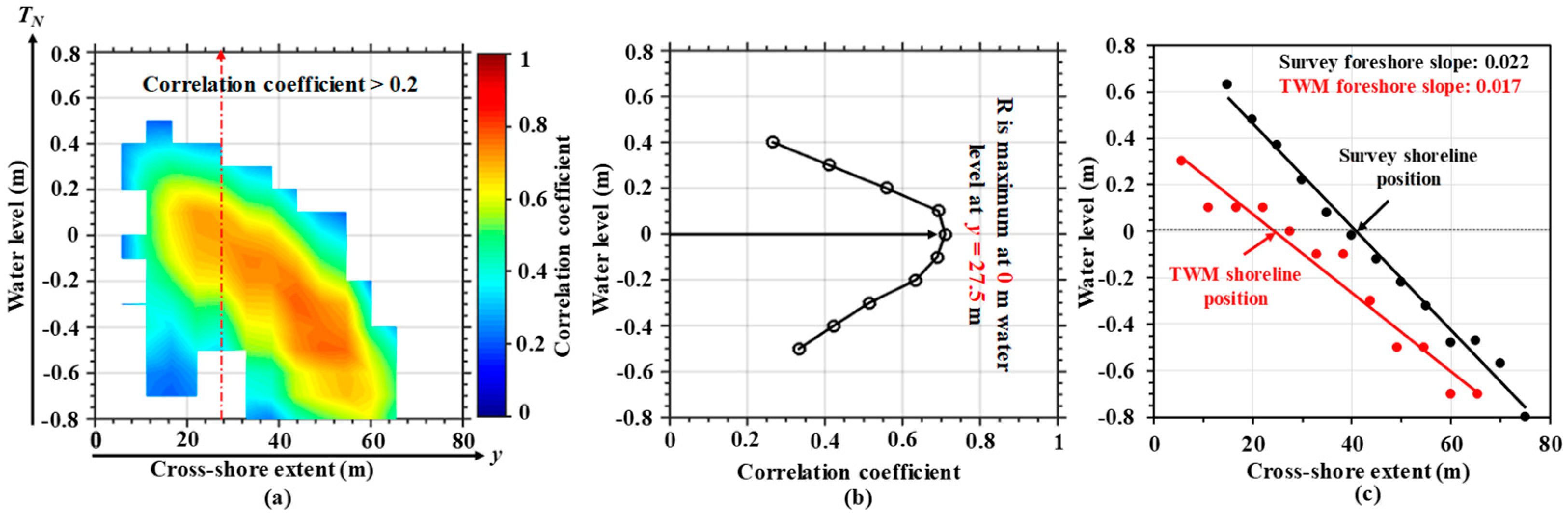
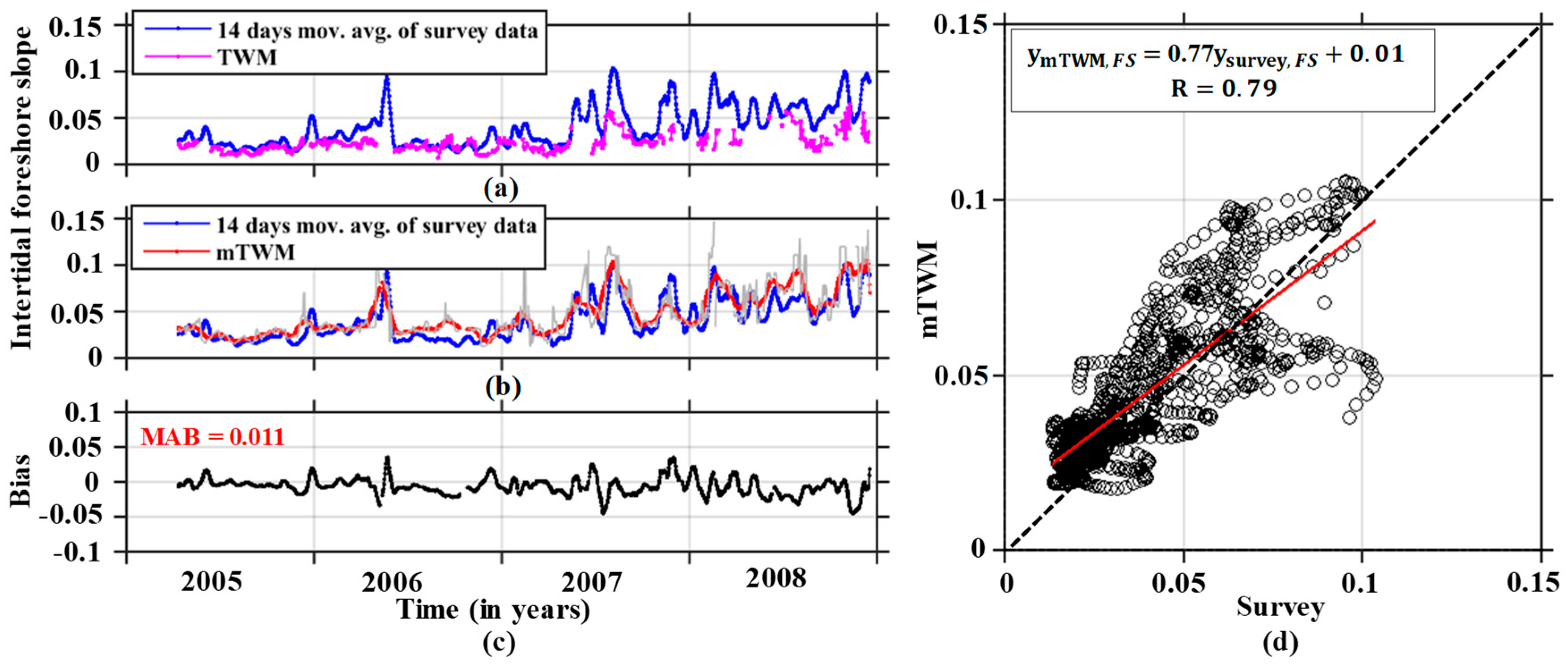
4.1. Intertidal Beach Profile and Shoreline Estimation Using TWM and mTWM

The TWM was developed by Bell et al. [28] to extract an intertidal beach profile from time-averaged X-band radar images considering the tidal variation, and the mTWM is the modified form of Bell et al.’s [28] approach. First, the basic concept of TWM and then our modification are described in this subsection.

Time-series of individual radar pixel intensities are gathered from hourly time-averaged images across the selected timescale of two weeks, including a full spring-neap cycle (as an example, June 17–30, 2005). Figure 6a displays the cross-shore time stack images within the range between $y=5$ m and $y=103$ m. The red line marked in Figure 6b indicates the variation of the instantaneous waterline position digitized manually by visual inspection, and Figure 6c is the concurrent tidal records. In general, the instantaneous waterline position is the boundary between the coastal land and water at one instant in every measurement. It can be clearly seen that the instantaneous waterline position moves seaward when the tide ebbs and vice versa (see Figure 6b,c).

At a longshore point $x$, the pixel intensity from the intertidal zone at $y$ is extracted from time-averaged images and repeated for two weeks, which yields $P \left(y,n\right)$ where $n$ is time. Figure 7a–d illustrate the variations in pixel intensities over a two weeks period, showing the periodic episode. High pixel intensities are acquired from time-averaged images when the waterline clearly appears, and vice versa.

The tidal elevation range between −0.8 and 0.8 m is considered with 0.1 m increments to generate binary pulse sequences, which are hereafter indicated with water level number $N$($N=-8,-7,\dots ,8$). The study site exhibits a micro-tidal influence with a tidal variability range of approximately 1.5 m. Each tidal elevation within a given tidal range of −0.8–0.8 m with 0.1 m increments has a unique binary pulse signal that representing 1 and 0, where 1 and 0 indicates a binary pulse sequence above and below water level at a given water level of the tidal cycle. Each elevation produced a unique binary pulse sequence, which is defined by $T_N\left(n\right)$, as illustrated in Figure 7e–g for $T_{N=-2}\left(-0.2 \mathrm{m}\right)$, $T_{N=0}\left(0 \mathrm{m}\right)$, and $T_{N=2}\left(0.2 \mathrm{m}\right)$, respectively. As shown in Figure 7, the extracted pixel intensities from time-averaged radar images and binary pulse signals at water levels have signal similarities.

Now, the correlation coefficient $R\left(y,N\right)$ is calculated at each possible elevation to measure the signal similarities between the pixel intensity variation $P\left(y,N\right)$ at different cross-shore extents, in addition to the tidal binary pulse sequence T_N(n) for different water level numbers:

$$R\left(y,N\right)=\frac{{\sum }_{n=1}^{24\times 14}\left\{\left(P\left(y,n\right)-\overline{P}\left(y\right)\right)\left(T_N\left(n\right)-{\overline{T}}_N\right)\right\}}{\sqrt{{\sum }_{n=1}^{24\times 14}{\left(P\left(y,n\right)-\overline{P}\left(y\right)\right)}^2} \sqrt{{\sum }_{n=1}^{24\times 14}{\left(\left(T_N\left(n\right)-{\overline{T}}_N\right)\right)}^2}}$$

(1)

where $\overline{P}\left(y\right)$ is the mean pixel intensity and ${\overline{T}}_N$ is the mean tidal binary pulse sequence over two weeks. A high correlation value indicates the strong signal similarities between the pixel intensity variation and binary representation of the tidal record sequence, which describes the implication for bottom elevation.

The tables at the right-hand side of Figure 7a–d illustrate the correlation coefficients between each tidal binary signal pulse (−0.2 m, 0 m and 0.2 m) with individual pixel intensity variation, and Figure 7e–g illustrate the correlation coefficient between the pixel intensity variation at $y=22$ m, $27.5$ m, $33$ m, and $38$ m with individual tidal binary signal pulses. The maximum correlation coefficient is used to indicate the cross-shore position at a certain water level, and the process is repeated for all binary signal tidal elevation extracted from tide records. The outcomes are then utilized to plot a correlation map for a given longshore extent ($x=-49$ m) at different water levels (−0.8 to 0.8 m with 0.1 m increments) within the intertidal range ($y=0–80$ m with 5.4 m increments), as shown in Figure 8. Here, no correlation coefficients are available at water levels of 0.6–0.8 m because the correlation values less than 0.2 at the 0.6 m level and the tide level did not reach 0.7 m and 0.8 m levels.

By using the correlation coefficient map in Figure 8, the intertidal shore profile can be determined in the following two ways:

(i) To detect the water level from a cross-shore position correlation coefficient distribution, where the distribution is maximum. The detected point is regarded as the bottom elevation. Similarly, the maximum correlation at other water levels are estimated throughout the remaining cross-shore positions, and the intertidal cross-shore profile is determined. This approach is known as TWM, which was initially introduced by Bell et al. [28].

(ii) To detect the cross-shore position from the distribution of correlation coefficients across a water level, where the distribution is maximum. The detected point is also regarded as the bottom elevation. Proceeding the same way, the maximum correlation is established at other cross-shore positions across the remaining water levels, and the intertidal cross-shore profile is produced. This approach is called mTWM, which is the modified form of Bell et al.’s [28] approach.

Figure 9a shows an example of the correlation map for a given longshore extent ($x=-49$ m) at different water levels (−0.8–0.8 m with 0.1 m increments) within the cross-shore extent (y = 0–80 m with 5.4 m increments). The red arrow line indicates an example of the cross-shore position transect at $y=27.5$ m. Figure 9b shows the correlation coefficient distribution at $y=27.5$ m extracted from the map within the water levels range (−0.5–0.4 m). The maximum correlation is established at 0.0 m water level, which is regarded as the bottom elevation of this point. Similarly, the maximum correlation at other water levels are determined among the remaining cross-shore positions, and the intertidal cross-shore profile is estimated. Then, a linear fitting model is applied to determine the shoreline position at 0.0 m water level, and the intertidal foreshore slope is calculated from regression line coefficient within the intertidal range. As shown in Figure 9c, the shoreline position is determined at $y=24.3$ m, and the intertidal foreshore slope is 0.017. Compared to the surveyed shore profile, we observed that the TWM failed to estimate the shore profile accurately from radar images.

In TWM, to look for water levels from the distribution of correlation coefficients along the cross-shore positions, the maximum correlation coefficient is frequently established between −0.8 m and 0.4 m water levels. Due to the strong similarities between the cross-shore position pixel intensities extracted from images and tidal binary pulse signals (−0.8 to 0.4 m), a high correlation coefficient frequently appears at these water levels. In another sense, the original TWM cannot detect the water levels (0.5–0.8 m) due to the presence of lower correlation coefficients than in other water levels (−0.8 to 0.4 m). As a result, the TWM failed to estimate the actual intertidal shore profile and was unable to determine the shoreline position and intertidal foreshore slope with a significant bias.

Landwards cross-shore position pixel intensities have no periodic oscillation like tidal binary pulse signals, which is due to the irregularity of water line with time for each transition. In such reason, cross-shore position pixel intensities and tidal binary pulse signals provide poor and almost identical correlation coefficient values. Therefore, cross-shore direction-wise water level detection technique (TWM) is failed to estimate the expected objects. Under a changed search direction (mTWM) to find the bottom elevation, the extracted intertidal shore profile becomes closer to the survey profile. The above-described bottom elevation finding approach is considered as the modification in this study. Prior to estimating the intertidal shore profile, the input of the intertidal range was selected from the tidal elevation data. To ensure each of water levels in the intertidal shore profile, it is expected that the water level wise cross-shore position detection is more appropriate than TWM. The performance of this approach will be described later.

Figure 10a displays a correlation map for a given longshore extent ($x=-49$ m) at different water levels (−0.8–0.8 m with 0.1 m increments) within the intertidal range ($y=0–80$ m with 5.4 m increments). The red arrow line indicates an example of a 0.0 m water level transect. Figure 10b shows the correlation coefficient distribution at a water level of 0.0 m extracted from the map within the cross-shore extent range ($0\le y\le 80$ m). The maximum correlation is established at the $y=27.5$ m cross-shore position, which is regarded as the bottom elevation of this point. Similarly, the maximum correlation at other cross-shore positions are determined among the remaining water levels and the intertidal cross-shore profile is estimated. Then, a linear fitting model is applied to determine the shoreline position at the 0.0 m water level, and the intertidal foreshore slope is calculated from regression line coefficients within the intertidal range. The shoreline position in Figure 10c is determined at $y=30$ m, and the intertidal foreshore slope is 0.024. We compared the estimated slope with a survey intertidal profile slope on 17 June 2006. Figure 10c shows that the mTWM estimated intertidal foreshore slope is very close to the survey slope; however, the extracted shoreline positions have some landward shifts compared to the survey data. This shift is induced by the effect of wave set-up or wave run-up. The correlation coefficients greater than 0.2 is used for the both cases.

The data collected over a two-week period were processed to obtain shoreline position and intertidal foreshore slope data. This process was repeated between 12 April 2005 and 31 December 2008 to estimate variations in the shoreline position and intertidal foreshore slope. Figure 11a,b depict variations in the shoreline position derived by TWM and mTWM compared to those obtained by survey data collected at the research pier; however, some random gaps are observed owing to the lack of strong waterline signals or the saturation of echo signals. The bias between the results obtained by survey data and mTWM derived results is presented in Figure 11c, showing 14 m mean absolute bias (MAB). A similar trend is observed between the shoreline positions estimated by mTWM and the survey data, which is confirmed by the correlation coefficient ($R=0.86$), shown in Figure 11d; however, a horizontal shift is detected between the mTWM derived results and surveyed shoreline positions. This shift is induced by the effect of wave set-up or wave run-up or by a combination of correction factors and will be discussed in Section 4.2 and Section 4.3. On the other hand, the calculated MAB between survey and TWM derived shoreline positions is 19.2 m, which is larger than the obtained MAB between survey and mTWM. The large number of random gaps also appear in the TWM estimation and are effects of linear regression conditions. This is clearly visible in Figure 11a.

Figure 12a,b present the temporal variations in intertidal foreshore slopes derived by TWM and mTWM during the study period and present the survey data, and the bias between those obtained from the survey and mTWM outcomes are shown in Figure 12c. Compared to the surveyed slopes, TWM-estimated slopes are approximately three times milder. That means TWM cannot estimate the slopes accurately from radar images. The reason for this discrepancy is described above. In order to estimate the bias, the radar-detected values at each time point were subtracted from the survey detected values. The surveyed slope is sometimes steeper than that estimated by the mTWM owing to the comparison between different cross section transect estimated observations. This discrepancy can be attributed to the fact that survey data are collected along the research pier, while data used for the mTWM are extracted 49 m far from the research pier. In addition, a fixed gap is observed along the research pier $(-49<x<65$ m) due to saturated echo signals.

Water flows typically faster around piers and abutments, making them susceptible to local scour or the removal of sediment [46]. Due to local scour, sand is eroded around the pier and accumulated to the near side. As a consequence, the cross-shore beach profile changes gradually along the pier, and beach slopes can be steeper than the surroundings. Authors have visited the study site several times and sometimes found steeper foreshore close to the pier. This may be one possible reason for the discrepancy in intertidal foreshore slope estimations.

The mTWM is applied to all alongshore locations; the spatiotemporal variations in the shoreline positions and intertidal foreshore slopes for the entire area are obtained for the period between 12 April 2005 and 31 December 2008, as shown in Figure 13. The x-axis denotes alongshore extent, and the y-axis denotes the time history between 2005 and 2008. The color bar of Figure 13a indicates the landward (blue) and seaward (red) shoreline positions from its origin. On the other hand, the color bar pattern of Figure 13b shows the milder (blue) and steeper (red) intertidal beach slopes. However, 3% of the estimates are missing owing to the previously mentioned reason.

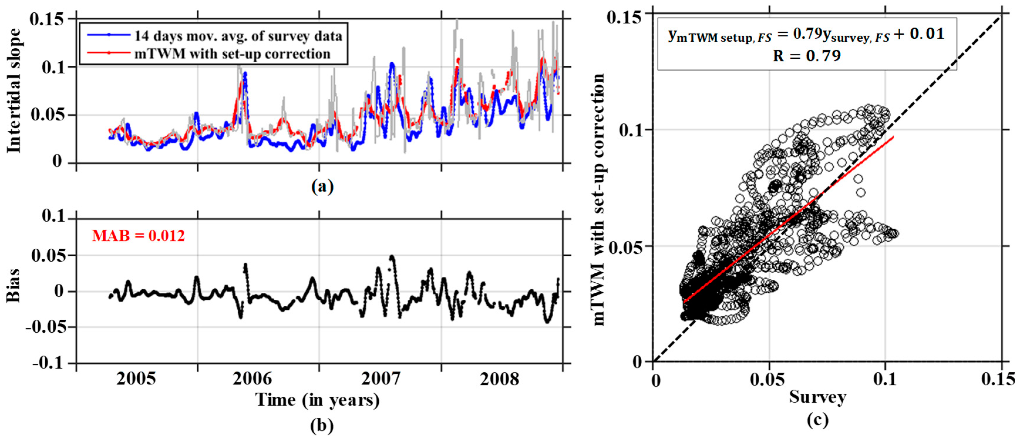
4.2. Wave Set-up Correction

Wave set-up is defined as an increase in the mean water level above the still water level owing to momentum transfer to the water column with the presence of breaking waves, which is a common dynamic process in the nearshore zone [47]. Within the surf zone where wave breaking dissipates energy, the wave thrust decreases as the breaking surge travels shoreward; consequently, the mean water level rises, and thus wave set-up occurs. Figure 14a is a schematic illustration of the wave set-up that indicates the corresponding rise in waterline. It shows that the mTWM estimated results are shifted landwards compared to the survey data. Hence, the correction of wave set-up on the mTWM is essential to reduce the horizontal shift in shoreline positions. Based on this schematic scenario, the following strategy is adopted to correct the wave set-up and to obtain more accurate results by mTWM.

Several studies have been conducted on the wave set-up on sloping beaches. In this study, the following empirical formula is used to estimate the amount of wave set-up ($\eta$) at Hasaki beach caused by normal wave incidence [48]:

$$\frac{\eta }{H_0}=A_0+A_{1}log\left(H_0/L_0\right)+A_2{\left(log\left(H_0/L_0\right)\right)}^2$$

(2)

and

$$\begin{array}{c}{A}_0=0.0063+0.768 tan\beta \\ A_1=-0.0083-0.011 tan\beta \\ A_2=0.00372+0.0148 tan\beta \end{array}\}$$

(3)

where $tan\beta$ is the bottom slope; $H_0$ is the offshore wave height, which is determined by the linear wave theory equation $H_1=H_0{K}_r{K}_s$ where $K_r$ is the refraction coefficient, $K_s$ is the shoaling coefficient, and $H_1$ is the NOWPHAS wave height; and $L_0$ is the offshore wave length, which is determined by $L_0=1.56T^2$ and where $T$ is the wave period.

The amount of wave set-up $\mathsf{\Delta }\eta$ at Hasaki beach due to oblique wave incidence is given by [48]

$$\mathsf{\Delta }\eta =\eta \times {\left(cos{\theta }_0\right)}^{0.545+0.038 log\left(H_0/L_0\right)}$$

(4)

where, ${\theta }_0$ is the offshore wave direction estimated by Snell’s law.

The amount of wave set-up is calculated for every two-hour time frame using Equations (2)–(4), as shown in Figure 15. In order to determine the wave set-up, the mean beach slope (0.04) is used, which is extracted by the mTWM from radar images during 2005–2008. A set-up corrected water level for the mTWM estimates is set by adding the wave set-up to the tide record, as shown in Figure 16. The corrected water level is shifted upward by approximately 0.17 m compared to the original tide record. A new correlation map is established with the corrected water level at $x=-49$ m shown in Figure 17a. The correlation coefficients obtained at the 0.0 m water level at cross-shore positions ($0\le y\le 80 \mathrm{m}$) are shown in Figure 17b with solid red circles. The maximum correlation is now established at $y=33$ m. Similarly, the obtained intertidal beach profile with corrected tide signal is shown in Figure 17c. The results of the linear regression analysis indicate the estimated shoreline position at $y=34$ m with intertidal foreshore slope $\beta =0.024$. The shoreline position is now shifted 4 m landwards, while the intertidal foreshore remains almost the same. Hence, it may be expected that we can apply the tidal variation-based intertidal foreshore slopes extracted by mTWM for further analysis.

Figure 18a depicts a comparison between the survey and mTWM-extracted shoreline positions with corrected set-up, and the vertical elevation bias between the survey and mTWM results with a corrected wave set-up is shown in Figure 18b. As shown in Figure 18c, the correlation coefficient ($R=0.84$) in both cases is almost equivalent to the previously obtained results. Similar trends are observed between shoreline positions obtained by the mTWM with a corrected wave set-up and the survey data; however, the MAB of the estimated results dropped from 14 m to 10.5 m.

The variation in intertidal foreshore slope with a corrected wave set-up that shown in Figure 19 is similar to the previously estimated results (Figure 12).

Figure 18 and Figure 19 confirm the effectiveness of the corrected wave set-up to determine the shoreline positions using the mTWM accurately. It allows shifting of the estimated shoreline position landward without changing the shape of the intertidal beach profile.

The mTWM with a corrected wave set-up is applied to all alongshore locations; the spatiotemporal variations in shoreline positions and intertidal foreshore slopes can be obtained for the entire study site from 12 April 2005 to 31 December 2008. For the sake of simplicity, wave set-up corrected spatiotemporal variations in shoreline positions and intertidal foreshore slopes are not shown in the manuscript.

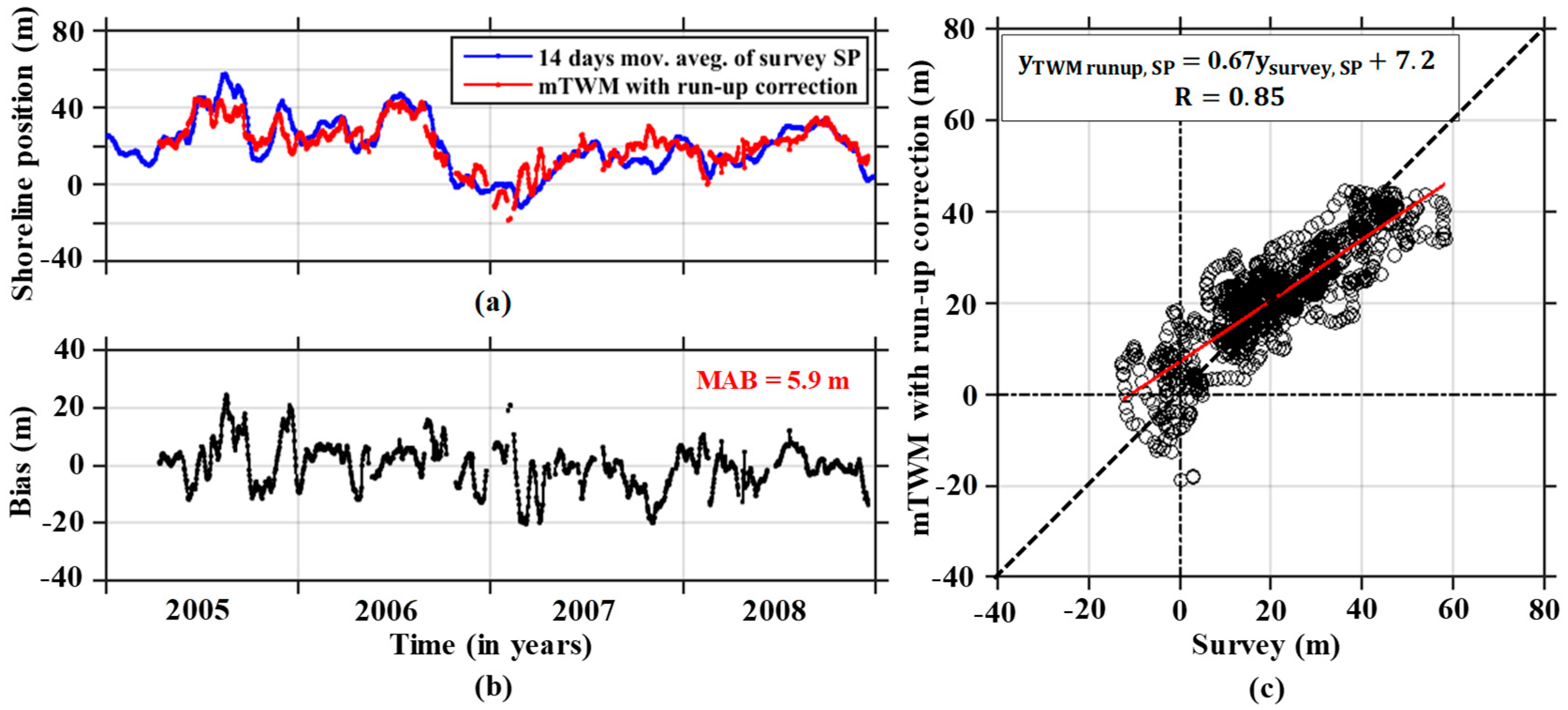
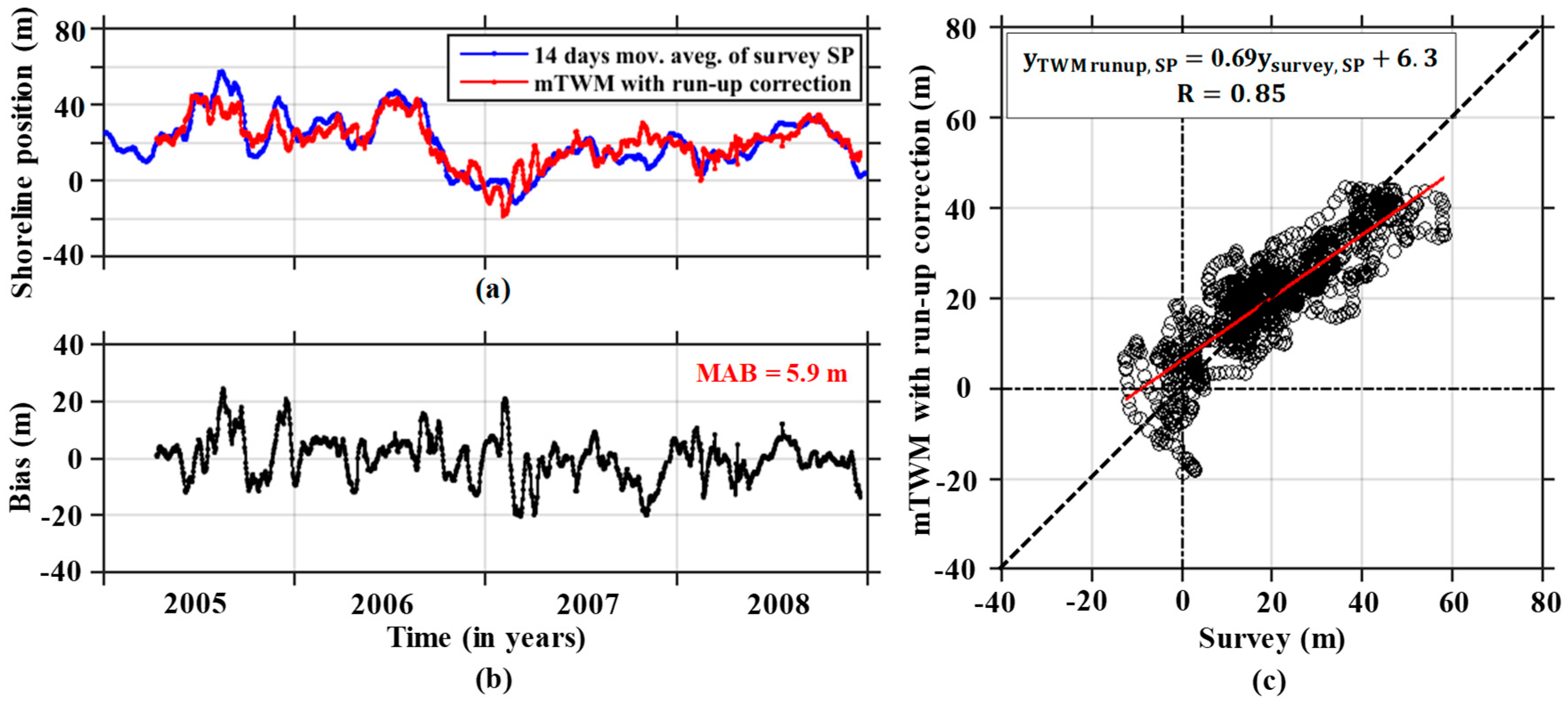
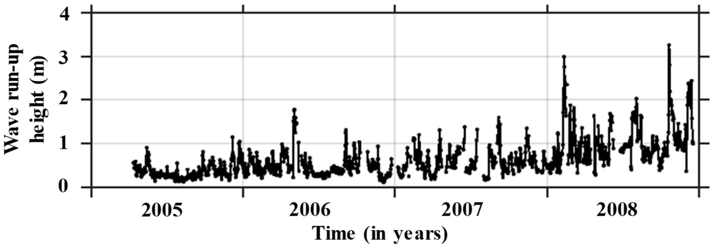
4.3. Wave Run-up Correction

Wave run-up is defined as “the landward extent of wave uprush measured vertically from the still water level” [49]. Accordingly, during high wave conditions, the waterline positions shift more landward owing to the wave run-up effect. Basically, the run-up characteristics change with the beach slope and offshore wave properties. Figure 14b is a schematic illustration showing that the results obtained by the mTWM extraction with a corrected wave run-up are further shifted landward compared to the survey data. Hence, it may expect that the corrected wave run-up is essential to accurately determine the shoreline positions for the study site. The following strategy is adopted to correct the wave run-up to obtain more accurate estimates by the mTWM:

Based on both field and laboratory observations, Hunt [50] initially proposed the following wave run-up formula, which is typically defined by

$$\frac{R}{H_0}=c{\xi }_0+d$$

(5)

where R is the vertical run-up normalized by the offshore wave height H₀ and c and d are dimensionless constants.

Several researchers [51,52,53,54,55] have investigated the amount of wave run-up on intermediate to reactive beaches by using video camera analysis. Hasan and Takewaka [44] first analyzed wave run-up using data extracted from X-band radar images at Hasaki beach and established a formula to calculate the infragravity wave run-up:

$$\frac{R}{H_0}=1.025{\xi }_0+0.03$$

(6)

where ξ₀ is the surf similarity parameter [56] and is expressed by

$${\xi }_0=\frac{tan\beta }{\sqrt{H_0/L_0}}$$

(7)

where $tan\beta$ is the beach slope, $L_0$ is the deep-water wave length defined as $L_0=g{T}^2/2\pi$, $g$ is the gravitational acceleration, and $T$ is the wave period. The low surf similarity parameters (${\xi }_0\le 0.3$) usually specify a dissipative beach condition while higher values suggest a more reactive condition. Figure 20 shows the variation in wave run-up height along a transect at $x=-49$ m over the period 12 April 2005 to 31 December 2008 using Equations (6) and (7). $H_0$ and $L_0$ are calculated from the wave records, and the intertidal foreshore slope ($tan\beta$) is derived from mTWM estimation considering tidal variation.

The following formula is employed to correct the wave run-up effect on the shoreline position derived by the mTWM:

$$mTWM runup corrected SP=mTWM estimated SP+\left(\frac{Wave runup height}{mTWM estimated slope}\right)$$

(8)

where the second term on the right side denotes the landward horizontal shift due to wave run-up, which is known as the wave run-up length, and the 14-day moving average filter is used for the wave run-up length calculation.

The variations in shoreline position obtained by the mTWM with corrected wave run-up compared to the survey data are illustrated in Figure 21a. Correspondingly, the vertical elevation bias between the survey and mTWM-estimated results with corrected wave run-up is shown in Figure 21b, and the MAB is further reduced to 5.9 m (compared to the original value of 14 m), which is theoretically smaller than the spatial resolution of the radar measurements described in Section 2.3. The correlation coefficient between the shoreline position obtained by the mTWM with corrected wave run-up and survey data is 0.85, as shown in Figure 21c, which is almost equivalent to the previously estimated results. The results show that the utilized method can successfully estimate the shoreline position from radar images after corrected wave run-up.

The mTWM with corrected wave run-up is applied to all alongshore locations to determine the spatio-temporal variation in shoreline positions for the entire study area over the period between April 12, 2005 and December 31, 2008, as shown in Figure 22.

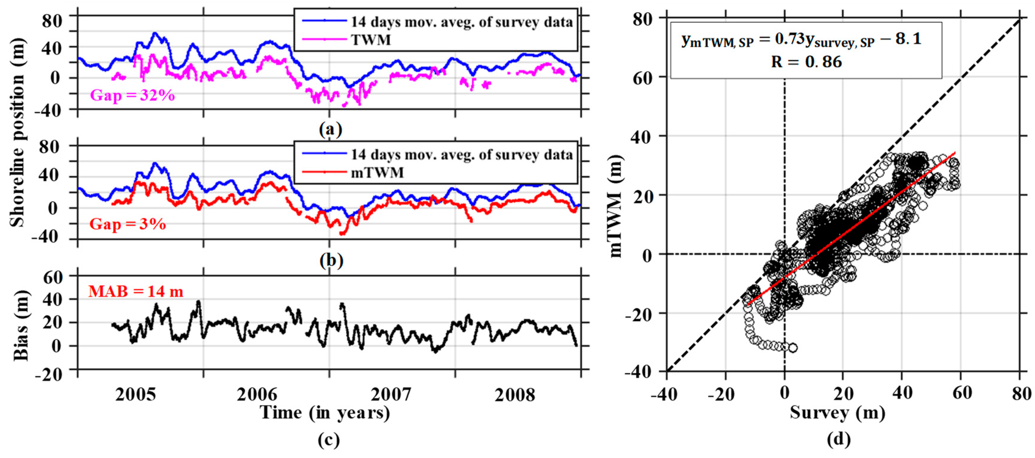
4.4. Shoreline Position Data Gaps Filled by Garcia’s Method

The white blanks in Figure 22 indicate the 3% gaps in the shoreline data derived by mTWM owing to the lack of strong waterline signals caused by overflooding, the existence of strong radar reflectors, etc. Garcia’s smoothing and gap filling method [57] was employed to fill these gaps, and the validity of this method will be checked.

Garcia’s method is formulated based on a Penalized Least Squares regression by means of the Discrete Cosine Transform (PLS-DCT), which expresses the data in terms of a sum of cosine functions oscillating at different frequencies and is suitable for equally spaced data in one dimension and higher. As the DCT can be multidimensional, the DCT-based PLS regression can be instantly extended to multidimensional datasets. Furthermore, this method was adopted by Wang et al. [58], and its performances to fill the gaps in a global soil moisture dataset was analyzed. Recently, Bell et al. [28] and Bird et al. [29] have employed this algorithm to fill the gaps in beach profile data. This method will be adopted in this study to fill the random gaps in the temporal or spatiotemporal shoreline datasets.

To evaluate the performance of Garcia’s method, the numerous random gaps in the mTWM derived shoreline positions with corrected wave run-up are considered. Figure 23a depicts the temporal variation in gap-filled shoreline positions with corrected wave run-up. The gaps in shoreline positions are filled by Garcia’s method. The bias distribution between the survey data and mTWM extracted shoreline position results with corrected wave run-up is shown in Figure 23b with a MAB of 5.9 m, which is equivalent to that obtained before applying Garcia’s method. As shown in Figure 23c, the gap-filled result implies that the variations in shoreline position are synchronized, which is confirmed by the good correlation coefficient (R = 0.85). This value is almost equivalent to that obtained before applying Garcia’s method on the wave run-up correction shoreline positions. Therefore, the estimated variation of shoreline positions with corrected wave run-up are quite similar to the survey data. The efficiency of Garcia’s filling method will be explained in the discussion section.

Based on the above results, Garcia’s method is implemented to fill the gaps in the entire spatiotemporal shoreline position data derived by mTWM with corrected wave run-up (Figure 22). Figure 24a shows the gap-filled spatiotemporal distribution of wave run-up corrected shoreline positions extracted from time-averaged X-band radar images over four years (2005–2008). The rainbow patterns of the color bar indicate the landwards (blue) and seawards (red) positions of shoreline from its origin. Correspondingly, Figure 24b,c show the spatial mean of the shoreline positions and temporal variations in significant wave height, respectively. The adopted gap-filling method demonstrates a reasonably good performance in terms of the smoothness of the shoreline data. Figure 24 suggests that Garcia’s method is capable of filling the numerous random gaps in the shoreline position data. Moreover, we may conclude that Garcia’s method combined with mTWM performs reasonably well to fill the random gaps in the shoreline position data, generating results nearly similar to the survey data. The results show seaward shifts of shoreline positions due to low wave conditions and landward shifts due to high wave conditions. The obtained result is in good agreement with Galal and Takewaka’s [59] reported outcome. The obtained features were initially reported by Kuriyama and Lee [60] and is called beach cycle. Huge erosion was observed in October 2006, which was a result of high waves and storm surge attacking the Kashima Coast. Based on the results obtained by mTWM, we can be assured that the mTWM is a robust approach to detect intertidal shore profiles automatically from time-averaged X-band radar images, and it can be used any beach in the world to help the authorities to understand long- or short-term shoreline changes in coastal zones.

5. Discussion

This section discusses the mTWM extracted results, its adopted correction, and the possible reasons for the large bias. The purpose of this study was to automatically detect the shoreline positions and intertidal foreshore slopes using the mTWM. The automatic extraction of shoreline positions and intertidal foreshore slopes has been successfully performed, but systematic biases in the shoreline positions have been observed. The shoreline position estimated by the mTWM shifted landward, with a MAB of 14 m.

Similar shifts in estimated shoreline positions were reported in previous studies [6,28]. Takewaka [6] initially analyzed the time-averaged X-band radar images at Hasaki beach, Japan to estimate the shoreline positions and intertidal foreshore slopes by manual inspection. In this study, the horizontal shift between the estimated and surveyed shoreline positions was measured as 10 m. Recently, Bell et al. [28] automatically acquired intertidal shore profile datasets for Hilbre Island at the mouth of Dee Estuary, UK. To validate the accuracy of the calculated results, they compared the TWM-generated results with airborne LIDAR surveyed data for the same study site over the radar survey period. The vertical elevation bias between the two intertidal shore profiles is approximately ±0.5 m. This can lead to horizontal shifts in the estimated shoreline positions depending on the beach slopes and wave conditions. If the beach slopes (1:20–1:100) vary with high wave conditions, the horizontal shift between the two observations can also vary (10–50 m). In both studies, the effects of wave set-up and run-up on reducing the horizontal shift were not considered.

The schematic illustration in Figure 14 suggests that wave set-up and run-up may be causing this type of horizontal shifts. Two correction methods were tested to reduce such systematic bias. The correction of wave set-up evaluates a mean waterline above a still water level and allows a horizontal distance between such waterline and tidal level [10]. Figure 18b shows the distribution of the bias between the survey data and shoreline positions derived by mTWM with corrected wave set-up. The MAB dropped by 3.5 m compared to the results obtained before applying a wave set-up correction to the shoreline position derived by mTWM (from 14 to 10.5 m); however, horizontal shifts were still present. This may suggest that Equations (2)–(4) are used appropriately to reduce some of the detected horizontal shifts in the study site; however, it was not bound in the spatial resolution of radar measurement.

To further reduce the horizontal shifts in the estimated shoreline positions and intertidal beach slopes, a wave run-up empirical formula is applied to achieve an upward shift of waterline position as well as a horizontal shift to the landward direction. The bias distribution between the survey and shoreline positions with corrected wave run-up is shown in Figure 21b, with a MAB of 5.9 m, which is smaller than the theoretical resolution of the radar measurements described earlier and the horizontal shift of bias that obtained by Takewaka [6]. Considering the use of X-radar images with a theoretical resolution of 7.5 m/pixel, the obtained MAB of 5.9 m is acceptable for an automatic application. Sometimes, the bias of estimated shoreline positions is higher than the spatial resolution of the radar measurements.

Figure 25a shows the frequency distribution of the estimated bias of shoreline positions. The estimated bias is the difference between the survey and mTWM-extracted run-up corrected gap-filled shoreline positions for each measurement. The distribution of the bias seems to follow the normal distribution, with a mean value of −0.05 m and a variance of 5.9 m. Hence, the overall results indicate that about 84% of the bias of the estimated shoreline positions are limited in the spatial resolution of the radar measurement and that the rest are slightly higher than the spatial resolution. The reason for the significant bias of the estimated shoreline positions will be described below. On the other hand, Figure 25b displays the frequency distribution of the estimated bias between the survey and only Garcia’s method gap-filled shoreline positions. This estimated bias of shoreline positions is bound in [−10 m, 10 m]. That means Garcia’s method interpolates nearly similar shoreline positions like the mTWM-derived shoreline positions. As shown in Figure 25b, the distribution of the bias seems to follow the normal distribution, with a mean value of −0.1 m and a variance of 3 m, where the 32 data are used in this case.

Figure 26a shows the scatter plot between the mTWM-estimated intertidal slope and the estimated bias of the shoreline positions. It seems that the bias become large when the mTWM-estimated intertidal foreshore slopes are in the milder range (0.01–0.06). In such a beach slope condition, the waterline position easily shifted landward and the shoreline position also moved landward. As a result, it sometimes surpasses the survey shoreline position and produces negative shoreline bias. On the contrary, sometimes it falls behind the survey shoreline position for the same beach slope condition and produces a positive shoreline bias. The milder beach slope is not the only reason for this bias; it also depends on wave action. It is noteworthy that the estimated bias is still within the acceptable limits for steeper beach slope conditions (0.06–0.1). In such conditions, the shoreline position cannot be moved easily in a landward direction without an extreme weather event such as a typhoon. As shown in Figure 26b, these features are verified by the relationship between the frequency distribution of slopes with 0.1 equal intervals and the corresponding estimated MAB of shoreline positions. It is also seen in Figure 26b that the high frequency of a milder slope produces the large MAB of shoreline positions. As mentioned before, the action of waves (low and high) might also play an influential role in significant bias. The cumulative frequencies indicate the 75% milder slopes (0.01–0.06) can follow the abovementioned characteristics.

Figure 27a shows the relationship between the 14-days moving averaged wave height and the estimated bias of shoreline positions. It is remarkable to observe that the bias of shoreline positions (positive or negative) becomes large when the waves are in low or high conditions with same beach slope. These features are confirmed in Figure 27b by the relationship between the frequency distribution of a wave height with 0.5 m equal intervals and the corresponding estimated MAB of shoreline positions. It can also be seen that the action of high waves produces significant MABs of the shoreline positions and vice versa. The cumulative frequencies indicate that 90% of waves can follow the abovementioned characteristics. Overall, the obtained results also show that the intertidal foreshore slopes (steeper or milder) and waves (low or high) are influential parameters for shoreline bias (positive or negative). It is further noted that some significant bias is also to be expected due to the different cross-sectional transect comparison of radar and survey-derived data.

Based on the results obtained by the gap-filled corrected wave run-up, we may conclude that more accurate shoreline positions are derived by mTWM with corrected wave run-up, which is very close to the survey data. This confirms that the correction of wave run-up and the application of Garcia’s method are the most reasonable strategies to reduce horizontal shifts in shoreline positions at Hasaki beach, Japan.

6. Conclusions

The mTWM is presented as a way to detect shoreline positions and intertidal foreshore slopes from X-band radar images. The method is slightly modified from the Bell et al. [28] approach (TWM). Cross-shore direction-wise bottom elevation estimation was considered as the TWM. Due to the presence of low signal similarities between pixel intensities and tidal binary signals at the landward cross-shore location, the TWM failed to estimate an accurate intertidal shore profile. Hence, determining the water level direction-wise bottom elevation and detecting intertidal shoreline profile are considered as the mTWM. The mTWM is successfully employed to detect accurate shoreline positions and intertidal foreshore slopes from X-band radar images collected over the course of two-week tidal cycle variation at microtidal sandy Hasaki beach, Japan, during 12 April 2005 to 31 December 2008. Compared to the survey data, the MAB of the detected shoreline positions was 14 m.

To reduce the horizontal shift between the shoreline positions derived by mTWM and the survey data, the corrected wave set-up was applied to the tidal record to compensate for the shift in the estimated results. The MAB between shoreline positions derived by mTWM with corrected wave set-up and the survey data was reduced to 10.5 m. Furthermore, the correction of the wave run-up was applied to the results obtained by the mTWM. This reduced the MAB to 5.9 m, which is smaller than the theoretical spatial resolution of X-band radar images; however, sometimes the estimated bias was larger than the spatial resolution. This larger bias is the effect of milder intertidal foreshore slopes and the action of waves. The frequency distribution results indicate that 84% of the estimated bias of the shoreline positions is limited in the spatial resolution of the radar measurement. On the other hand, numerous random gaps still existed in the dataset. These random gaps are due to a lack of strong waterline signals caused by overflooding, the existence of strong radar reflectors, etc.

To fill the random gaps, Garcia’s method was applied in the mTWM-derived shoreline positions with the corrected wave run-up. The MAB between these estimated shoreline positions and the survey data was 5.9 m, and the frequency distribution of the estimated bias of shoreline positions was 84%, which are almost equivalent to that obtained before applying the gap-filling method. On the other hand, the bias between the survey and only Garcia’s method filling shoreline positions are limited with [−10 m, 10 m]. This indicates the reliability of Garcia’s method. We can conclude that the mTWM integrated with this method is an efficient and robust approach to automatically detect shoreline positions from time-averaged X-band radar images with the consideration of a wave run-up correction at sandy beaches during various periods and to demonstrate the practicability of the utilized method. Therefore, the temporal and spatial variations of a shoreline can be automatically and continuously monitored over the long term to help authorities understand coastal changes, facilitating coastal protection and sustainable development in coastal zones.

References

1. Dolan, R.; Hayden, B.P.; May, P.; May, S. The reliability of shoreline changes measurements from aerial photographs. Shore Beach 1980, 48, 22–29. [Google Scholar]
2. Boak, E.H.; Turner, I.L. Shoreline definition and detection: a review. J. Coast. Res. 2005, 21, 688–703. [Google Scholar] [CrossRef]
3. Crowell, M.; Leatherman, S.P.; Buckley, M.K. Historical shoreline change: Error analysis and mapping accuracy. J. Coast. Res. 1991, 7, 839–852. [Google Scholar]
4. Camfield, F.E.; Morang, A. Defining and interpreting shoreline change. Ocean Coast. Manag. 1996, 32, 129–151. [Google Scholar] [CrossRef]
5. Kraus, N.C.; Rosati, J.D. Interpretation of Shoreline-Position Data for Coastal Engineering Analysis; Coastal Engineering Technical Note II-39 (No. CERC-CETN-II-39); U.S. Army Engineer Research and Development Center: Vicksburg, MS, USA, 1997. [Google Scholar]
6. Takewaka, S. Measurements of shoreline positions and intertidal foreshore slopes with X-band marine radar system. Coast. Eng. J. 2005, 47, 91–107. [Google Scholar] [CrossRef]
7. Hanslow, D.J. Beach erosion trend measurement: a comparison of trend indicators. J. Coast. Res. 2007, 50, 588–593. [Google Scholar]
8. Ryu, J.H.; Kim, C.H.; Lee, Y.K.; Won, J.S.; Chun, S.S.; Lee, S. Detecting the intertidal morphologic change using satellite data. Estuar. Coast. Shelf Sci. 2008, 78, 623–632. [Google Scholar] [CrossRef]
9. Chen, W.W.; Chang, H.K. Estimation of shoreline position and change from satellite images considering tidal variation. Estuar. Coast. Shelf Sci. 2009, 84, 54–60. [Google Scholar] [CrossRef]
10. Chang, H.K.; Chen, W.W.; Liou, J.C. Shifting the waterlines of satellite images to the mean water shorelines considering wave runup, setup, and tidal variation. J. Appl. Remote Sens. 2015, 9, 096004. [Google Scholar] [CrossRef]
11. García-Rubio, G.; Huntley, D.; Russell, P. Evaluating shoreline identification using optical satellite images. Mar. Geol. 2015, 359, 96–105. [Google Scholar] [CrossRef]
12. Aarninkhof, S.G.; Turner, I.L.; Dronkers, T.D.; Caljouw, M.; Nipius, L. A video-based technique for mapping intertidal beach bathymetry. Coast. Eng. 2003, 49, 275–289. [Google Scholar] [CrossRef]
13. Aarninkhof, S.G.J.; Ruessink, B.G.; Roelvink, J.A. Nearshore subtidal bathymetry from time-exposure video images. J. Geophys. Res. Oceans 2005, 110, C06011. [Google Scholar] [CrossRef]
14. Holman, R.A.; Sallenger, A.H.; Lippmann, T.C.; Haines, J.W. The application of video image processing to the study of nearshore processes. Oceanography 1993, 6, 78–85. [Google Scholar] [CrossRef]
15. Holland, K.T.; Holman, R.A. Video estimation of foreshore topography using trinocular stereo. J. Coast. Res. 1997, 13, 81–87. [Google Scholar]
16. Plant, N.G.; Holman, R.A. Intertidal beach profile estimation using video images. Mar. Geol. 1997, 140, 1–24. [Google Scholar] [CrossRef]
17. Uunk, L.; Wijnberg, K.M.; Morelissen, R. Automated mapping of the intertidal beach bathymetry from video images. Coast. Eng. 2010, 57, 461–469. [Google Scholar] [CrossRef]
18. De Santiago, I.; Morichon, D.; Abadie, S.; Castelle, B.; Liria, P.; Epelde, I. Video monitoring nearshore sandbar morphodynamics on a partially engineered embayed beach. J. Coast. Res. 2013, 65, 458–463. [Google Scholar] [CrossRef]
19. Sobral, F.; Pereira, P.; Cavalcanti, P.; Guedes, R.; Calliari, L. Intertidal bathymetry estimation using video images on a dissipative beach. J. Coast. Res. 2013, 65, 1439–1444. [Google Scholar] [CrossRef]
20. Valentini, N.; Saponieri, A.; Molfetta, M.G.; Damiani, L. New algorithms for shoreline monitoring from coastal video systems. Earth Sci. Inform. 2017, 10, 495–506. [Google Scholar] [CrossRef]
21. Austin, M.J.; Masselink, G. Observations of morphological change and sediment transport on a steep gravel beach. Mar. Geol. 2006, 229, 59–77. [Google Scholar] [CrossRef]
22. Gaudin, D.; Delacourt, C.; Allemand, P.; Jaud, M.; Ammann, J.; Tisseau, C.; Véronique, C.U.Q. High resolution DEM derived from thermal infrared images: Example of Aber Benoit (France). In Proceedings of the 2009 IEEE International Geoscience and Remote Sensing Symposium, Cape Town, South Africa, 12–17 July 2009. [Google Scholar]
23. Dankert, H.; Horstmann, J. A marine radar wind sensor. J. Atmos. Ocean. Technol. 2007, 24, 1629–1642. [Google Scholar] [CrossRef]
24. Holman, R.; Haller, M.C. Remote sensing of the nearshore. Annu. Rev. Mar. Sci. 2013, 5, 95–113. [Google Scholar] [CrossRef] [PubMed]
25. Bell, P.S. Shallow water bathymetry derived from an analysis of X-band marine radar images of waves. Coast. Eng. 1999, 37, 513–527. [Google Scholar] [CrossRef]
26. Galal, E.M.; Takewaka, S. Longshore migration of shoreline mega-cusps observed with X-band radar. Coast. Eng. J. 2008, 50, 247–276. [Google Scholar] [CrossRef]
27. An, S.; Takewaka, S. A Study on the morphological characteristics around artificial headlands in Kashima Coast, Japan. J. Coast. Res. 2016, 32, 508–518. [Google Scholar] [CrossRef]
28. Bell, P.S.; Bird, C.O.; Plater, A.J. A temporal waterline approach to mapping intertidal areas using X-band marine radar. Coast. Eng. 2016, 107, 84–101. [Google Scholar] [CrossRef]
29. Bird, C.O.; Bell, P.S.; Plater, A.J. Application of marine radar to monitoring seasonal and event-based changes in intertidal morphology. Geomorphology 2017, 285, 1–15. [Google Scholar] [CrossRef]
30. Koopmans, B.N.; Wang, Y. Satellite radar data for topographic mapping of the tidal flats in the Wadden Sea, The Netherlands. In Proceedings of the Second Thematic Conference on Remote Sensing for Marine and Coastal Environments, New Orleans, LA, USA, 31 January–2 February 1994. [Google Scholar]
31. Mason, D.C.; Davenport, I.J.; Robinson, G.J.; Flather, R.A.; McCartney, B.S. Construction of an inter-tidal digital elevation model by the “Water-Line” Method. Geophys. Res. Lett. 1995, 22, 3187–3190. [Google Scholar] [CrossRef]
32. Heygster, G.; Dannenberg, J.; Notholt, J. Topographic mapping of the German tidal flats analyzing SAR images with the waterline method. IEEE Trans. Geosci. Remote Sens. 2010, 48, 1019–1030. [Google Scholar] [CrossRef]
33. Ryu, J.H.; Won, J.S.; Min, K.D. Waterline extraction from Landsat TM data in a tidal flat: A case study in Gomso Bay, Korea. Remote Sens. Environ. 2002, 83, 442–456. [Google Scholar] [CrossRef]
34. Zhao, B.; Guo, H.; Yan, Y.; Wag, Q.; Li, B. A simple waterline approach for tidelands using multi-temporal satellite images: A case study in the Yangtze Delta. Estuar. Coast. Shelf Sci. 2008, 77, 134–142. [Google Scholar] [CrossRef]
35. Xu, Z.; Kim, D.J.; Kim, S.H.; Cho, Y.K.; Lee, S.G. Estimation of seasonal topographic variation in tidal flats using waterline method: A case study in Gomso and Hampyeong Bay, South Korea. Estuar. Coast. Shelf Sci. 2016, 183, 213–220. [Google Scholar] [CrossRef]
36. Dellepiane, S.; De Laurentiis, R.; Giordano, F. Coastline extraction from SAR images and a method for the evaluation of the coastline precision. PPattern Recognit. Lett. 2004, 25, 1461–1470. [Google Scholar] [CrossRef]
37. Fuse, T.; Ohkura, T. Development of shoreline extraction method based on spatial pattern analysis of Satellite SAR images. Remote Sens. 2018, 10, 1361. [Google Scholar] [CrossRef]
38. Paravolidakis, V.; Ragia, L.; Moirogiorgou, K.; Zervakis, M. Automatic coastline extraction using edge detection and optimization procedures. Geosciences 2018, 8, 407. [Google Scholar] [CrossRef]
39. Pardo-Pascual, J.E.; Almonacid-Caballer, J.; Ruiz, L.A.; Palomar-Vázquez, J. Automatic extraction of shorelines from Landsat TM and ETM+ multi-temporal images with subpixel precision. Remote Sens. Environ. 2012, 123, 1–11. [Google Scholar] [CrossRef]
40. Katoh, K. Changes of sand grain distribution in the surf zone. In Proceedings of the Coastal Dynamics, New York, NY, USA, 1 January 1995; pp. 335–364. [Google Scholar]
41. Kuriyama, Y. Medium-term bar behavior and associated sediment transport at Hasaki, Japan. J. Geophys. Res. Oceans 2002, 107, 15–19. [Google Scholar] [CrossRef]
42. Kuriyama, Y.; Ito, Y.; Yanagishima, S. Medium-term variations of bar properties and their linkages with environmental factors at Hasaki, Japan. Mar. Geol. 2008, 248, 1–10. [Google Scholar] [CrossRef]
43. Hasan, G.J.; Takewaka, S. Observation of a stormy wave field with X-band radar and its linear aspects. Coast. Eng. J. 2007, 49, 149–171. [Google Scholar] [CrossRef]
44. Hasan, G.J.; Takewaka, S. Wave run-up analyses under dissipative condition using X-band radar. Coast. Eng. J. 2009, 51, 177–204. [Google Scholar] [CrossRef]
45. Takewaka, S.; Taishi, Y. Rip current observation with X-band radar. Coast. Eng. Proc. 2012, 1, 43. [Google Scholar] [CrossRef]
46. Zhai, Y. Time-Dependent Scour Depth under Bridge-Submerged Flow. Master’s Thesis, University of Nebraska-Lincoln, Lincoln, NE, USA, May 2010. [Google Scholar]
47. Lentz, S.; Raubenheimer, B. Field observations of wave setup. J. Geophys. Res. Oceans 1999, 104, 25867–25875. [Google Scholar] [CrossRef]
48. Goda, Y. Random Seas and Design of Maritime Structures, 3rd ed.; World Scientific Publishing Company: Singapore, 2010. [Google Scholar]
49. Melby, J.A. Wave Runup Prediction for Flood Hazard Assessment; Technical Report ERDC/CHL TR-12-24; Coastal and Hydraulics Laboratory, U.S. Army Engineer Research and Development Center: Vicksburg, MS, USA, 2012; p. 126. [Google Scholar]
50. Hunt, I.A. Design of sea-walls and breakwaters. Trans. Am. Soc. Civ. Eng. 1959, 126, 542–570. [Google Scholar]
51. Mase, H. Random wave runup height on gentle slope. J. Waterw. Port Coast. Ocean Eng. 1989, 115, 649–661. [Google Scholar] [CrossRef]
52. Ruessink, B.G.; Kleinhans, M.G.; Van den Beukel, P.G.L. Observations of swash under highly dissipative conditions. J. Geophys. Res. Oceans 1998, 103, 3111–3118. [Google Scholar] [CrossRef]
53. Ruggiero, P.; Holman, R.A.; Beach, R.A. Wave run-up on a high-energy dissipative beach. J. Geophys. Res. Oceans 2004, 109, C06025. [Google Scholar] [CrossRef]
54. Stockdon, H.F.; Holman, R.A.; Howd, P.A.; Sallenger, A.H., Jr. Empirical parameterization of setup, swash, and runup. Coast. Eng. 2006, 53, 573–588. [Google Scholar] [CrossRef]
55. Holman, R.A.; Bowen, A.J. Longshore structure of infragravity wave motions. J. Geophys. Res. Oceans 1984, 89, 6446–6452. [Google Scholar] [CrossRef]
56. Iribarren Cavanilles, R.; Casto Nogales, M. Protection Des Ports; Technical Report; PIANC: Lisbon, Portugal, 1 January 1949. [Google Scholar]
57. Garcia, D. Robust smoothing of gridded data in one and higher dimensions with missing values. Comp. Stat. Data Anal. 2010, 54, 1167–1178. [Google Scholar] [CrossRef]
58. Wang, G.; Garcia, D.; Liu, Y.; De Jeu, R.; Dolman, A.J. A three-dimensional gap filling method for large geophysical datasets: Application to global satellite soil moisture observations. Environ. Model. Softw. 2012, 30, 139–142. [Google Scholar] [CrossRef]
59. Galal, E.M.; Takewaka, S. Temporal and spatial shoreline variability observed with a X-band radar at Hasaki coast, Japan. In Proceedings of the Coastal Sediments, San Diego, CA, USA, 11–15 May 2015; pp. 1–9. [Google Scholar]
60. Kuriyama, Y.; Lee, J.H. Medium-term beach profile change on a bar-trough region at Hasaki, Japan, investigated with complex principal component analysis. In Proceedings of the Fourth Conference on Coastal Dynamics, Lund, Sweden, 11–15 June 2001; pp. 959–968. [Google Scholar]
Figure 1. A location map of the study area: Kashima Coast, Japan. The red triangle indicates the radar location. The origin of the coordinate system is located at the base of HORS. The yellow rectangular box indicates the area covered by the radar observation, and the white triangles indicate the positions of the artificial headlands. Photos of the research building and radar are on the right.
Jmse 07 00045 g001
Figure 2. The temporal variations of (a) the tide level, (b) the significant wave height, (c) the wave period, and (d) the wave direction during 2005–2008. The red line indicates the 14-day moving average of the respective data.
Jmse 07 00045 g002
Figure 3. (a) The time-averaged X-band radar echo image and coordinate system (16 April 2005 at 12:00) and (b) the aerial view of the research pier. Survey data are measured along the pier from radar −110 m to 385 m.
Jmse 07 00045 g003
Figure 4. (a) An example of the beach profile variation along the pier (18 April 2005 at 7:00 am); (b) the beach profile variation during 2005–2008; (c) the mean, minimum, and maximum range of the beach profile; and (d) the standard deviation.
Jmse 07 00045 g004
Figure 5. The temporal variations of (a) the shoreline positions and (b) the intertidal foreshore slopes at the research pier. The red line indicates the 14-day moving average shoreline positions and slopes.
Jmse 07 00045 g005
Figure 6. (a) A cross-shore time stack image between the cross-shore extent, y = −5 − 103 m at x = −49 m; (b) the manually digitized waterline positions from the cross-shore time stack image; and (c) the tidal record during 17–30 June 2005. The instantaneous waterline position shifts seawards when the tide falls and vice versa.
Jmse 07 00045 g006
Figure 7. The pixel intensities over two weeks (17–30 June 2005) at x = 49 m and (a) y = 22 m, (b) y = 27.5 m, (c) y = 33 m, and (d) y = 38 m. (e) The tidal binary signal indicating above or below water level −0.2 m: (f) water level 0.0 m and (g) water level 0.2 m. The tables on the right-hand side of a–g illustrate the correlation coefficients between the pixel intensity variation and tidal binary signals. Higher correlation values show strong similarities between pixel intensity variation and binary signal representation of tide records.
Jmse 07 00045 g007
Figure 8. The distribution of correlation coefficients for different tidal signals (−0.8 to 0.8 m) and cross-shore positions 0 y 80   m at x = 49 m during 17–30 June 2005.
Jmse 07 00045 g008
Figure 9. An example Temporal Waterline Method (TWM) detected beach profile at x = 49 m during 17–30 June 2005. (a) The distribution of correlation coefficients for different tidal signals (−0.8 to 0.8 m) and cross-shore positions ( 0 y 80   m ) . (b) The correlation coefficients for different tidal binary signals at y = 27.5 m. The maximum correlation is established at water level 0.0 m. (c) The intertidal beach profile determined by linear regression. The shoreline position ( y = 24.3 m) is defined at water level 0.0 m, and the black regression line indicates the survey intertidal beach profile on 17 June 2005.
Jmse 07 00045 g009
Figure 10. An example of a modified Temporal Waterline Method (mTWM) detected intertidal beach profile at x = 49 m during 17–30 June 2005. (a) The distribution of correlation coefficients for different tidal signals (−0.8 to 0.8 m) and cross-shore positions ( 0 y 80   m ) . (b) The distribution of correlation coefficients for cross-shore positions at water level 0.0 m. The maximum correlation is established at y = 27.5 m. (c) The intertidal beach profile determined by linear regression. The shoreline position ( y = 30 m) is defined at water level 0.0 m, where red and black regression lines indicate the TWM and survey intertidal beach profile, respectively, on 17 June 2005.
Jmse 07 00045 g010
Figure 11. The temporal variations in the shoreline positions (SP) estimated from (a) the survey data and TWM and (b) the survey data and mTWM derived results (at x = 49 m), (c) the bias between the survey and mTWM results, and (d) the scatter plot of survey vs. mTWM. The red line represents the linear fitting line.
Jmse 07 00045 g011
Figure 12. The temporal variations in intertidal foreshore slopes (FS) estimated from (a) the survey data and TWM and (b) the survey data and mTWM derived results (at x = 49 m), where the off-white and red lines indicate mTWM-derived intertidal foreshore slopes and its 14-day moving average, respectively. (c) The bias between the survey and mTWM results. (d) The scatter plot of the survey vs. mTWM.
Jmse 07 00045 g012
Figure 13. Spatial and temporal variations in (a) the shoreline positions and (b) the intertidal foreshore slopes estimated by mTWM during 12 April 2005 to 31 December 2008.
Jmse 07 00045 g013
Figure 14. A schematic illustration of the shift in the estimated shoreline position due to (a) wave set-up or (b) wave run-up.
Jmse 07 00045 g014
Figure 15. The variations in wave set-up during 2005–2008.
Jmse 07 00045 g015
Figure 16. The scatter plot of the tide level and tide level + wave set-up (2005–2008). The red line represents the linear fitting line.
Jmse 07 00045 g016
Figure 17. An example of the mTWM detected beach profile at x = −49 m with a corrected wave set-up during 17–30 June 2005. (a) The distribution of correlation coefficients between different tidal signals (–0.8 to 0.8 m) and cross-shore positions ( 0 y 80 m). (b) The distribution of correlation coefficients for cross-shore positions at a water level 0.0 m (without and with corrected wave set-up). The maximum correlation is established at y = 33 m for a corrected wave set-up. (c) The intertidal beach profile determined by linear regression. The shoreline position is defined at water level 0.0 m.
Jmse 07 00045 g017
Figure 18. (a) The temporal variations in shoreline position (SP) estimated from survey data and mTWM derived results with corrected wave set-up (at x = 49 m). (b) The bias between the survey data and mTWM-derived results with corrected wave set-up. (c) The scatter plot of the survey vs. mTWM with corrected wave set-up. The red line represents the linear fitting line.
Jmse 07 00045 g018
Figure 19. (a) The temporal variations in intertidal foreshore slope (FS) estimated from the survey and mTWM-derived results with corrected wave set-up (at x = 49 m), where off-white and red lines indicate the mTWM-derived intertidal foreshore slope and its 14-day moving average, respectively. (b) The bias between the survey data and mTWM-derived results with corrected wave set-up. (c) The scatter plot of the survey data vs. mTWM derived results with corrected wave set-up. The red line represents the linear fitting line.
Jmse 07 00045 g019
Figure 20. The wave run-up height (at x = 49 m) estimated using an empirical wave run-up formula [44].
Jmse 07 00045 g020
Figure 21. (a) The temporal variations in shoreline positions (SP) estimated from the survey data and mTWM-derived results with corrected wave run-up (at x = 49 m). (b) The estimated bias between the survey data and mTWM-derived results with corrected wave run-up. (c) The scatter plot of the survey data vs. mTWM-derived results with corrected wave run-up. The red line represents the linear fitting line.
Jmse 07 00045 g021
Figure 22. Spatial and temporal variations in the shoreline position derived by mTWM with corrected wave run-up during 12 April 2005 to 31 December 2008.
Jmse 07 00045 g022
Figure 23. (a) The temporal variations in shoreline position (SP) estimated from the survey data and mTWM-derived results with corrected wave run-up (at x = 49 m) integrated with Garcia’s filling method. (b) The estimated bias between the survey data and mTWM-derived results with corrected wave run-up. (c) The scatter plot of the survey data vs. mTWM-derived results with corrected wave run-up. The red line represents the linear fitting line.
Jmse 07 00045 g023
Figure 24. (a) Gaps in the shoreline positions derived by mTWM with corrected wave run-up filled by Garcia’s smoothing and gap-filling method. (b) The spatial means of shoreline positions. (c) The temporal variations of significant wave height.
Jmse 07 00045 g024
Figure 25. (a) A histogram of the bias between the survey and mTWM-detected shoreline positions during 2005–2008 (1 m bins) with the normal adjusted curve super-imposed in red. (b) A histogram of the bias between the estimated shoreline positions with the survey and only Garcia’s filling method (1 m bins) with the normal adjusted curve superimposed in red.
Jmse 07 00045 g025
Figure 26. (a) The relationship between the mTWM-estimated slope and the estimated bias of shoreline positions. (b) The frequency distribution of mTWM-estimated slopes and the corresponding MAB estimation of shoreline positions. (c) The frequency distribution of estimated bias of shoreline positions.
Jmse 07 00045 g026
Figure 27. (a) The relationship between the wave height and estimated bias of the shoreline positions. (b) The frequency distribution of the wave height and corresponding MAB estimations of the shoreline positions. (c) The frequency distribution of the estimated bias of shoreline positions.
Jmse 07 00045 g027