Article

Experimental and Numerical Investigation of Self-Burial Mechanism of Pipeline with Spoiler under Steady Flow Conditions

1
Department of Ocean Civil Engineering, Gyeongsang National University, Tongyeong 53064, Korea
2
Division of Naval Architecture and Ocean Systems Engineering, Korea Maritime and Ocean University, Busan 49112, Korea
3
Department of Coastal Management, Geosystem Research Corporation, Gunpo 15807, Korea
4
Strategy & Planning Division, Changbogo Marine Sdn Bhd, Shah Alam 40460, Malaysia
5
Department of Naval Architecture and Ocean Engineering, Pusan National University, Busan 46241, Korea
*
Author to whom correspondence should be addressed.
J. Mar. Sci. Eng. 2019, 7(12), 456; https://doi.org/10.3390/jmse7120456
Submission received: 25 November 2019 / Revised: 9 December 2019 / Accepted: 10 December 2019 / Published: 12 December 2019
(This article belongs to the Special Issue Numerical Models in Coastal Hazards and Coastal Environment)

Abstract

:
Herein, hydraulic model experiments and numerical simulations were performed to understand the self-burial mechanism of subsea pipelines with spoilers under steady flow conditions. First, scour characteristics and self-burial functions according to the spoiler length-to-pipe diameter ratio (S/D) were investigated through hydraulic experiments. Further, the Navier–Stokes solver was verified. The experimental values of the velocity at the bottom of the pipeline with a spoiler and the pressure on the sand foundation where the pipeline rested were represented with the degree of conformity. Scour characteristics of a sand foundation were investigated from the numerical analysis results of the velocity and vorticity surrounding the pipelines with spoilers. The compilation of results from the hydraulic experiment and numerical analysis showed that the projected area increased when a spoiler was attached to the subsea pipes. This consequently increased the velocity of fluid leaving the top and bottom of the pipe, and high vorticity was formed within and above the sand foundation. This aggravated scouring at the pipe base and increased the top and bottom asymmetry of the dynamic pressure field, which developed a downward force on the pipeline. These two primary effects acting simultaneously under steady flow conditions explained the self-burial of pipelines with a spoiler attachment.

1. Introduction

For years, many countries have expressed interest in harvesting marine resources; however, the lack of technology and capacity have prevented further progress. While some developed countries have extracted marine resources, it has mostly been limited to extracting oil or natural gas within the continental shelf. The limited resources stored in land, however, will be depleted in the near future and, without alternative resources, the costs will significantly increase. Consequently, countries are now displaying interest in marine resources and are beginning to extract them.
With the increased extraction of marine resources, transporting the extracted resource from ocean to land by ship has limitations. Therefore, safe and affordable subsea pipelines will become a popular mode of resource transportation. These pipelines can be used to transport marine-produced resources directly to land, or act as a supply chain for direct exportation to neighboring countries with resource demands. In addition, international networks used for transporting information are mostly connected by subsea communication cables. This can be considered as a subsea pipeline.
Safe use of subsea pipelines requires integrity of the pipe structure, and also protection from various external oceanic forces (e.g., waves, tidal current, ocean current). In particular, when local scouring occurs below the pipe (Figure 1), the weight of the pipe and the fluid force apply stress to the ground, while the rest of the pipeline experiences either tension or compression. Consequently, various construction methods to prevent scouring at the bottom of the pipeline are being implemented. Typical construction methods for scour-protection can be divided into two major types: (1) the burying method and (2) the encased-type unburying method. The burying method uses trenching and backfilling to prevent scour. The encased-type unburying method uses concrete covers or protective blocks. Generally, these construction methods for scour-protection result in challenges both temporally and spatially, as well as additional maintenance costs.
For the above reasons, various studies on the scouring of subsea pipelines have been conducted in different areas, which can be broadly divided into steady current, wave, and wave–current interaction conditions. The scouring that surrounds the pipelines as a result of steady currents begins with the formation of small gaps from infiltrations. This causes tunnel erosion, and rapidly expands the scour hole. Wakes are subsequently created behind the pipeline, depending on the Reynolds number, and symmetric vortex shredding is formed when the scour reaches equilibrium [1]. The topography at the bottom of the pipeline at equilibrium state is asymmetric with a gentle slope downstream [2]. The primary difference between the scouring resulting from waves and that resulting from steady currents is in the wake system surrounding the pipeline. In abnormal conditions, such as waves, wakes are formed at both the upper and lower parts of the pipeline owing to oscillatory motions every half cycle. This causes a symmetrical topography at the bottom of the scouring pipe. Therefore, at the bottom of scouring pipelines, the Keulegan–Carpenter number is a major parameter that determines the shape and propagation of wake forms [3,4]. For conditions with wave–current interaction fields, piping from infiltrations from pressurized inclines of seabed surrounding the pipeline is considered as the primary cause of pipe scouring [5]. Under wave–current interactions with low combined flow speeds, scouring at the bottom of the pipe exhibits similarities with scouring caused by waves. Conversely, when the combined flow velocity exceeds a certain value, pipe scouring happens similarly to in pipes under steady flow conditions [5]. The dynamic response characteristics of the seabed differ by the external forces acting on the pipeline. If fluid forces exceeding a certain level are continuously applied, an excessive pore water pressure may occur in the seabed and the effective stress may decrease, potentially resulting in liquefaction [6,7]. This phenomenon also has a significant effect on the scouring at the bottom of the pipeline [8,9].
Hulsbergen [10] designed a pipeline with a spoiler attachment that self-buries itself and does not require additional construction methods for scour-protection. The design of the subsea pipeline spoiler enabled the first installation of a pipeline with a spoiler attachment in the North Sea in 1989 [11]. Recently, a pipeline with a spoiler attachment was constructed in Hangchow Bay, China. This self-burying subsea pipeline has a spoiler attached on top, which speeds up the scouring effects below the pipe. This design causes the pipe to self-bury within a short time period, and thus protection of the pipeline is secured. This method is advantageous as it does not require additional construction methods for scour-protection or further maintenance. Ultimately, this makes it more time- and cost-effective. However, the self-burial function is only effective in certain marine foundation conditions with cohesive or sandy soil.
Once a pipeline with a spoiler was designed and constructed, the majority of studies focused on the scouring effects around the pipes caused by the spoilers [12,13,14,15,16,17,18,19], and the characteristics of velocity and vorticity [20,21,22,23,24]. Other studies on pipelines with spoilers considered the pressure fields surrounding them and the applied forces acting on them [25,26]. Existing experimental studies investigated the scouring and self-burial phenomenon resulting from spoiler attachments. These studies lacked a clear explanation on the self-burial mechanism induced by the fluid–pipeline–seabed interaction. To investigate the self-burial mechanism, these studies utilized numerical analyses to simulate hydraulic phenomena surrounding the pipeline. Their numerical models were limited in interpreting the flow, vortex, and pressure field inside the permeable seabed.
A majority of the previous studies on the self-burial of pipeline with a spoiler have only performed hydraulic experiments or numerical analysis. It is very difficult to explain the direct correlation between the self-burial of pipeline with the fluid motion and sediment movement using only hydraulic experiments or numerical analyses. The present study performed a laboratory experiment and a numerical simulation to understand the self-burial mechanism of the pipelines with spoiler attachments. First, the local scouring characteristics and self-burial functions resulting from the spoiler attachments were investigated in a laboratory experiment. Then, numerical simulation was carried out using a porous body model (PBM) based Navier–Stokes (N–S) solver, which can directly interpret the fluid–pipeline–seabed interactions. From the numerical analysis results, the effects of the spoiler attachment on the hydraulic characteristics surrounding the pipeline and its correlation with local scouring were discussed. Further, the effect of the spoiler attachments on the surrounding pressure field was analyzed and the resulting force on the pipeline was calculated. Finally, the self-burial mechanism of subsea pipelines with spoilers was clearly described by combining the results from the laboratory experiment and the numerical simulation.

2. Laboratory Experiment

A hydraulic experiment was performed to confirm the self-burial function of a subsea pipeline with a spoiler attachment. Scouring at the bottom of the pipe and the self-burial phenomenon as they related to spoiler length were meticulously examined under steady flow conditions.

2.1. Description of the Hydraulic Model

The experiments were conducted in a two-dimensional water tank at the Korea Maritime and Ocean University. The tank was 25 m long, 1 m wide, and 1 m deep; it was equipped with a system that created flow using an external circulation pump. A foundation bed 6 m in length with slopes of 1:10 on each end was prepared in the tank (Figure 2). A 0.2 m thick, 5 m long sand foundation with an average grain diameter ( d 50 ) of 0.28 mm was built on the foundation bed. This hydraulic facility for movable bed experiments has the following limitations. As the length of the sandy bed was limited to 5 m, the continuity of the sand entering the pipeline cannot be maintained as the experiment proceeded. Furthermore, sand slips away from the foundation bed with a height of 20 cm because of the one-way flow conditions, and the volume of the sandy bed gradually decreases.
A 1/15 scale was selected for the experiment considering the site conditions, hydraulic water tank specification, and flow generation capacity; furthermore, the model size for the pipeline, initial depths, and incident flow conditions were determined in compliance with the Froude similitude law. The effects of surface roughness on the pipe and tank bottom and the grain size of the bed material were not considered.

2.2. Experimental Conditions and Measurements

The hydraulic experiment was divided into two main scenarios. In the first scenario, in order to measure scour depth based on spoiler length, both ends of the pipe are fixed to the tank glass wall to limit pipe movement. In the scenario of the second experiment (Table 1), the pipe is simply placed over a sand foundation with no fixation in order to observe the self-burial function. To study the effect of the spoiler length on scouring and self-burial characteristics, polyvinyl chloride pipeline models were built. Each model was built either with no spoiler or with a spoiler length-to-pipe diameter ratio (S/D) of 0.3 or 0.5 (Figure 3; Table 2).
An acoustic Doppler velocimeter (ADV) was placed 2 m away from the pipe in the incident flow direction. The water velocity at a frequency of 100 Hz was measured by the ADV (Nortek Vectrino Plus), which has an error less than 1% at the 5 cm intersect from each transmitter [27]. To determine the incident flow velocity, an ADV was used at nine points, as shown in Figure 4. The averaged flow velocity at each measurement point was 39.3–41.7 cm/s, and the averaged flow velocity at all nine points was 40.3 cm/s. This value was 100% of the target flow velocity of 40 cm/s and fell within the general tolerance of ± 5%. In addition, the turbulence intensity ( = u 2 + w 2 ; u and w are turbulence components) at each point was 0.33–1.43 cm/s, and the turbulence intensity at the location where a pipeline was installed was 0.33–0.87 cm/s. It was found that the steady flow conditions applied in this experiment were generally well maintained in the water tank.
The scour and self-burial phenomena were taken by digital camera (Canon D750, 6000 × 4000 pixels). The field of view (FOV) to obtain equilibrium profiles of sandy bed was 951.7 × 634.5 mm2, of which the spatial resolution is 0.16 mm/pixel. The sand profile was taken at every 1 cm from each image, in which the boundary thickness of sand profile is 3–5 pixels. The error of sand profile obtained from images can be estimated less than 0.8 mm, which is 0.89% for the maximum scoured depth (90 mm) of sand.

2.3. Experimental Results

2.3.1. Scour Characteristics

Figure 5 shows changing scour depths with time at the pipe base, according to the three scenarios of spoiler attachment and spoiler lengths for fixed pipelines that have limited movement.
For all experiment conditions, the scour depth rapidly increased from the moment the pipeline was exposed to steady flow; however, it reached equilibrium slowly after the 10 min mark (Figure 5). Further, when the pipeline was exposed to flow for 20 min, Run-2 and Run-3 with spoilers attached had maximum scour depths approximately twice as deep compared with Run-1, with no spoiler. When scour depths with different spoiler lengths were compared, the values were quite similar and no particular effects of S/D ratios were found. In brief, even if the spoiler was extended to a certain length, it had no significant effect on the maximum scour depth at the bottom of the pipeline.
The sand foundation cross-section around the pipe was monitored after 20 min of exposure to flow in a fixed condition (Figure 6). The analyses varied from no spoiler (Figure 6a), an S/D of 0.3 (Figure 6b), and an S/D of 0.5 (Figure 6c). Similar to the scour depth in equilibrium discussed above, the results indicated that Run-2 and Run-3 with spoilers showed deeper scour depths than Run-1 (Figure 6). Run-2 and Run-3 also showed a larger range of scouring behind the pipeline. Further, when scour characteristics were analyzed relative to S/D, the scour ranges had similar values, but the maximum scour depth increased with the larger S/D, as the spoiler on the pipeline had significant effects on the surrounding flow.

2.3.2. Self-Burial Function

The experimental results of pipelines that were not fixed were able to self-bury (Figure 7). Figure 7 outlines the burial depth against time according to the presence of spoilers and S/D ratios. The pipeline initially underwent a rapid self-burial process under steady flow conditions and the buried depth slowly increased afterwards. This progression was slow when S/D was large. The self-buried pipeline without a spoiler attached was lifted after 10 min and after 20 min when a spoiler was attached. In order to understand this particular phenomenon, analyses from various perspectives are necessary. Therefore, this study will not discuss this particular matter in depth.
The sand foundation cross-section near the pipe and the location of the pipeline in a non-fixed condition, where flow continued for 40 min, as can be seen in Figure 8.
The pipeline protruded above the sand foundation surface when a spoiler was absent, but it self-buried with a spoiler. Self-burial seemed more stable for Run-2 (S/D = 0.3) than Run-3 (S/D = 0.5). For a more accurate assessment, the height of the sand foundation and the location of the pipeline were measured (Figure 9).
The self-burial characteristics of pipelines affected by S/D ratios were precisely confirmed (Figure 9). Run-3 (S/D = 0.5) was buried deeper than Run-2 (S/D = 0.3), although the top of the pipe was exposed. This exposure was because of the spoiler length being too long, making it difficult for the spoiler to be buried completely. As a result, sand was not deposited at the top of the buried pipeline as the spoiler was partially exposed. Conversely, Run-2 (S/D = 0.3) had the pipeline buried very safely. Hence, the appropriate spoiler length must be chosen by considering the external force conditions of the ocean and the geological conditions where the pipeline will be installed.
This hydraulic model experiment established the local scouring characteristics at the bottom of the pipeline as well as the self-burial function when a spoiler is attached. On the basis of these results, the self-burial mechanism from spoilers, which are affected by the hydraulic characteristics surrounding the pipeline, was then analyzed with numerical simulation.

3. Numerical Simulation

In this study, the two-dimensional N–S solver developed by Hur et al. [28] was used to understand the self-burying mechanism of subsea pipelines with spoiler attachments. The numerical water tank (NWT), LES-WASS-2D, was developed based on PBM and the non-linear fluid–seabed–structure interaction was defined first-hand. As LES-WASS-2D discretizes based on the finite difference method (FDM), the structure had to be built with a right-angle grid. This geometry causes a misrepresentation for inclined planes or surface cells of round structures. To mitigate this, this study used the inclined plane processing method presented later in the paper to shape the subsea pipeline in a polygon that is closer to a circle.

3.1. Governing Equations

The spatially filtered continuity and modified N–S momentum equations including the PBM for a viscous and incompressible fluid with constant density are given as follows:
( γ x u ) x + ( γ z w ) z = q *
γ v u t + u ( γ x u ) x + w ( γ z u ) z = γ v 1 ρ p x + [ x { γ x ν T ( 2 u x ) } + z { γ z ν T ( u z + w x ) } ] M x E x D x
γ v w t + u ( γ x w ) x + w ( γ z w ) z = γ v 1 ρ p z + [ x { γ x ν T ( w x + u z ) } + z { γ z ν T ( 2 w z ) } ] M z D z E z 2 ν 3 q * z γ v g β w
q * = { q ( z , t ) / Δ x s x = x s 0 x x s
where u and w are the filtered horizontal and vertical velocity components, respectively; p is pressure; ρ is the fluid density; t is time; g is the acceleration due to gravity; ν T is the sum of the molecular kinetic viscosity ( ν ) and the eddy viscosity ( ν t ) by the simple Smagorinsky’s sub-grid scale (SGS) model [29]; γ v is the volume porosity; γ x and γ z are the components of the surface porosity in each direction; M x and M z are the inertia forces [30]; D x and D z are the laminar resistance forces [31]; E x and E z are the turbulent resistance forces [32]; β is the energy dissipation factor, which equals 0 except for the added dissipation zone; and q * is the source term required to generate current at the source position ( x = x s ).
The added dissipation zone method [33] is applied to the open boundary, which is associated with the no-gradient boundary condition on the outer edge. Owing to coarse grid and fictitious damping force based on the Stokes resistance law, energy is damped by the numerical dissipation effect. As shown in Equation (3), the energy dissipation factor β is considered in only the z -direction to avoid velocity damping in the uniform horizontal flow.
As suggested by Brorsen and Larsen [34], the flux density of the flow generation source in the momentum equation (Equation (3)) is gradually increased for three seconds at the beginning of the current generation [35], and is shown in Equation (5).
q ( z , t ) = { 2 V 0 ζ [ 1 exp ( 2 t ) ] t 3 s 2 V 0 ζ t > 3 s
where q denotes the flux density; V 0 is the x -directional velocity determined by incident condition; and ζ is the intensity factor ( = ( η + h ) / h ; η is the water surface elevation at the source position, h is the still water). Constant “2” accounts for two flows propagating to the left and right sides in NWT. The depth integrated quantity of q is adjusted by ζ to achieve the same quantity in the no reflection condition [36].
F is the volume ratio of fluid in each cell and can be expressed as conservation of fluid applying the presumption for incompressible fluid and volume of fluid (VOF) function [37] based on PBM, as Equation (6).
F t + ( u F ) x + ( w F ) z = F q * .
For the boundary condition of impermeable cylinder in a quadrilateral mesh system according to spatial discretization based on FDM, the impermeable condition is adopted in the normal direction and slip condition is adopted in the tangential force for the polygon structure for the cylinder by applying the reasonable boundary [38,39] based on Petit et al. [40].

3.2. Validation of Numerical Model

The validity and effectiveness of the numerical model [28] used in this study should be confirmed for the fluid analysis on the surroundings of subsea pipelines with spoilers in steady flow conditions. It is typical to validate the numerical model by comparing values from the hydraulic experiments done in this study. However, the given conditions for this experiment did not permit the equipment that gives precise measurements of the flow and pressure surrounding the pipeline. Therefore, it was necessary to use an existing hydraulic experiment to validate LES-WASS-2D.

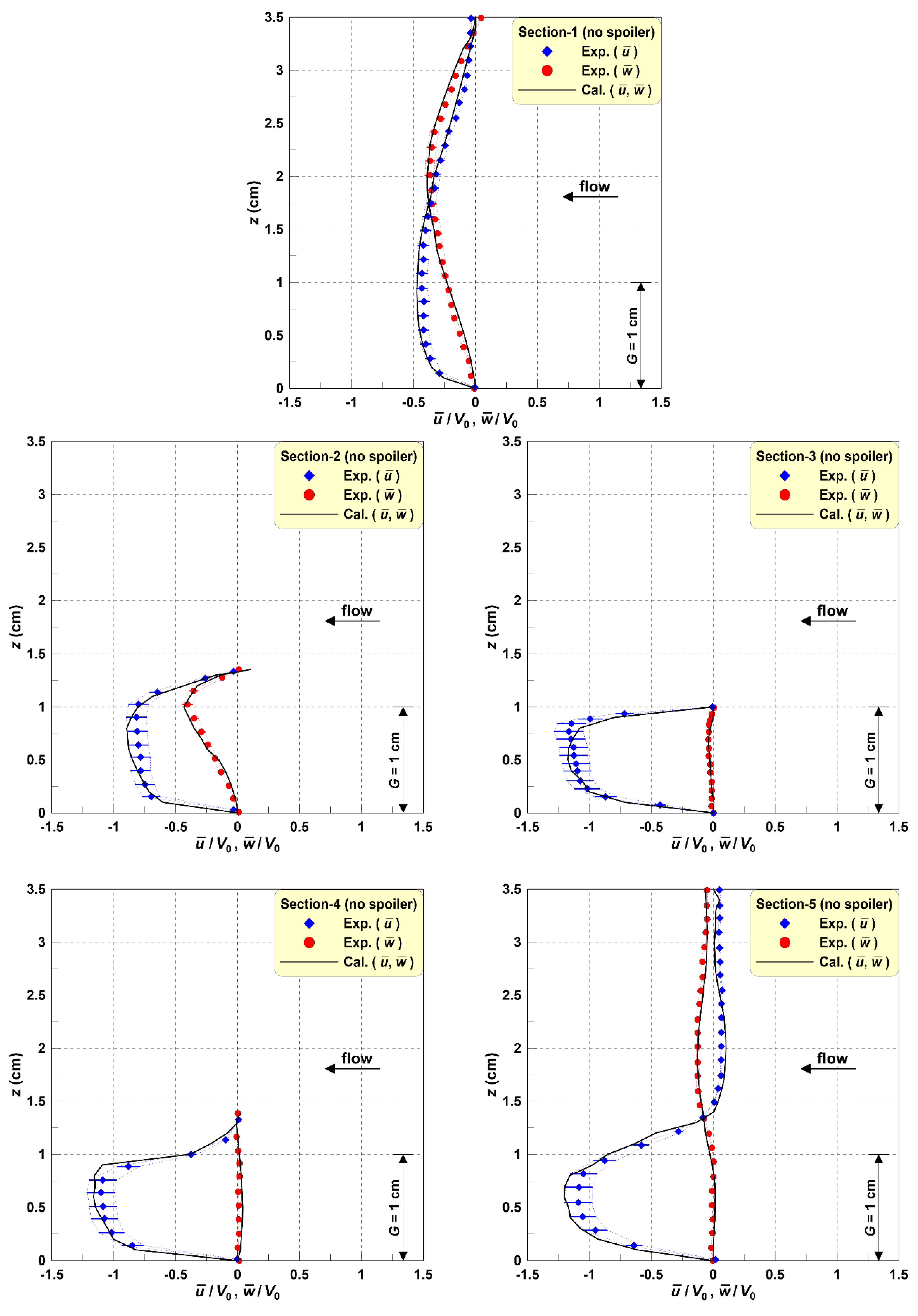
3.2.1. Velocity under Pipe with Spoiler

An NWT was developed based on the experiment tank of Oner [21] (Figure 10). A pipeline with a diameter of 5 cm was placed 1 cm from the bottom of the analysis zone with a depth of 32 cm, and a 1 cm long spoiler was attached to the top of the pipeline. In order to eliminate reflections created from the continuous flow at the boundaries on each side of the NWT, a source that created supplemental damper territory, radiation condition, and flow was placed suitably. The flow velocity was 19 cm/s and calculation grid sizes ( Δ x , Δ z ) in the horizontal and vertical directions were divided into 0.1 cm increments. Accordingly, the initial time interval Δ t was set to 1/2000 s, which was chosen to satisfy the Courant–Friedrichs–Lewy (CFL) and diffusive limit conditions.
Figure 11 shows the sections of velocity measurements below the pipeline. Numerical calculation values were determined to validate with the measured time-averaged velocities from the experiment by Oner [21]. Experimental and calculated results were compared (Figure 12 and Figure 13).
The average vertical velocity tended to increase when a spoiler was attached (Figure 13). The spoiler increased the projected area and, consequently, the horizontal velocity of the fluid leaving through the bottom of the pipeline and the vorticity at the front of the pipeline increased the average vertical velocity. Although the average horizontal and vertical velocities from numerical calculations tend to be slightly overestimated, the results reproduced the flow phenomenon described in the experiment [21]. Even though the comparisons were done under limited experimental conditions, they gave sufficient confirmation of the validity and effectiveness of LES-WASS-2D, which was used for numerical simulation in this study.

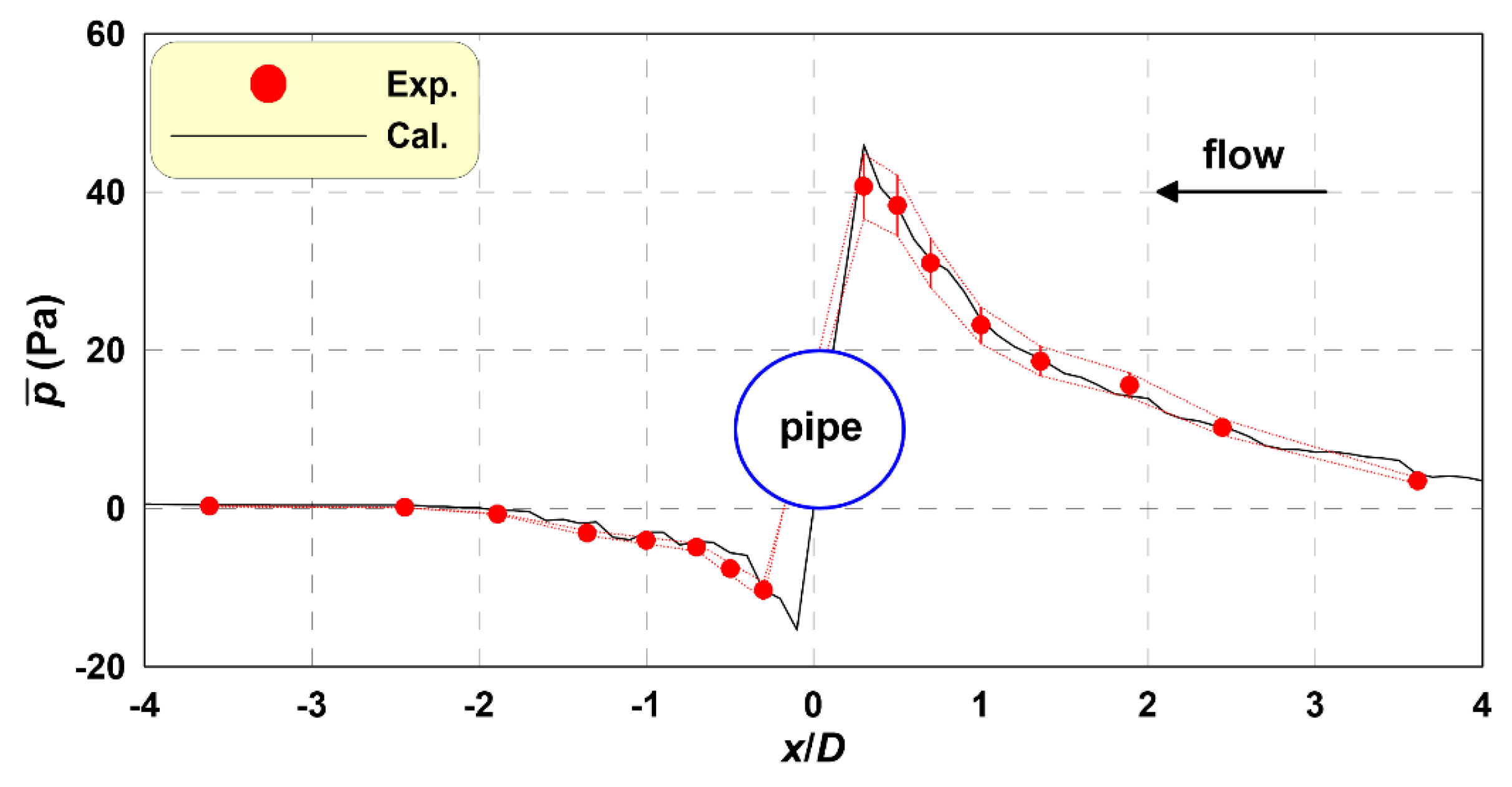
3.2.2. Bottom Pressure around Pipeline

The analysis zone in the NWT used was based on the experimental tank of Yang et al. [41] (Figure 14). In the analysis zone with a depth of 40 cm, a pipeline with a diameter of 9 cm was placed on a sand foundation with an average grain diameter ( d 50 ) of 0.56 mm and volume porosity ( γ v ) of 0.4. The remainder of the tank composition was the same as shown in Figure 10. The flow velocity ( V 0 ) was 24 cm/s and the horizontal and vertical calculation grid sizes ( Δ x , Δ z ) were set to 0.2 cm. Also, Δ t = 1 / 2000 s under laboratory conditions was used for the initial time intervals.
The results obtained showed positive pressure on the sand foundation surface near the front of the pipeline, but negative pressure at the rear end of the pipeline (Figure 15). This is owing to the flow creating pressure at the front of the pipeline, which increases the average pressure. At the rear end, a strong vortex caused a lower average pressure. In addition, based on test results, Yang et al. [41] proved that, as the pressure difference between the front and back of the pipe increased, local scouring also increased. It can be concluded that the numerical calculation results obtained in this study reproduced the experimental results well.
The numerical test results showed that the numerical model, LES-WASS-2D used in this study was appropriate for numerical simulation of the non-linear fluid–structure–seabed interaction.

3.2.3. Accuracy of Numerical Model

In addition to the qualitative reproducibility of the numerical models shown in Figure 12, Figure 13 and Figure 15, the statistical accuracies are indicated in Figure 16. To confirm the statistical accuracy of the numerical model, the normalized root mean square error (NRMSE) was calculated using Equation (7).
Under laboratory-scale conditions, the NRMSE of the time-averaged pressures on a sandy bed was 0.083, the NRMSE of the time-averaged horizontal velocity under the pipeline was 0.161, and the NRMSE of the time-averaged vertical velocity under the pipeline was 0.161, which verified the validity of the numerical analysis.
NRMSE = i = 1 N ( Ω i exp Ω i c a l ) 2 / i = 1 N ( Ω i exp ) 2
where N is the number of data, Ω i exp is the measured value, and Ω i cal is the calculated value.

3.3. Numerical Conditions

The validity and effectiveness of LES-WASS-2D were proven by comparing and verifying with hydraulic tests. Using LES-WASS-2D, an NWT was established (Figure 17), based on the previously performed hydraulic model test. The height of the sand foundation was chosen by considering the state of scouring in progress, obtained from hydraulic tests. The incident conditions and pipeline data were the same as with the hydraulic experiment. The vertical and horizontal computational grid sizes ( Δ x , Δ z ) were set to 0.2 cm each in the NWT. Also, Δ t = 1 / 2000 s was used for the initial time intervals, after which the Δ t was adjusted automatically each hour to satisfy CFL and the diffusive limit conditions.
The uncertainty of the numerical model (LES-WASS-2D) for steady flow conditions can be confirmed from the spatiotemporal distribution of flow velocity, turbulent kinetic energy, pressure, and vorticity in NWT. The spatial distribution of steady-state depth-averaged velocity, flow velocity, water surface elevation, and turbulent kinetic energy in NWT considering only a flat sandy bed without a pipeline is shown in Figure 18, and the spatial distributions of dynamic pressures and vorticity are shown in Figure 19, respectively. Here, the depth-averaged velocity in NWT is calculated using Equation (8), turbulent kinetic energy [42] using Equation (9), and the vorticity [43] on the xz plane using Equation (10).
V ¯ = h η v d z
K = 1 2 ( u 2 + w 2 ) + ( ν t C s Δ ) 2
ω x z = Γ A + Γ B + Γ C + Γ D 4 Δ x Δ z
{ Γ A = Δ x 2 ( u i 1 , k 1 + 2 u i , k 1 + u i + 1 , k 1 ) Γ B = Δ z 2 ( w i + 1 , k 1 + 2 w i + 1 , k + w i + 1 , k + 1 ) Γ C = Δ x 2 ( u i + 1 , k + 1 + 2 u i , k + 1 + u i 1 , k + 1 ) Γ D = Δ z 2 ( w i 1 , k + 1 + 2 w i 1 , k + w i 1 , k 1 )
where v is the flow velocity components; C s is the Smagorinsky’s constant; and Δ is the filter length scale taken as the square root of the computational grid area ( = Δ x Δ z ). In this study, the SGS simulation is performed with C s = 0.1 , which produces reasonable results for Smagorinsky’s model [29].
From Figure 18a, the depth-averaged velocity for the target flow velocity of 40 cm/s is approximately 38.5 cm/s, which is 96.25% and within ± 5% of the allowable error range. In Figure 18b, the flow velocity of the surface decreases, owing to the frictional resistance of the sandy bed and, after a certain depth, flow close to the target flow velocity. The turbulent kinetic energy increases near the surface owing to the interaction between the sandy bed and the flow, but is not large with the value 0.8 cm2/s2. There is some flow vibration near the point where the flow is generated (x = 800 cm), but the overall flow field remains steady. In particular, the flow at the point where the pipeline is placed (x = 400 cm) is very stable. In Figure 19a, the lower layer flow velocity is reduced owing to flow–sandy bed interaction, and the anti-clockwise vortex occurs because of the difference in flow velocity between the upper and lower layers. Vorticity on the surface of the sandy bed is a major factor causing scour, but its value is not greater than 6 1/s. The drop and rise of pressure in some parts near the flow generation point (x = 800 cm) are identified in Figure 19b. As the flow propagates in NWT, the pressure drop is caused by frictional resistance of the sandy bed. However, the dynamic pressure change of steady state NWT is very small at ±4 Pa.
On the basis of these quantitative figures, the observed hydraulic phenomena at steady flow conditions of NWT are generally reliable. Therefore, in this study, there would not be a significant problem in numerically analyzing the self-burial mechanism of the spoiler attached pipeline.

3.4. Numerical Results

3.4.1. Flow and Vortex Fields

The average flow and vortex field that occur periodically under steady flow conditions can be seen in Figure 20 (no spoiler) and Figure 21 (S/D = 0.3). Case (a) has early foundation conditions of equilibrium, while Cases (b), (c), and (d) applied the foundation conditions measured from previous hydraulic tests. Cases (b), (c), and (d) each show sand foundation cross-sections at 15 s, 120 s, and 2400 s at 40 cm/s, respectively, in steady flow conditions. Cases (b) and (c) show scouring in progress and (d) shows a state of equilibrium with almost no change in scour depth.
The pipeline projected area increased with spoilers and caused the flow velocity at the top and bottom of the pipe to increase and a strong vortex to form (Figure 20 and Figure 21). In particular, a strong vortex inside and outside of the sand foundation surface was created from strong flows leaving through the front of the pipeline (Figure 20a and Figure 21a). This occurrence lessened as the gap between the pipe and foundation surface increased as the scouring at the bottom of the pipeline progressed. The flow and vortex distributions formed around a pipeline had close relations with scouring near the pipeline, given steady flow conditions. Further, a strong vortex caused more scouring at the bottom of the pipeline.
The hydraulic experiment demonstrated that the early stages of scouring at the bottom of a pipeline were caused by flow and the vortex was large in fixed conditions where pipeline movement was prohibited. As scouring progressed, the vortex weakened at the sand foundation surface and the foundation cross-section displayed an equilibrium state. From these observations, the effect that a strong vortex at the bottom of a pipeline has on scouring can be understood. The vortex at the bottom of a pipeline according to S/D ratios (Figure 22) requires additional discussion.
The spatially-averaged values of time-averaged vortex values of a pipeline, determined using numerical simulations that considered initial foundation conditions, are portrayed (Figure 22). This analysis was completed using the domains in the front and back of the pipe (Figure 23). When a spoiler was attached, the vorticity at the front and rear end increased at the bottom of the pipeline. This was a similar result as demonstrated in Figure 20 and Figure 21. In addition, as the spoiler length increased, the projected area of the pipe increased and created a strong flow leaving at the bottom of the pipe. As the difference in flow and velocity increased within the sand foundation, it was assumed that a strong vorticity formed within and above the seabed as well. Therefore, when a spoiler is attached to a pipeline, strong vorticity at the front side of a pipe will occur, and consequently increase the scouring effects.
It was predicted that the analyzed scouring effects caused by vorticity would make the self-burial of pipelines with spoilers easier. This means that increased scouring at the bottom of a pipeline makes self-burial easier. Hence, the vorticity at the bottom of pipelines with spoilers can be considered as one of the main causes of self-burial.

3.4.2. Pressure Field and Force Acting on Pipe

The pattern-averaged dynamic pressures with a steady flow velocity of less than 40 cm/s were calculated (Figure 24 and Figure 25). These results also show numerical calculation results without a spoiler and with a spoiler with an S/D of 0.3. The ground conditions applied to numerical calculations were the same as the previously mentioned velocity and vortex fields. Case (a) shows the early stage ground condition; Cases (b) and (c) show scouring in progress with exposure to flow at 15 s and 120 s. Case (d) shows an equilibrium state with 2400 s of exposure to flow.
In order to understand the overall pressure distribution observed in Figure 24 and Figure 25, it should be analyzed in combination with pattern-averaged vorticity/velocity fields from Figure 20 and Figure 21. The pressure increased at the front side where flow resistance was high and pressure decreased at the rear side from strong vorticity owing to the slipstream (Figure 24, also refer to Figure 20). When a spoiler was attached (Figure 25), the projected area increased (Figure 21), which created a stronger flow leaving through the top and bottom of the pipe, and consequently caused stronger vorticity in the surroundings. This caused the pore water pressure within the seabed and the pressure behind the pipeline to decrease greatly. In addition, at the front side of the pipe, the spoiler junction created flow resistance, which increased the pressure near the pipe, creating positive (+) pressure throughout a large area. This phenomenon explained the increase in asymmetry of the pressure distribution near the pipeline when a spoiler was attached (Figure 25), compared with when a spoiler was absent (Figure 24). This asymmetric pressure distribution would cause the fluid force, which constantly acts on the pipeline, to be inclined to one specific direction. In order to discuss this matter in detail, the fluid force acting directly on the pipe owing to the pressure field around the pipe was calculated (Figure 25).
Yang et al. [41] demonstrated that scouring was greater with larger differences of pressure distribution at the front and rear end, near the seabed surface. Figure 24a and Figure 25a were used to compare pressures at the front and rear end of the pipeline near the seabed surface, while considering the presence of spoilers and the initial ground conditions, where scouring was the most vigorous. This comparison indicated that larger difference of pressures were present with a spoiler attached. Therefore, large local scouring would occur at the bottom of the pipeline with a spoiler attached and an equilibrium state with no more progression of scouring can result (Figure 24d and Figure 25d). In addition, as scouring progressed, pressure difference between the front and rear end of the pipeline, near the seabed surface, decreased and showed minimal pressure difference during an equilibrium state.
Figure 26 shows fluid force acting on the pipeline during a cycle of pressure pattern using numerical simulation with initial ground conditions, where (a) shows the horizontal force ( f x ) and (b) shows the vertical force ( f z ). When a spoiler was attached, the projected area and the fluid resistance increased (Figure 26a). This occurrence caused the front side pressure of the pipe to increase; the vorticity made the pressure drop at the rear end of the pipe, which increased f x significantly. When no spoiler was attached, the pressure structure had top and bottom symmetry, as seen from the pattern-averaged dynamic pressure field. This resulted in a small f z value (Figure 26b). Alternatively, f z was large for a pipeline with a spoiler, which had significant top and bottom asymmetry in the pressure structure. The pattern-averaged values are shown in Figure 27 for a quantitative analysis of fluid force acting on the pipeline.
A large increase in F x as the fluid resistance against the flow increased when a spoiler was attached (Figure 26 and Figure 27). When a spoiler was not attached, average F z was barely present; however, when a spoiler was attached, a large F z was present owing to the top and bottom of the pressure structure being asymmetrical. Therefore, when a pipeline with a spoiler was exposed to flow, it experienced a downward fluid force.
Numerical analysis on pressure distribution around the pipeline and fluid force acting on the pipe indicates that attaching a spoiler created a downward fluid force that acted directly on the pipeline, owing to the top and bottom asymmetry of the pressure distribution. This effect would be useful in the self-burial of subsea pipelines with spoiler attachments and was considered to be one of the major causes of self-burial of subsea pipelines.
The two major causes of self-burial of subsea pipelines derived from all the numerical analyses results are as follows. First, attaching a spoiler increased the projected area, which caused the flow velocity leaving the top and bottom of the pipe to increase. This created a strong vorticity within and above the seabed. Ultimately, large local scouring occurred at the bottom of the pipe. Second, attaching a spoiler increased the top and bottom asymmetry of the pressure structure near the pipeline and, as a consequence, a downward fluid force acted directly on the pipeline. These two major causes acted concurrently to drive the self-burial mechanism of pipelines with spoiler attachments.

4. Conclusions

In this study, laboratory experiments and numerical simulations were performed to clearly understand the self-burial mechanism of subsea pipelines under steady flow conditions. First, the scour characteristics at the bottom of the pipeline and the self-burial mechanism depending on spoiler attachments on pipelines were investigated through hydraulic model experiments. Next, the causes of self-burial of pipelines with spoilers were analyzed numerically from numerical model tests using the two-dimensional N–S solver. The major results found from these tests are listed below.
(1)
Hydraulic model tests with each side of a pipeline fixed showed that the equilibrium scour depth and scour range increased with the increase in the spoiler length to pipe diameter ratio (S/D).
(2)
Hydraulic model tests with non-fixed pipelines with spoilers, which could move freely, showed that the pipelines self-buried safely when exposed to steady flow. However, when the spoiler length was the longest (0.5D), unstable self-burial happened, where the pipeline was completely buried, but the spoiler was visible above the sand foundation.
(3)
In order to evaluate the suitability of the two-dimensional N–S solver, the numerical model, LES-WASS-2D used for numerical analyses; the velocity at the bottom of subsea pipelines with spoilers measured by Oner [21] and the pressure on the sand foundation surface right below the pipeline measured by Yang et al. [41] were compared and studied. The calculated results from the numerical model successfully reproduced the experimental results.
(4)
When a pipeline is built on a seabed, slipstream forms owing to the flow leaving from the top and bottom of the pipe. Further, a vortex forms near the pipe owing to flow resistance. Such a hydraulic phenomenon is exacerbated with a spoiler attachment.
(5)
Velocity and vorticity near the pipeline and the vorticity magnitude at the bottom of the pipe were numerically analyzed. Scouring due to the vorticity at the bottom of a pipeline accelerated even more with a spoiler, benefitting the self-burial process. Further, the pressure differences at the front and rear end of the pipeline near the seabed surface, which has a close relationship with scouring, increased greatly when a spoiler was attached.
(6)
Top and bottom asymmetry of the pressure structure that formed from spoiler attachments increased the downward fluid force acting on the pipe. This was also one of the major causes of self-burial of subsea pipelines.
(7)
The two major causes indicated in (5) and (6) above, working concurrently for the self-burial of pipelines with spoiler attachments, were numerically analyzed.
Through this study, it was possible to understand the self-burial mechanism of subsea pipeline with a spoiler, under the ideal condition of steady flow. However, to install the pipeline with a spoiler in the real ocean, where waves, tides, and ocean currents coexist, the self-burial performance must be reviewed by considering the nonlinear interactions among the factors of ocean physics. Also, in order to secure the safety of subsea pipelines through self-burial, the seabed of the corresponding ocean must be comprehensively surveyed beforehand. Using the field survey data, a hydraulic experiment or an accurate numerical analysis must be performed to review and select the appropriate spoiler specifications. This effort will maximize the self-burial effects of subsea pipelines with spoilers. Further, examination of spoiler material and structural integrity should not be overlooked. Lastly, after installation, the pipeline must be monitored meticulously to thoroughly study and analyze the self-burial process of a pipeline with a spoiler attachment.

Author Contributions

D.-S.H. and H.-J.J. designed the study concept; M.-J.K. and K.-H.J. performed the experiments; W.-D.L. and H.-S.K. performed the model simulations; All authors analyzed the results; W.-D.L. wrote the paper.

Funding

This research was part of a project entitled “Development of Coastal Erosion Control Technology” funded by the Ministry of Oceans and Fisheries, Korea. This work was supported by the National Research Foundation of Korea (NRF) grant funded by the Korea government (MSIT) (No. NRF-2018R1C1B6007461).

Conflicts of Interest

The authors declare no conflict of interest.

References

  1. Jensen, B.L.; Sumer, B.M.; Jensen, H.R.; Fredsøe, J. Flow around and forces on a pipeline near a scoured bed in steady stream. J. Offshore Mech. Arct. Eng. 1990, 112, 206–312. [Google Scholar] [CrossRef]
  2. Sumer, B.M.; Mao, Y.; Fredsøe, J. Interaction between vibrating pipe and erodible bed. J. Waterw. Port Coast. Ocean Eng. 1988, 114, 81–92. [Google Scholar] [CrossRef]
  3. Sumer, B.M.; Fredsøe, J. Scour below pipelines in waves. J. Waterw. Port Coast. Ocean Eng. 1990, 116, 307–323. [Google Scholar] [CrossRef]
  4. Sumer, B.M.; Fredsøe, J. Onset of scour below a pipeline exposed to waves. Int. J. Offshore Polar Eng. 1991, 1, 189–194. [Google Scholar]
  5. Sumer, B.M.; Fredsøe, J. Scour around pile in combined waves and currents. J. Hydraul. Eng. 2001, 127, 403–411. [Google Scholar] [CrossRef]
  6. Yang, G.; Ye, J. Wave & current-induced progressive liquefaction in loosely deposited seabed. Ocean Eng. 2017, 142, 303–314. [Google Scholar]
  7. Tong, D.; Liao, C.; Chen, J.; Zhang, Q. Numerical simulation of a sandy seabed response to water surface waves propagating on current. J. Mar. Sci. Eng. 2018, 6, 88. [Google Scholar] [CrossRef] [Green Version]
  8. Sumer, B.M.; Fredsøe, J. Advanced Series on Ocean Engineering 17. In The Mechanics of Scour in the Marine Environment; World Scientific: Singapore, 2002; p. 536. [Google Scholar]
  9. Sumer, B.M. Advanced Series on Ocean Engineering 39. In Liquefaction around Marine Structures; World Scientific: Singapore, 2014; p. 472. [Google Scholar]
  10. Hulsbergen, C.H. Stimulated self-burial of submarine pipelines. In Proceedings of the 16th Offshore Technology Conference, Houston, TX, USA, 7–9 May 1984; OTC 4667. pp. 171–177. [Google Scholar]
  11. Hulsbergen, C.H.; Bijker, H. Effect of spoilers submarine pipeline stability. In Proceedings of the 21st Offshore Technology Conference, Houston, TX, USA, 1–4 May 1989; OTC 6154. pp. 337–350. [Google Scholar]
  12. Chiew, Y. Effect of spoilers on scour at submarine pipelines. J. Hydraul. Eng. 1990, 118, 1311–1317. [Google Scholar] [CrossRef]
  13. Chiew, Y. Effect of spoilers on wave-induced scour at submarine pipelines. J. Waterw. Port Coast. Ocean Eng. 1993, 417, 417–428. [Google Scholar] [CrossRef]
  14. Zhao, J.; Wang, X. CFD numerical simulation of the submarine pipeline with a spoiler. J. Offshore Mech. Arct. Eng. 2009, 131, 031601. [Google Scholar] [CrossRef]
  15. Sumer, B.M.; Truelsen, C.; Shchmann, T.; Fredsøe, J. Onset of scour below pipelines and self-burial. Coast. Eng. 2001, 42, 313–335. [Google Scholar] [CrossRef]
  16. Alam, M.S.; Cheng, L. A 2-D model to predict time development of scour below pipelines with spoiler. In 2nd International Symposium on Computational Mechanics and 12th International Conference on the Enhancement and Promotion of Computational Methods in Engineering and Science; American Institution of Physics: New York, NY, USA, 2010; pp. 993–998. [Google Scholar]
  17. Yang, L.; Shi, B.; Guo, Y.; Wen, X. Calculation and experiment on scour depth for submarine pipeline with a spoiler. Ocean Eng. 2012, 55, 191–198. [Google Scholar] [CrossRef]
  18. Yang, L.; Guo, Y.; Shi, B.; Kuang, C.; Xu, W.; Cao, S. Study of scour around submarine pipeline with a rubber plate or rigid spoiler in wave conditions. J. Waterw. Port Coast. Ocean Eng. 2012, 138, 484–490. [Google Scholar] [CrossRef]
  19. Abbasi, S.; Masoomi, M.; Arjmandi, S.A. Impact of a Single Spoiler on Scouring Depth Status Beneath a River Crossing Inclined Pipeline. Eng. Technol. Appl. Sci. Res. 2018, 8, 3316–3320. [Google Scholar]
  20. Cheng, L.; Chew, L. Modelling of flow around a near-bed pipeline with a spoiler. Ocean Eng. 2003, 30, 1595–1611. [Google Scholar] [CrossRef]
  21. Oner, A.A. The flow around a pipeline with a spoiler. Proc. Inst. Mech. Eng. Part C J. Mech. Eng. 2010, 224, 109–121. [Google Scholar] [CrossRef]
  22. Han, Y. Study on the submarine pipeline with flexible spoilers. Key Eng. Mater. 2012, 501, 431–435. [Google Scholar] [CrossRef]
  23. Zhu, H.; Qi, X.; Lin, P.; Yang, Y. Numerical simulation of flow around a submarine pipe with a spoiler and current-induced scour beneath the pipe. Appl. Ocean Res. 2013, 41, 87–100. [Google Scholar] [CrossRef]
  24. Oner, A.A. Numerical investigation of flow around a pipeline with a spoiler near a rigid bed. Adv. Mech. Eng. 2016, 8, 1–13. [Google Scholar] [CrossRef] [Green Version]
  25. Barendse, C.A.M. Hydrodynamic Forces on a Near-Bed Offshore Pipeline with Spoiler, during the Selfburying Process. Master’s Thesis, TU Delft, Delft, The Netherlands, 1988; p. 193. [Google Scholar]
  26. Bakhtiary, A.D.; Zeinali, M. Numerical simulation of hydrodynamic forces on submarine pipeline with a spoiler. In Proceedings of the 8th International Conference on Coasts, Ports and Marine Structures (ICOPMAS), Ports and Marine Organization, Tehran, Iran, 24–26 November 2008; Volume 8, pp. 1–12. [Google Scholar]
  27. Nortek, The Comprehensive Manual—Velocimeters. Nortek Underwater Instruments, 2018. Available online: http://nortekgroup.com (accessed on 25 November 2019).
  28. Hur, D.S.; Lee, K.H.; Choi, D.S. Effect of the slope gradient of submerged breakwaters on wave energy dissipation. Eng. Appl. Comput. Fluid Mech. 2011, 5, 83–98. [Google Scholar] [CrossRef] [Green Version]
  29. Smagorinsky, J. General circulation experiments with the primitive equation. Mon. Weather Rev. 1963, 91, 99–164. [Google Scholar] [CrossRef]
  30. Sakakiyama, T.; Kajima, R. Numerical simulation of nonlinear wave interacting with permeable breakwater. In Proceedings of the 23rd International Conference on Coastal Engineering, Venice, Italy, 4–9 October 1992; pp. 1517–1530. [Google Scholar]
  31. Ergun, S. Fluid flow through packed columns. Chem. Eng. Prog. 1952, 48, 89–94. [Google Scholar]
  32. Liu, S.; Masliyah, J.H. Non-linear flows in porous media. J. Non-Newton. Fluid Mech. 1999, 86, 229–252. [Google Scholar] [CrossRef]
  33. Hinatsu, M. Numerical simulation of unsteady viscous nonlinear waves using moving grid system fitted on a free surface. J. Kansai Soc. Nav. Archit. 1992, 217, 1–11. [Google Scholar]
  34. Brorsen, M.; Larsen, J. Source generation of nonlinear gravity wave with boundary integral equation method. Coast. Eng. 1987, 11, 93–113. [Google Scholar] [CrossRef]
  35. Lee, W.D.; Yoo, Y.J.; Jeong, Y.M.; Hur, D.S. Experimental and numerical analysis on hydraulic characteristics of coastal aquifers with seawall. Water 2019, 11, 2343. [Google Scholar] [CrossRef] [Green Version]
  36. Ohyama, T.; Nadaoka, K. Modeling the transformation of nonlinear waves passing over a submerged dike. In Proceedings of the 23rd International Conference on Coastal Engineering, Venice, Italy, 4–9 October 1992; pp. 526–539. [Google Scholar]
  37. Hirt, C.W.; Nichols, B.D. Volume of fluid (VOF) method for the dynamics of free boundaries. J. Comput. Phys. 1981, 39, 201–225. [Google Scholar] [CrossRef]
  38. Hur, D.S.; Lee, W.D.; Cho, W.C.; Jeong, Y.H.; Jeong, Y.M. Rip current reduction at the open inlet between double submerged breakwaters by installing a drainage channel. Ocean Eng. 2019, 193, 106580. [Google Scholar] [CrossRef]
  39. Lee, W.D.; Jeong, Y.H.; Jeon, H.S. Groundwater flow analysis in a coastal aquifer with the coexistence of seawater and freshwater by using a non-hydrostatic pressure model. J. Coast. Res. 2019, 91, 121–125. [Google Scholar] [CrossRef]
  40. Petit, H.A.H.; Tonjes, P.; ven Gent, M.R.A.; van den Bosch, P. Numerical simulation and validation of plunging breakers using a 2D Navier–Stokes model. In Proceedings of the 24th International Conference on Coastal Engineering, Kobe, Japan, 23–28 October 1994; pp. 511–524. [Google Scholar]
  41. Yang, L.; Shi, B.; Guo, Y.; Zhang, L.; Zhang, J.; Han, Y. Scour protection of submarine pipelines using rubber plates underneath the pipes. Ocean Eng. 2014, 84, 176–182. [Google Scholar] [CrossRef] [Green Version]
  42. Christensen, E.D. Large eddy simulation of spilling and plunging breakers. Coast. Eng. 2006, 53, 463–485. [Google Scholar] [CrossRef]
  43. Raffel, M.; Willert, C.E.; Wereley, S.T.; Kompenhans, J. Particle Image Velocimetry; Springer Verlag: Berlin, Germany, 2007; p. 448. [Google Scholar]
Figure 1. Concept sketch of structural risks of the subsea pipeline by local scour.
Jmse 07 00456 g001
Figure 2. Schematic of water tank including pipeline with spoiler, set up for laboratory experiments.
Jmse 07 00456 g002
Figure 3. Arrangement of spoiler on pipeline: (a) No spoiler, (b) S/D = 0.3, (c) S/D = 0.5.
Jmse 07 00456 g003
Figure 4. Measured points of acoustic Doppler velocimeter (ADV) for determining incident flow velocity: (a) side view, (b) plan view.
Jmse 07 00456 g004
Figure 5. Comparison of scour depths under fixed-pipeline in time domain. The black circle is Run-1 with no spoiler; the blue square is Run-2 with a spoiler length to pipe diameter ratio (S/D) of 0.3; and the red triangle is Run-3 with an S/D of 0.5.
Jmse 07 00456 g005
Figure 6. Equilibrium profiles of sandy bed under steady flow in case of fixed-pipeline: (a) Run-1 (no spoiler), (b) Run-2 (S/D = 0.3), (c) Run-3 (S/D = 0.5). The yellow circle represents the cross section of the subsea pipeline, the black grid sizes are 1 cm (L) × 1 cm (H), and the mint-colored grid sizes are 10 cm (L) × 10 cm (H).
Jmse 07 00456 g006
Figure 7. Comparison of burial depth of free-pipeline in time domain. The black dot represents Run-1 with no spoiler, the blue square represents Run-2 with a spoiler length to pipe diameter ratio of 0.3, and the red triangle represents Run-3 with an S/D of 0.5.
Jmse 07 00456 g007
Figure 8. Equilibrium profiles of seabed under steady flow in case of free-pipeline: (a) Run-1 (no spoiler), (b) Run-2 (S/D = 0.3), (c) Run-3 (S/D = 0.5). The yellow circle is the subsea pipeline cross-section, the black grid sizes are 1 cm × 1 cm, and the mint-colored grid sizes are 10 cm × 10 cm.
Jmse 07 00456 g008
Figure 9. Spatial distribution of bed elevations and location of pipeline in equilibrium state: (a) Run-1 (no spoiler), (b) Run-2 (S/D = 0.3), (c) Run-3 (S/D = 0.5).
Jmse 07 00456 g009
Figure 10. Definition sketch of the numerical water tank (NWT) based on the experiment water tank [21].
Jmse 07 00456 g010
Figure 11. Measured sections of velocities under pipeline.
Jmse 07 00456 g011
Figure 12. Comparison between measured [21] and calculated time-averaged velocities under the pipeline without a spoiler. The markers represent the experimental results and the solid line represents the calculated results. The circles are the horizontal velocities; the diamonds are the vertical velocities. The error bars have an error range of ± 10%.
Jmse 07 00456 g012
Figure 13. Comparison between measured [21] and calculated time-averaged velocities under the pipeline with a spoiler.
Jmse 07 00456 g013
Figure 14. Definition sketch of analysis zone in NWT based on the experimental water tank [41].
Jmse 07 00456 g014
Figure 15. Comparison between measured and calculated time-averaged pressures on a sandy bed. The red circle represents values measured by Yang et al. [41] and the black solid line represents the numerically calculated values. The error bars have an error range of ± 10%.
Jmse 07 00456 g015
Figure 16. Statistical comparisons between measured and calculated values: (a) pressures on sandy bed, (b) horizontal velocity under pipeline, (c) vertical velocity under pipeline. The solid line shows the trend line, and the dotted line area indicates within error range of ± 10%. The blue circle shows the case with no spoiler, the red triangle shows the case with S/D = 0.2. RMSE, root mean square error; NRMSE, normalized RMSE.
Jmse 07 00456 g016
Figure 17. Definition sketch of NWT based on laboratory experiments.
Jmse 07 00456 g017
Figure 18. Spatial distributions of (a) depth-averaged velocities and (b) velocities, water surface elevations, and turbulent kinetic energy at steady state in NWT without a pipeline. The colors grow redder when K increase.
Jmse 07 00456 g018
Figure 19. Spatial distributions of (a) vorticities and (b) dynamic pressures at steady state in NWT without a pipeline. Blue tones represent clockwise vortex and negative pressure distribution; red tones represent anti-clockwise vortex and positive pressure distribution.
Jmse 07 00456 g019
Figure 20. Spatial distributions of pattern-averaged velocities and vorticities around pipeline without a spoiler: (a) t = 0 s (initial condition), (b) t = 15 s (in the process of scouring), (c) t = 120 s (in the process of scouring), (d) t = 2400 s (equilibrium state). Blue tones represent clockwise vortex; red tones represent anti-clockwise vortex.
Jmse 07 00456 g020
Figure 21. Spatial distributions of pattern-averaged velocities and vorticities around pipeline with a spoiler in the case of S/D = 0.3: (a) t = 0 s (initial condition), (b) t = 15 s (in the process of scouring), (c) t = 120 s (in the process of scouring), (d) t = 2400 s (equilibrium state).
Jmse 07 00456 g021
Figure 22. Comparison of spatial averaged vorticities owing to S/D in front and rear side under pipeline. The lateral axis is the ratio of spoiler length to pipe diameter (S/D) and the longitudinal axis is the spatial-average vortex ( ω ¯ x z ). The circle is the front, and the triangle is the rear end average vorticity.
Jmse 07 00456 g022
Figure 23. Estimated domains under pipeline for spatial averaged vorticity: (a) Rear side, (b) Front side.
Jmse 07 00456 g023
Figure 24. Spatial distributions of pattern-averaged dynamic pressures around the pipeline without a spoiler: (a) t = 0 s (initial condition), (b) t = 15 s (in the process of scouring), (c) t = 120 s (in the process of scouring), (d) t = 2400 s (equilibrium state). Blue tones represent negative pressure distribution and red tones represent positive pressure distribution.
Jmse 07 00456 g024aJmse 07 00456 g024b
Figure 25. Spatial distributions of pattern-averaged dynamic pressures around the pipeline with a spoiler where S/D = 0.3: (a) t = 0 s (initial condition), (b) t = 15 s (in the process of scouring), (c) t = 120 s (in the process of scouring), (d) t = 2400 s (equilibrium state).
Jmse 07 00456 g025aJmse 07 00456 g025b
Figure 26. Comparison of fluid force due to S/D at the pipeline: (a) horizontal force ( f x ), (b) vertical force ( f z ). The black solid line shows the case with no spoiler, the blue circle shows the case with S/D = 0.3, and the red triangle shows the case with S/D = 0.5.
Jmse 07 00456 g026
Figure 27. Comparison of mean force due to S/D at the pipeline. The black circle represents the mean horizontal force ( F x ) and the red inverted triangle represents the vertical force ( F z ).
Jmse 07 00456 g027
Table 1. Experimental conditions.
RunVelocityPipeSpoiler
DiameterLengthRatio
V0 (cm/s)D (cm)S (cm)S/D
1405-
21.50.3
32.50.5
Table 2. Material conditions of pipe model.
SortPipe Model
Density (g/cm3)1.45
Mass per length (g/cm)8

