Article

Design of an Adaptive Sliding Mode Control for a Micro-AUV Subject to Water Currents and Parametric Uncertainties

Tecnologico de Monterrey, School of Science and Engineering, Av. Eugenio Garza Sada 2501 Sur Monterrey, Nuevo Leon 64849, Mexico
*
Author to whom correspondence should be addressed.
J. Mar. Sci. Eng. 2019, 7(12), 445; https://doi.org/10.3390/jmse7120445
Submission received: 24 October 2019 / Revised: 30 November 2019 / Accepted: 30 November 2019 / Published: 4 December 2019
(This article belongs to the Special Issue Advances in Oceanic and Mechatronic Systems Engineering)

Abstract

:
This paper addresses the design of an adaptive sliding mode control for an autonomous underwater vehicle with the objective to reject bounded internal and external perturbations. The proposed control is used to achieve velocity regulation and autonomous path-following using waypoints. Each task is successfully performed in the presence of parametric uncertainties and irrotational water currents. Due to complex dynamics and random external perturbations, underwater vehicles need robust control. The closed-loop stability and finite-time convergence of the system are demonstrated using the Lyapunov direct method. To provide a detailed and realistic testing environment for the proposed adaptive controller, a dynamic model of the vehicle using the Lagrange method is derived where all underwater effects are included. On that basis, the proposed adaptive sliding mode controller is compared to its non-adaptive equivalent and PD (Proportional Derivative) computed torque control. The simulation results demonstrate that the proposed adaptive control has better robustness and precision for this particular type of vehicle.

1. Introduction

Autonomous Underwater Vehicles (AUVs) play an important role today in the offshore industry or ocean exploration as they can reach places where human intervention is dangerous or even impossible. Their tasks can go from simple visual inspection to more complex interactions [1]. These vehicles are subject to uncertainties and unexpected dynamics due to their environment such as water currents [2,3], turbulence, tether cable forces [4] or obstacles. Furthermore, the control must deal with model uncertainties in geometry, mass, damping, actuation forces and noisy measurements. In real operating conditions, the control must remain robust again all these perturbations sources to ensure precise navigation. For the specific case of micro AUVs, as their mass is inferior to 4.5 kg [5], the effect of any external disturbance is much greater than for classical heavy underwater vehicles. This constraint requires control for this category of vehicles to have good performance in terms of disturbance rejection and tracking error. Underwater vehicles are generally modeled as 6 degrees of freedom (DOF) systems. The classical denomination for each DOF is: surge, sway, heave, roll, pitch and yaw [6]. In literature, majority of the models are derived from Newton/Euler approach [7,8,9].
Over the past 20 years, many linear methods have been tested on AUVs such as PID (Proportional Integral Derivative) [10,11], PD [12] or optimal quadratic control [13]. In [14], the closed-loop behavior of an AUV model is first linearized by computed torque control-like method to apply then a PID controller. Even if this reference shows the feasibility of attitude feedback based on Euler parameters (Quaternions), no disturbance is applied to investigate robustness. However, the main drawback of all linear control methods is still the requirement of precise knowledge of the system and limited control gains to maintain robustness. Sliding mode control (SMC) is a widely used control method [15,16,17]. This type of control leads the states of the system to a sliding surface resulting in the global asymptotic convergence of the tracking error. Finite-time convergence can be ensured if the boundaries of the perturbations are known. However, these boundaries are often overestimated which can lead to control energy waste. The main issue for SMC is that robustness is only guaranteed using high switching gains. Hence, when the system states reach the defined sliding surface, chattering appears on the command signal and can quickly damage the propulsion system.
In [8,18,19,20], adaptive control is implemented using linearization methods with PD control and the system regressor function to compensate model uncertainties. Results highlight the fact that poor estimation of the model parameters can degrade rapidly the robustness of adaptive control. Another adaptive PID control is presented in [21] where the uncertainties upper bounds are estimated online. The method succeeds but suffers a significant loss of robustness when facing noisy measurements. Robust adaptive control is used in [22] to drive in the ( x y ) plane an AUV model trying to avoid especially side slip during a path-following task. Nevertheless, no external perturbation problem is addressed.
A class of adaptive sliding mode control (ASMC) has been also applied for AUV motion control [23] to avoid high switching gains and add robustness compared to conventional SMC. Chattering when the sliding variable is close to the sliding surface can be reduced by introducing a boundary layer. In the aforementioned reference, the dead zone of the thruster is also considered and ASMC successfully deals with this non-linearity. Nonetheless, only constant perturbations are addressed in this reference.
In [24], adaptive non-singular integral terminal sliding mode control is implemented for trajectory tracking of a 6 DOF AUV model. Time-varying external disturbances are added to apprehend robustness but they remain deterministic; no transient or random components are added to simulate the underwater environment.
Another recent approach investigated is the adaptive high order sliding mode control in [25]. This method derived from adaptive sliding mode control maintains both the efficiency and robustness of the ASMC approach. Good results are obtained especially when simulating the failure of one of the thrusters. Though, the main drawback of these ASMC approaches remains as higher command forces to keep robustness and chattering.
The problem addressed in this work is that micro AUVs suffer much more from external perturbations than conventional heavier vehicles. The proposed controller provides robustness and fast adaptive control dynamics to ensure the precise navigation of the micro-AUV.
The main contribution of this work is the design of a robust controller based on a class of adaptive sliding mode control to ensure the rejection of bounded internal and external perturbations, demonstrated by the Lyapunov direct method. The proposed control performs velocity regulation and a waypoint following task on a detailed micro underwater vehicle model based on the Lagrange method. Finally, the feasibility and efficiency of the proposed controller are tested and compared to other conventional control methods under three scenarios via simulations where realistic disturbances are applied to the vehicle.
The paper outline is the following: Section 2 presents a modeling method for an underwater vehicle. The next Section 3 develops the ASM controller on the dynamic model and addresses its stability using a Lyapunov approach. Then, Section 4 presents the theoretical basis for autonomous path-following task. Finally, Section 5 exposes the simulations results and the associated analysis.

2. Underwater Vehicle Model
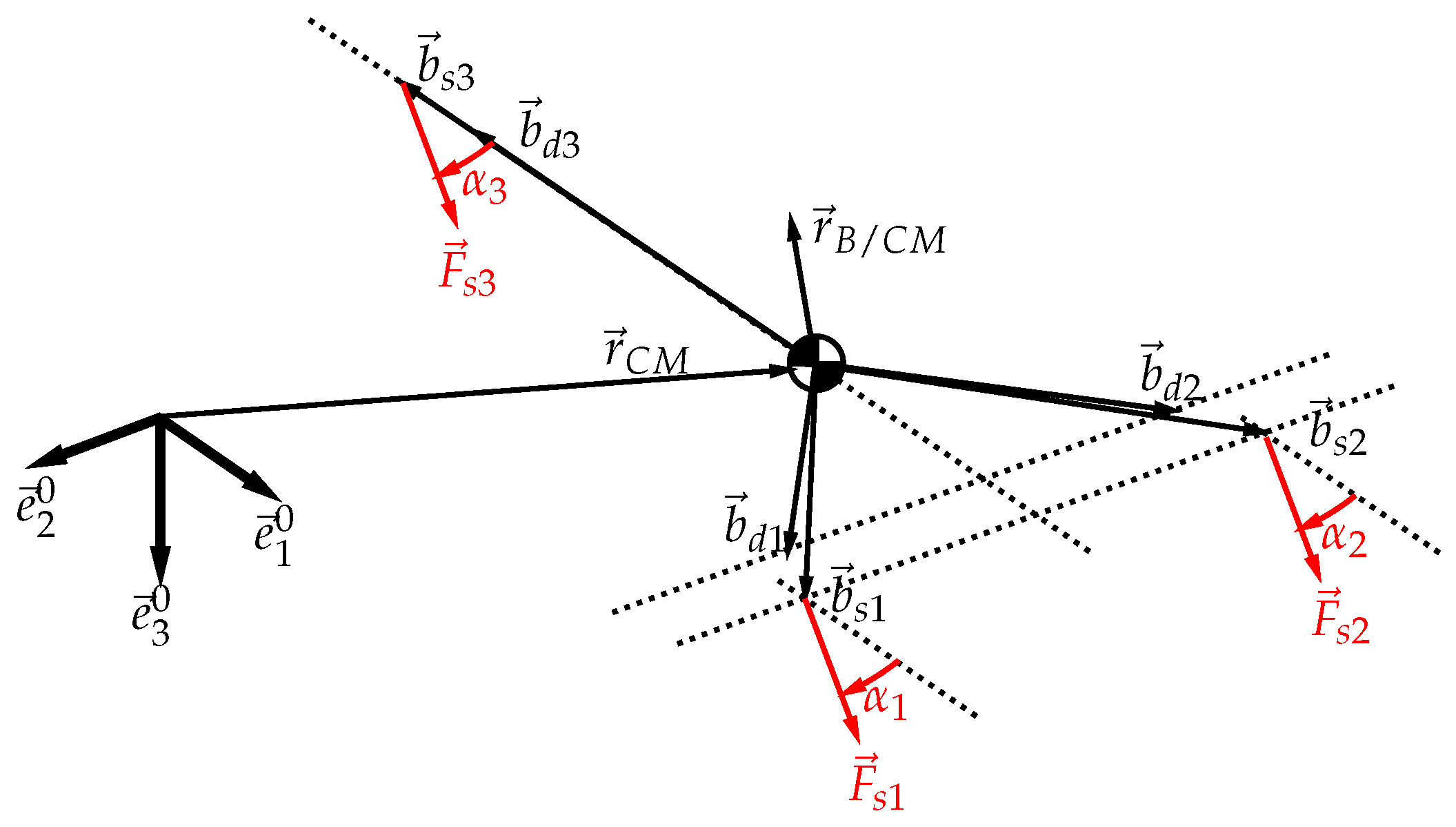
2.1. Model Design

In this section, a dynamical model of an underwater vehicle-type micro-AUV using the Lagrange method for the computation of the equations of motion is derived. The physical prototype is a 2.5 kg AUV of 0.4 m length and 0.28 m width. A schematic representation of the model is presented in Figure 1 defining the world frame, the body-fixed frame, and the rotation parameters.
Kinematics: First, two frames are needed to describe the motion of the system:
  • e ̲ 0 : world frame attached to earth surface
  • e ̲ 1 : body-fixed frame attached to the AUV
The axis [ e ̲ 1 0 , e ̲ 2 0 , e ̲ 3 0 ] of the world frame are oriented using the classical NED configuration (North, East, Deep). The same axis attached to the body of the vehicle are oriented in the following configuration: forward, right, dive (see Figure 1).
The chosen parametric representation of the cosine matrix defining the rotation sequence from the world frame to the body-fixed frame is the Tait-Bryant sequence ( 1 , 2 , 3 ) corresponding to Roll-Pitch-Yaw angles. The corresponding rotations parameters are:
θ ̲ = [ ϕ ( t ) , θ ( t ) , ψ ( t ) ] T
The final cosine matrix is defined as A ̲ 10 :
A ̲ 10 = C θ C ψ C ψ S θ S ϕ + C ϕ S ψ C ϕ C ψ S θ + S ϕ S ψ C θ S ψ C ϕ C ψ S θ S ϕ S ψ C ψ S ϕ + C ϕ S θ S ψ S θ C θ S ϕ C θ C ϕ
Assumption is made here that π 2 < θ ( t ) < π 2 to avoid any singularity in A ̲ 10 .
The coordinates transformation between the frames 0 and 1 is expressed by:
e ̲ 1 = A ̲ 10 e ̲ 0
The rotation vector 10 ω of the body-fixed frame with respect to the world frame is expressed in the body-fixed frame e ̲ 1 as:
10 ω 1 = sin ( ψ ) θ ˙ + cos ( θ ) cos ( ψ ) ϕ ˙ cos ( ψ ) θ ˙ cos ( θ ) sin ( ψ ) ϕ ˙ sin ( θ ) ϕ ˙ + ψ ˙ T
One can now define the position vector of the AUV center of mass:
r C M = r ̲ C M 0 T e ̲ 0
where
r ̲ C M 0 T = [ x ( t ) , y ( t ) , z ( t ) ]
The vector of generalized coordinates q ̲ is defined by [ x y z ϕ θ ψ ] T . Finally, the velocity vector of the vehicle in its body-fixed frame containing the linear and angular terms is V ̲ = [ u , v , w , p , q , r ] T where:
u v w = r ̲ ˙ C M 0 . A ̲ 10 T
p q r = 10 ω 1
Masses and inertia: The behavior of an underwater vehicle is deeply influenced by the hydrodynamic effects. The main components of these forces are hydrodynamic damping and added mass due to fluid displacement around the moving vehicle [6].
Based on this assumption, m 1 is defined as the AUV mass. m a u , m a v and m a w are the added mass parameters in the different body-fixed axis e 1 1 , e 2 1 and e 3 1 . Thus, the total time invariant inertia matrix C M 1 J ̲ (defined at the CM of the body-fixed frame) is defined by:
C M 1 J ̲ = J x x 1 + J x x a 0 0 0 J y y 1 + J y y a 0 0 0 J z z 1 + J z z a
The angular momentum is now defined in the body-fixed frame using the rotation parameters and inertia:
H C M 1 = ( C M 1 J ̲ + C M a J ̲ ) . 10 ω 1

2.2. Lagrange Method

In this section, the kinetic and potential energies of the system as well as the external forces are derived to use the Lagrange equation and compute the equations of motion.
Kinetic energy: First, one can define the kinetic energy T as:
T = 1 2 m r ˙ C M 2 + m a u u 2 + m a v v 2 + m a w w 2 + 1 2 10 ω 1 . H C M 1
Potential energy: As the underwater vehicle model does not include any stiffness due to joints, the only two sources of potential energy are gravity and buoyancy applied respectively to the center of mass and center of buoyancy.
The gravity vector in the world frame is g = [ 0 , 0 , g ] e ̲ 0 (positive z axis points toward sea floor). Then, potential due to gravity is:
V g = m 1 ( g . r C M )
One can now define the point B belonging to the body-fixed frame as the point of application of the Buoyancy force, its coordinates are relative and defined in function of the center of mass position:
r B / C M 1 = [ x B / C M , y B / C M , z B / C M ] e ̲ 1
as in (14), the Buoyancy potential is expressed by:
V b = ρ V g . ( r C M + r B / C M 1 . A ̲ 10 )
with ρ the fluid density [ k g / m 3 ] and V the underwater vehicle submerged volume [ m 3 ] . The total potential energy is then V = V g + V b .
Non-conservative forces: Non-conservative forces applying on the vehicle are propellers thrust and hydrodynamic damping. The AUV has m propellers acting in the ( x y ) plane for surge, sway and yaw control and n propellers acting in the z direction for roll, pitch, and dive control.
First, let us define the link vectors b s i and b d j with i [ 1 : m ] and j [ 1 : n ] defining the relative positions of the different propellers (see Figure 2) with respect to the center of mass in the body-fixed frame:
b s i = [ b s i x , b s i y , b s i z ] e ̲ 1
b d j = [ b d j x , b d j y , b d j z ] e ̲ 1
The corresponding propellers force vectors F s i and F d j acting on the underwater vehicle are written in this form:
F s i = [ F s i cos ( α i ) , F s i sin ( α i ) , 0 ] e ̲ 1
F d j = [ 0 , 0 , F d j ] e ̲ 1
where α i is the angle between the propulsion direction of the i t h propeller and the x-axis of the body-fixed frame in its ( x y ) plane.
Now let us define the damping forces and moments acting on the center of mass of the underwater vehicle. These forces depend on the linear and rotational speed of the AUV in its body-fixed frame. Moreover, a quadratic model [6] is used to compute the hydrodynamic damping:
D u = X u | u | . | u | . u X u . u D v = Y v | v | . | v | . v Y v . v D w = Z w | w | . | w | . w Z w . w D p = K p | p | . | p | . p K p . p D q = M q | q | . | q | . q M q . q D r = N r | r | . | r | . r N r . r
where X u | u | , Y v | v | , Z w | w | , K p | p | , M q | q | and N r | r | are the quadratic coefficients and X u , Y v , Z w , K p , M q and N r the linear coefficients. Then the damping forces and moments acting on the center of mass are written as:
F D = [ D u , D v , D w ] e ̲ 1
M D = [ D p , D q , D r ] e ̲ 1
Thus, the generalized non-conservative external and internal forces Q e x and Q i n are synthesized in these expressions:
Q e x = i = 1 m q ̲ r C M + b s i . A ̲ 10 e ̲ 0 T . ( F s i . A ̲ 10 ) + j = 1 n q ̲ r C M + b d j . A ̲ 10 e ̲ 0 T . ( F d j . A ̲ 10 )
and
Q i n = r C M q ̲ T . ( F D . A ̲ 10 ) + θ ̲ q ̲ T . ( M D . A ̲ 10 )
Finally, the generalized non-conservative forces vector is defined as Q n c = Q i n + Q e x .
Equations of motion: Since the system is unconstrained and so described using 6 generalized independent coordinates (vector q ̲ ), it is proper to use the so-called Lagrangian equations of motion to describe the dynamics of the system:
d d t T , q ˙ ̲ T , q ̲ + V , q ̲ = Q ̲ n c T
where T , q ̲ and T , q ˙ ̲ 6 × 1 are respectively the derivatives of the system kinetic energy with respect to each generalized coordinate or its time derivative. V , q ̲ 6 × 1 is the vector derivative of the potential energy with respect to each general coordinate.
The Equation (24) can be rewritten in the following form:
M ̲ ( q ̲ ) q ¨ ̲ + H ̲ ( q ̲ , q ˙ ̲ ) = S ̲ ( q ̲ ) τ ̲
where M ̲ 6 × 6 is the diagonal mass matrix containing the terms of regular and added masses and inertia. H ̲ 6 × 1 is a vector containing terms in q ̲ and q ˙ ̲ as Coriolis and centripetal effects, damping, buoyancy and gravity forces.
S ̲ is the matrix that denotes the information of orientation and application points of the control forces (propellers). Therefore, the vector τ ̲ is defined as:
τ ̲ = [ F s 1 , F s 2 , , F s m , F d 1 , F d 2 , , F d n ] T

2.3. Water Currents

In this subsection, water currents are modeled as this phenomenon clearly challenges the control to maintain the AUV in a desired path or position according to [6].
Relative velocity: A water current is not modeled as an external force acting on the AUV but by adding relative velocity in the general velocity vector q ˙ ̲ . By definition, the current velocity v ̲ c is defined in the reference frame (NED) as:
v ̲ c = [ v c , x , v c , y , v c , z , 0 , 0 , 0 ] T
The current applies on the AUV acting on Coriolis and Damping forces by introducing the real general velocity vector q ˙ ̲ r as:
q ˙ ̲ r = q ˙ ̲ v ̲ c
The equations of motion in (25) become:
M ̲ ( q ̲ ) q ¨ ̲ + H ̲ ( q ̲ , q ˙ ̲ r ) = S ̲ ( q ̲ ) τ ̲
Current speed and direction: The water current speed is denoted by V c = | | v ̲ c | | s and is computed as a first order Gaussian-Markov process:
V ˙ c + μ c V c = w
where w is a Gaussian white noise and μ c > 0 . Hence, the water current velocity vector is written as:
v ̲ c = [ v c , x , v c , y , v c , z ] e ̲ 0

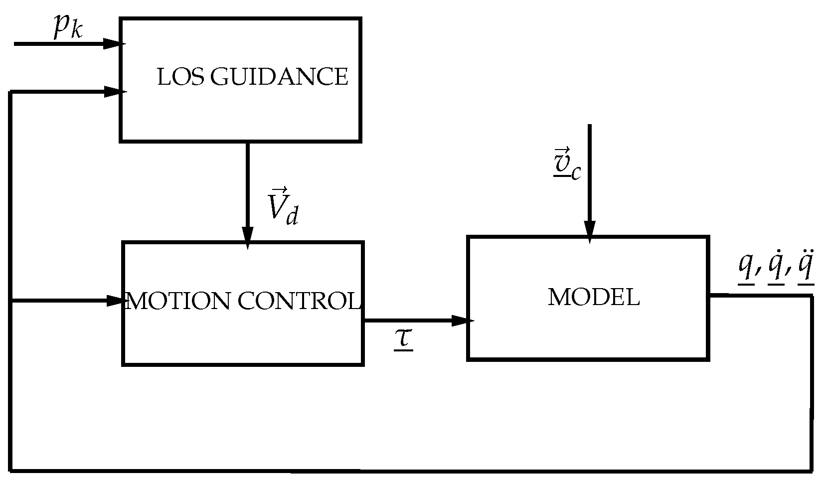
3. Design of The Controller

In this section, an adaptive sliding mode controller for the micro-AUV model subject to uncertainties and water currents is designed.

3.1. General Control Problem Formulation

Let us rewrite the equations of motion in the following general form for perturbed nonlinear systems:
x ¨ ( t ) = f ( x ˙ ( t ) , x ( t ) ) + g ( x ( t ) ) · u ( t ) + Δ ( t )
where Δ ( t ) represents the bounded perturbations such as model uncertainties and external disturbances. The equations of motion (25) computed in the previous section can be related to the formulation (32) by the following equalities:
x ( t ) = q ̲
u ( t ) = τ ̲
f ( x ˙ ( t ) , x ( t ) ) = M ̲ 1 H ̲ ( q ̲ , q ˙ ̲ )
g ( x ( t ) ) = M ̲ 1 S ̲ ( q ̲ )
The control objective here is defined as the desired velocity vector x ˙ d ( t ) in absolute coordinates computed from the desired speed vector in the body-fixed frame which is the real command input of the AUV. This command input can be given by the user directly (remote control) or by a trajectory controller (autonomous mode). The desired velocity vector in the body-fixed frame is defined as:
V d = [ u d , v d , w d , p d , q d , r d ] e ̲ 1
then one can compute this velocity vector in the reference frame:
x ˙ d ( t ) = q ˙ ̲ d = [ x d , y d , z d , p d , q d , r d ]
where
[ x d , y d , z d ] = [ u d , v d , w d ] A ̲ 10
Now that the desired velocities x ˙ d are computed, and so x ¨ d and x d , one can define the error vector e ( t ) characterizing the distance between the control objective and the command:
e ( t ) = x ( t ) x d ( t )
Then a sliding variable σ ( t ) 6 × 1 is defined as:
σ ( t ) = e ˙ ( t ) + λ e ( t )
with λ + * . By proposing a feedback linearizing controller, the vector u ( t ) is now defined as:
u ( t ) = g ( x ) 1 ( x ¨ d f ( x ˙ , x ) λ ( x ˙ x ˙ d ) + u a )
with g ( x ) non-singular. Using the classical notation from the dynamical model, u ( t ) is written as:
u ( t ) = S ̲ + M ̲ q ¨ ̲ + M ̲ 1 H ̲ λ ( q ˙ ̲ q ˙ ̲ d ) + u a
where u a 6 × 1 is called the auxiliary control vector. S ̲ + is the Moore-Penrose pseudo-inverse of S ̲ . The use of this algebraic tool is justified as the actuation matrix might not be squared and the system can be over or underactuated. The Moore-Penrose pseudo-inverse provides a least-square solution for u ( t ) to Equation (43) which is in the form S ̲ u = b .
Using the previous equations, one can define the closed-loop dynamics of the system using the derivative of the sliding variable σ :
σ ˙ = e ¨ + λ e ˙ = ( f ( x ˙ , x ) + g ( x ) · u + Δ x ¨ d ) + λ ( x ˙ x ˙ d )
By substituting (42) into (44), the σ dynamics are now given by:
σ ˙ ( t ) = u a ( t ) + Δ ( t )
The error dynamics are now driven by the auxiliary control variable u a regardless the nonlinearities of the system contained in the functions f and g.

3.2. Auxiliary Control and Disturbance Cancellation

The perturbations expected in the dynamics (internal or external) of the AUV can come from different sources: model estimation errors, measurement errors and external perturbations (oceanic currents for instance).
All these perturbations sources are synthesized into the bounded variable Δ ( t ) such that | Δ ( t ) | L 1 . With i [ 1 : 6 ] , one can define each term u a , i of the command vector using adaptive sliding mode control [26]:
u a , i ( t ) = K i , i ( t ) | σ i | 1 2 sign ( σ i ) K 2 i , i σ i
where K i , i and K 2 i , i are positive definite terms of the diagonal gain matrices K ( t ) and K 2 6 × 6 + . The adaptive law for K ( t ) is given for each of its diagonal terms K i , i with i [ 1 : 6 ] by:
K ˙ i , i ( t ) = k α , i sign ( | σ i | μ ) , if K i , i > K m i n , K m i n , if K i , i K m i n ,
with K m i n + * , k α , i + * and μ > 0 .
K m i n is the minimum adaptive gain, k α regulates the rate of adaptation, μ is a parameter detecting the loss of the sliding mode and thus increasing the gain if required. This particular controller adapts its gains to establish minimal control effort. Once the quasi-sliding mode is reached meaning that σ i < μ , the adaptive gain decreases to reduce the control constraints on the system.
This control method is robust against uncertain and disturbed systems, not overestimating control gain to reduce chattering. it allows the control to compensate the different sources of uncertainties and perturbations to reach and maintain the sliding mode i.e., | σ | < μ . Finally, the closed-loop dynamics can be written as:
σ ˙ i ( t ) = K i , i ( t ) | σ i ( t ) | 1 2 sign ( σ i ( t ) ) K 2 i , i σ i ( t ) + Δ i ( t )

3.3. Closed-Loop Stability

This subsection of the paper demonstrates the stability and finite-time convergence of the proposed control using Lyapunov direct method. The uncertain perturbation vector Δ ( t ) is bounded:
| Δ ( t ) | L 1 , L 1 > 0 .
The classical method is to select the Lyapunov candidate function:
V ( t ) = 1 2 σ 2 ( t )
with V ( 0 ) = 0 and V ( t ) > 0 for σ 0 . A sufficient condition to guarantee that the trajectory of the error translates from reaching phase to sliding phase is to choose the reaching condition such that:
V ˙ ( t ) = σ σ ˙ < η | σ | , σ 0 , η + *
If Equation (48) is substituted into (51) for each row i of the error vector, it gives:
V ˙ ( t ) = σ K ( t ) | σ | 1 / 2 sign ( σ ) K 2 σ + Δ ( t ) = | σ | K ( t ) | σ | 1 / 2 K 2 σ 2 + σ Δ ( t ) | σ | K ( t ) | σ | 1 / 2 K 2 σ 2 + | σ | L 1
Guaranteeing stability under the bounded perturbation Δ ( t ) implies the next statement to be respected:
| σ | K ( t ) | σ | 1 / 2 K 2 σ 2 + | σ | L 1 < η | σ | K ( t ) | σ | 1 / 2 + K 2 | σ | > L 1 + η
or the control signal being superior to the perturbation, which leads to the following constraint on the adaptive gain K a :
K ( t ) > 1 | σ | 1 / 2 L 1 + η K 2 | σ | K ( t ) > f c o n ( | σ | )
Three phases of the control sequence shall be analyzed to demonstrate the overall stability of the closed-loop dynamics. Let us consider the time t 0 where the controller initializes with the minimal adaptive gain K m i n and an initial error σ 0 such that | σ 0 | > μ . It exists a minimal gain K c o n that fulfills the constraint expressed in (54) and K c o n > K m i n . During this first phase, both K and | σ | increase. As the function f c o n ( | σ | ) is decreasing for | σ | increasing, there exists the time t 1 such that K ( t ) fulfills Equation (54). Thus, V ( t ) starts being monotonically decreasing from time t 1 and the system enters to phase 2.
During this next phase of the control, the system dynamics run under the following conditions:
σ σ ˙ < η | σ | , | σ | > μ
There exists an optimal gain K s m ( t ) > K c o n such that the virtual sliding mode surface is reached ( | σ | < μ ). Let us define the function V k ( t ) describing the internal convergence of the adaptive gain:
V k ( t ) = 1 2 K ˜ ( t ) 2
with K ˜ = K ( t ) K s m as the error estimation of optimal gain. Using the derivative of the function V k ( t ) , convergence can be analyzed:
V ˙ k ( t ) = K ˜ ( t ) K ˜ ˙ ( t ) = ( K ( t ) K s m ) k σ sign ( | σ | μ )
It is already established that K ( t ) < K s m , V ( t ) is decreasing and | σ | > μ . As a consequence, the following statements is written for phase 2:
V ˙ k ( t ) < κ | K ˜ | , κ + * V ˙ ( t ) < η | σ |
which means the global convergence of the adaptive gain K ( t ) is ensured by keeping both functions V ( t ) and V k ( t ) monotonically decreasing.
Using the previous assumptions, there exists the time t 2 defined by the achievement of the sliding mode such that | σ | μ and K ( t ) K s m . The system enters then to the third phase characterized by:
σ σ ˙ < η | σ | , | σ | < μ , K a ( t ) > K s m
These final conditions also ensure the global convergence of the function V k ( t ) by keeping its derivative V ˙ k ( t ) negative definite (statement (58) remains fulfilled). The adaptive gain K ( t ) then decreases until reaching the conditions of phase 2 (55). The global asymptotic convergence of both error variables σ ( t ) and K ˜ ( t ) is demonstrated.

4. Path-Following

In this section, a path-following controller is defined using the velocity control presented in Section 3. The objective for the AUV is to be able to follow autonomously a path defined by a series of waypoints. Each of these waypoints can be represented by a vector p k of this form:
w k = [ x p k , y p k , z p k , V p k ]
where x p k , y p k and z p k are the absolute coordinates of the waypoints in the NED frame. V p k is the desired norm of the AUV velocity vector (mostly surge and dive) at the considered waypoint (can be 0).
Let us define 2 consecutive waypoints p k and p k + 1 assuming the first one has already been passed and the AUV is heading toward the second one. Their coordinates are known and defined by:
r p k = [ x p k , y p k , z p k ] e ̲ 0
r p k + 1 = [ x p k + 1 , y p k + 1 , z p k + 1 ] e ̲ 0
as represented in Figure 3.
The unit vector characterizing the line between these 2 waypoints is defined by:
u k , k + 1 = r p k + 1 r p k | | r p k + 1 r p k | |
= [ u x , u y , u z ] e ̲ 0
Let us now introduce the principle of the Line Of Sight (LOS). It is a sphere of constant radius R whose center is the origin of the AUV body-fixed frame. If R is sufficiently large, there exist one or two intersection points between the sphere and the straight line defined by the 2 waypoints p k and p k + 1 . the vector between the AUV and the intersection point is the so-called LOS vector u L O S . The position of this intersection point is defined by the vector r L O S .
r L O S = [ x L O S , y L O S , z L O S ] e ̲ 0
To compute the LOS vector, one shall determine first the coordinates of r L O S . The equation of the R radius sphere centered in the AUV center of mass is the following expression:
( x L O S x ) 2 + ( y L O S y ) 2 + ( z L O S z ) 2 = R 2
The intersection point r L O S also belong to the line defined by the waypoints p k and p k + 1 . This leads to the following 3 equations:
x L O S = x p k + 1 + γ u x y L O S = y p k + 1 + γ u y z L O S = z p k + 1 + γ u z
To find the coordinates of the intersection between the LOS sphere and the path, one has to compute the variable γ by putting the equations of (67) into (66) which leads to the following second degree polynomial:
( x p k + 1 + γ u x x ) 2 + ( y p k + 1 + γ u y y ) 2 + ( z p k + 1 + γ u z z ) 2 R 2 = 0
γ 2 u x 2 + ( x p k + 1 x ) 2 + 2 γ u x ( x p k + 1 x ) + γ 2 u y 2 + ( y p k + 1 y ) 2 + 2 γ u y ( y p k + 1 y ) + γ 2 u z 2 + ( z p k + 1 z ) 2 + 2 γ u z ( z p k + 1 z ) R 2 = 0
The solutions for γ are of the form
γ 1 , 2 = β ± δ 2 α
with
α = u x 2 + u y 2 + u z 2 β = 2 u x ( x p k + 1 x ) + u y ( y p k + 1 y ) + u z ( z p k + 1 z ) δ = ( x p k + 1 x ) 2 + ( y p k + 1 y ) 2 + ( z p k + 1 z ) 2 R 2
Different situations can occur then:
  • δ < 0 which means no real solution for γ : there is no intersection between the sphere and the path. The LOS vector shall be defined as the vector from to the AUV position to p k + 1 .
  • γ 1 , 2 are both superior to 0: the LOS is ahead p k + 1 . The LOS vector shall also be defined as the vector from to the AUV position to p k + 1 .
  • γ 1 > 0 and γ 2 < 0 : γ 2 is the solution to compute the LOS vector.
  • γ 1 < 0 and γ 2 < 0 : γ 1 is the solution to compute the LOS vector (corresponds to the closest intersection point to p k + 1 ).
The computation of γ leads to the determination of the coordinates [ x L O S y L O S z L O S ] . The unit LOS vector is then:
u L O S = 1 R [ x L O S x , y L O S y , z L O S z ] e ̲ 0
= [ u L O S , x , u L O S , y , u L O S , z ] e ̲ 0
This result is then used to define the objective velocity vector for the vehicle in its body-fixed frame:
V o b j = V p k + 1 [ u L O S , x , u L O S , y , u L O S , z ] A ̲ 10 T e ̲ 1
= [ u o b j , v o b j , w o b j ] e ̲ 1
The desired forward and diving velocities, inputs to the controller defined in Section 3 are now:
[ u d , v d , w d ] = [ u o b j 2 + v o b j 2 , 0 , w o b j ]
Finally, the yaw angle error of the AUV e ψ is computed to control the desired yaw rate r d :
e ψ = a r c t a n v o b j u o b j
where the trigonometric function a r c t a n is defined as the 4-quadrant inverse tangent function. Then the desired yaw rate is expressed as it follows:
r d = K ψ e ψ
with K ψ a gain determined by the desired time response of the AUV for its yaw rate correction. Using (76) and (78), the complete desired velocity vector in the body-fixed frame is now defined:
V ̲ d = [ u d , 0 , w d , 0 , 0 , r d ] T
assuming that sway, roll and pitch velocities shall be maintained to 0 for this particular AUV control.
Figure 4 displays a diagram with the main components of the model and their respective major inputs and outputs to have a graphical overview of the system.

5. Numerical Simulations and Results

5.1. Numerical Parameters

This section provides first all the numerical values of the model parameters to simulate the underwater behavior of the AUV for different scenarios. In Table 1 are given the main parameters values of the AUV.
The linear damping parameters are estimated using SolidWorks Flow Simulation (Dassault Systèmes SolidWorks Corporation - Waltham, Massachusetts - USA) for various water flow speeds on the micro-AUV prototype model (see Figure 1). Added masses and inertia, as rotational damping parameters are estimated using several data from other references about AUVs approximately of the same size and shape.
To simulate uncertainties in the model dynamics, all the parameters in Table 1 have been increased or decreased arbitrarily by 15% while the nominal parameters have been kept to compute the control signal u ( t ) from Equation (43).
In Table 2 are given the different parameter values for the proposed adaptive sliding mode controller. These values are arbitrary and have been chosen for the controller to have suitable dynamics regarding the application. K 2 and K m i n define the minimum control effort desired and null values are prohibited to avoid instability. μ is the threshold on the sliding variable to avoid excessive control effort for maintaining the system on the sliding surface. K α is the main parameter and drives the rate of adaptation. If the value is too small, the system could not be able to compensate for the different perturbations and become unstable. At the opposite, an excessive value would increase the chattering level and require non-feasible control dynamics from the actuators.

5.2. Results

In this section, the dynamical model (29) behavior in closed-loop with the control (43) and (46) is evaluated using Matlab/Simulink with a Runge–Kutta solver at sampling frequency of 1 k H z . For the sake of simplicity, it is assumed that the full state vector is available. Three scenarios are investigated to apprehend the micro-AUV behavior under various conditions:
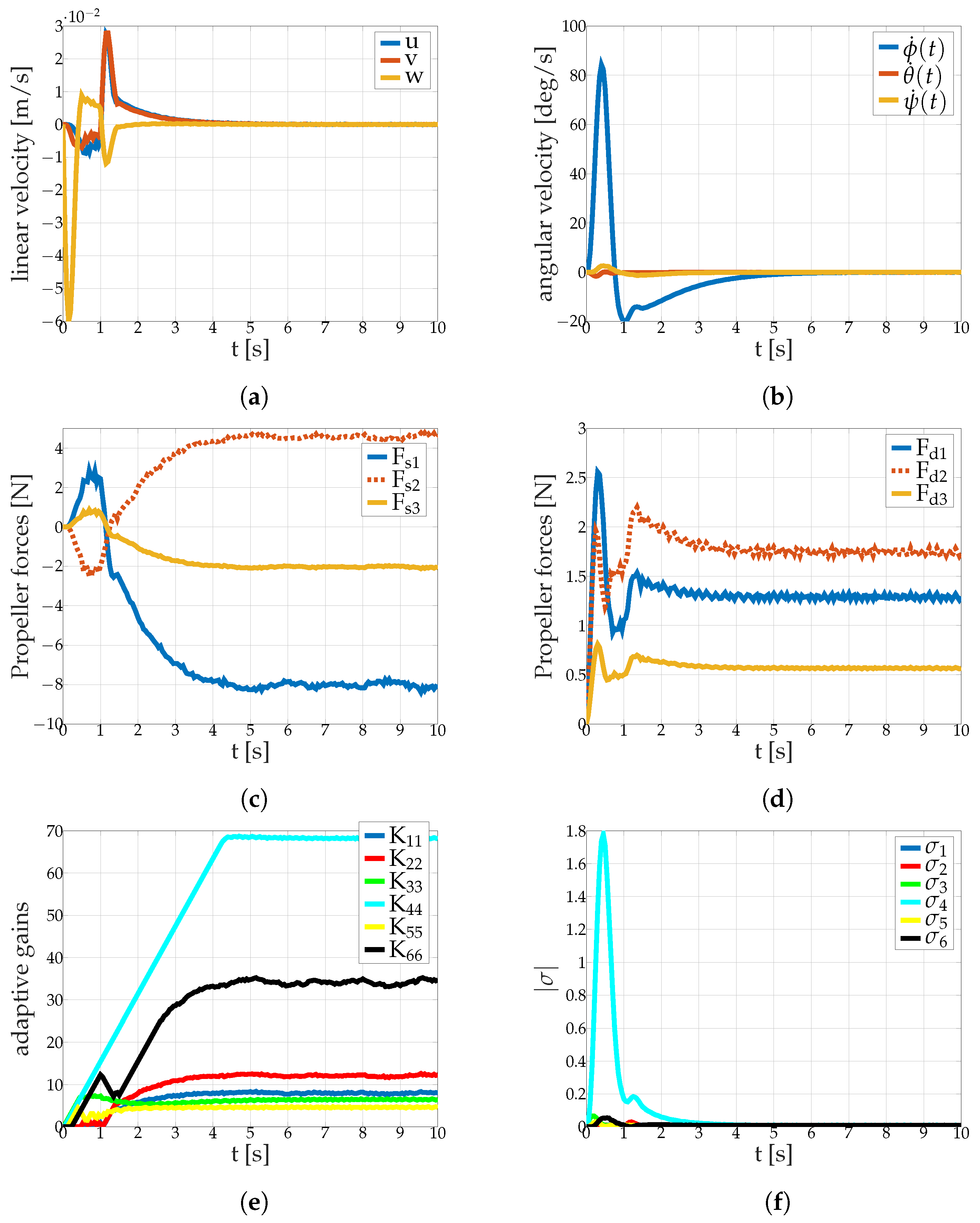
  • Step response to a velocity command with and without internal and external perturbations
  • The AUV remains in steady state under perturbations
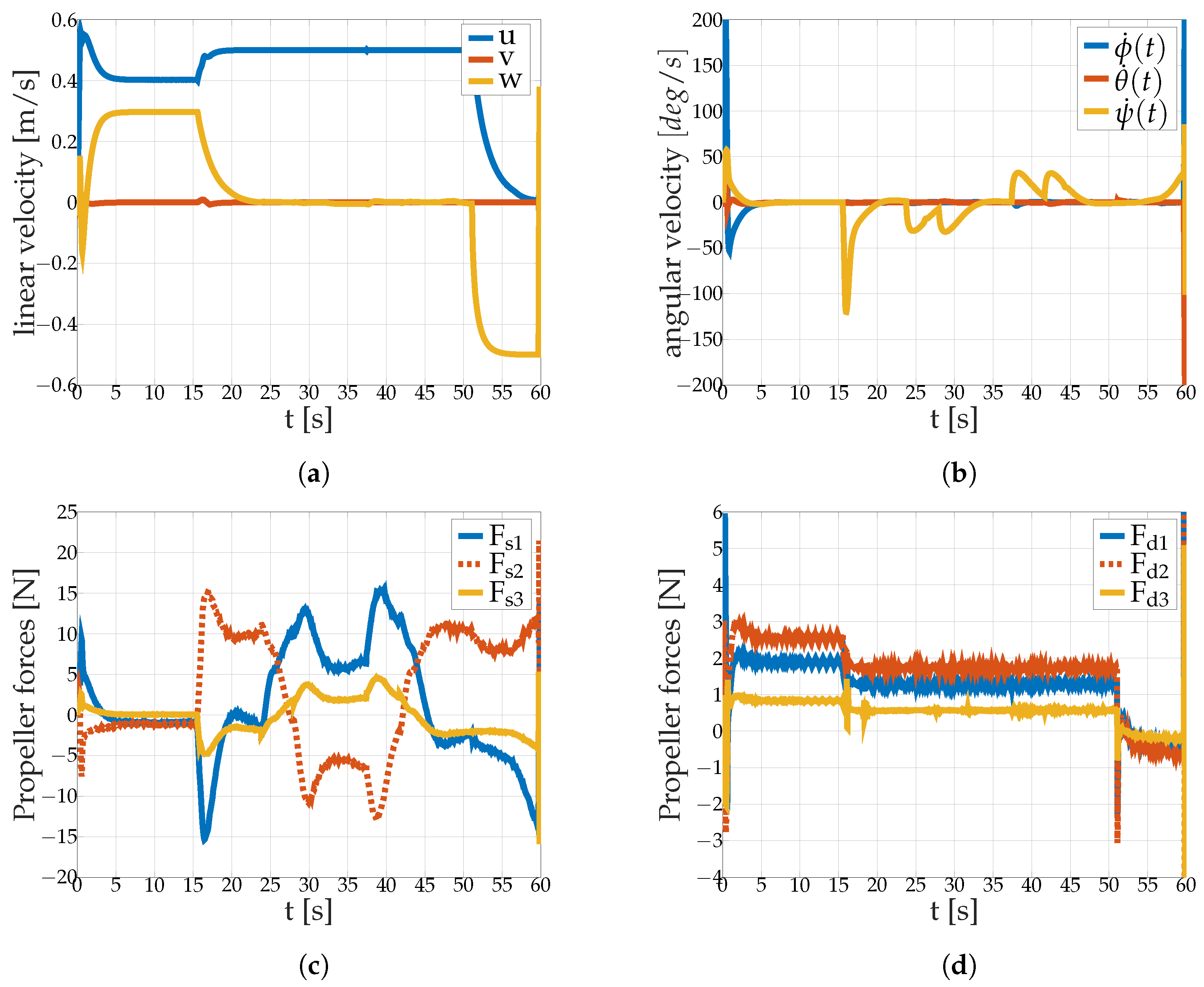
  • The AUV follows a defined path under perturbations

5.2.1. Surge Velocity Control Avoiding Sideslip

The objective of this simple maneuver is to demonstrate the ability of the controller to maintain a constant forward speed u of 1 m . s 1 without sway or yaw velocity deviation (v and ψ ˙ shall remain 0) and at constant depth. This maneuver is performed with and without model uncertainties or ocean current to observe the adaptive controller compensation behavior. The initial conditions of the AUV are q ̲ = q ̲ ˙ = q ̲ ¨ = 0 ̲ .
In Figure 5 are plotted the results from the first scenario without any internal or external disturbance. One shall notice that some variables might appear on the legend but not on the graph because of their null value. Figure 5a displays the AUV velocities in its body-fixed frame. In a first time occurs the transient response of the system where the controller receives an error information from the sliding variable σ (see Figure 5d) an begin to compensate with the actuators (thruster forces in Figure 5c. One can observe at this first time interval t [ 0 0.6 ] s the term K 11 (see Figure 5b) increasing from K m i n to 4.7 until the sliding variable σ reaches the threshold μ of 1.10 2 . Then, in absence of perturbation ( | Δ ( t ) | = 0 t ), the time derivative of the adaptive gain K 11 becomes negative and its value decreases to K m i n as long as the error σ remains inferior to the threshold μ . Finally, the control succeeds in maintaining the AUV at a constant forward speed u = 1 m·s 1 while its other linear and angular velocities remain zero.
In Figure 6 are plotted the results from the first scenario with model parametric uncertainties and water current as an external disturbance. Figure 6a displays the AUV linear velocities in its body-fixed frame. One can observe that the final velocity behavior of the AUV remains almost equal to the previous simulation. However, the controller reacts differently when facing the water current. In the Figure 6e, the two adaptive gains K 11 and K 22 (water current in the ( x y ) plane) increase their value until σ converges to sliding mode (Figure 6f). As the main difference with the previous case, the adaptive gains reach stabilized values corresponding to the cancellation of the current effect. These new values lead to a new equilibrium of thrust forces plotted in Figure 6c,d. Thus, the adaptive control succeeds in maintaining the AUV at a constant forward speed u = 1 m/s and shows robustness against perturbations.
The Figure 7 presents the comparison of the two trajectories (with and without perturbation). One can see the trajectory deviation of the AUV in the ( x y ) plane is around 2.10 1 m. This error is because the control is based on a desired velocity vector, not positions with respect to time.

5.2.2. Steady State stabilization

The objective of this scenario is to observe the position deviation and the control behavior while unexpected water current hits suddenly the micro-AUV performing a fixed position task such as seafloor object manipulation or submerged pipes maintenance. Moreover, the AUV model is also subject to parametric uncertainties.
In the Figure 8 are plotted the results from scenario 2. One can observe the transient phenomenon occurring at time t = 1 s on each graph. Figure 8a shows that the linear velocities of the AUV are affected by the sudden perturbation between for t [ 1 5 ] s. At t = 5 s, the system succeeds in maintaining a steady state position given the perturbation (see the error value of σ in Figure 8f). Figure 8c,d display the propeller forces equilibrium, very similar to Figure 6c,d as the system is dealing with the same perturbation. The Figure 9 displays the ( x y ) plane displacement of the AUV during the maneuver. As in the previous scenario, the final position error is about 1·10 2 m in each direction.

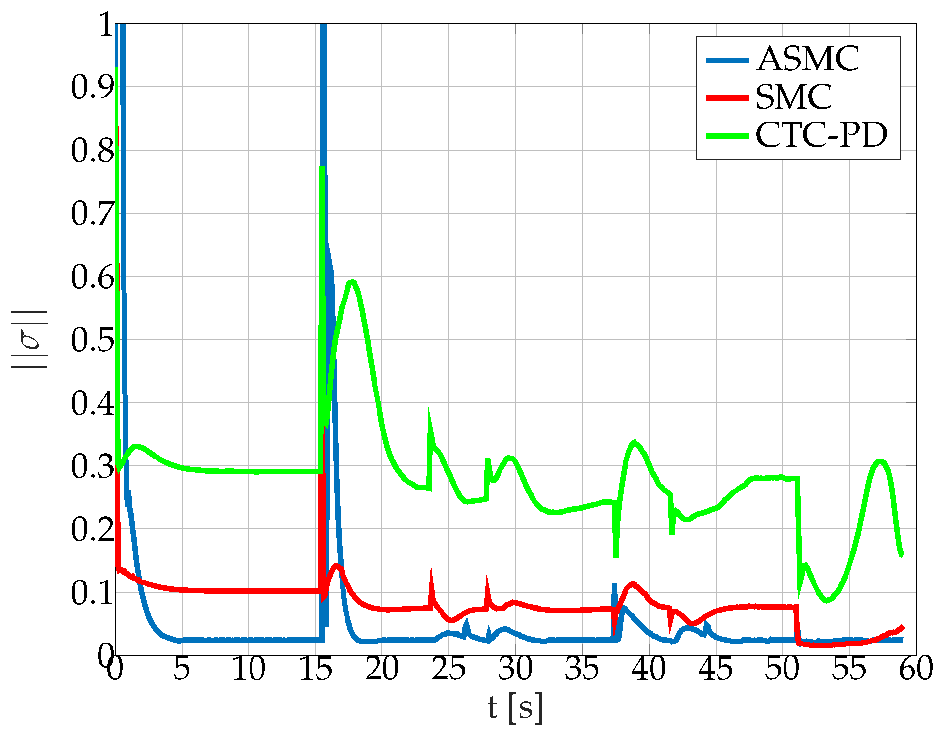
5.2.3. Path-Following Task

The objective of this last maneuver is to observe the adaptive control (low-level control) working with the path-following algorithm (high-level control) to perform a waypoints route following task of 60 s at a constant speed of 0.5 m·s 1 . Model parametric uncertainties and external perturbation are also added to the simulation.
In the Figure 10 are plotted the results from scenario 3. The linear and angular velocities of the AUV are shown in Figure 10a,b. One can observe that the total norm of the velocity vector remains constant (0.5 m·s 1 ) during the whole maneuver. The different transient phases in the angular velocity correspond to the AUV heading changes when passing a waypoint.
In Figure 11 and Figure 12 are plotted the adaptive gains and the corresponding error variables σ . It is easy to notice that the adaptive control is constantly compensating the perturbation, especially during the heading changes as the water current relative direction with respect to the AUV body-fixed frame changes (see the gains K 1 , 1 and K 2 , 2 , in blue and red associated with the degrees of freedom x and y). Furthermore, the gain K 3 , 3 (z degree of freedom) adapts during the three phases when diving velocity is required to change.
In Figure 10c,d are also plotted the forces from the two propellers groups: surge/sway/yaw and dive/roll/pitch.
Figure 13 displays the trajectory of the underwater vehicle for the three tested controllers. The proposed adaptive control succeeds in maintaining the AUV on a defined path at a constant speed while dealing with a variable direction perturbation.
The three different proposed simulation scenarios illustrated the efficiency of the control to deal with high parametric uncertainties (15%) and an external realistic perturbation. These properties are essential especially for a micro-AUV compared with heavier models. Indeed, for larger AUVs the relative model uncertainties and the impact of water current shall be significantly lower.
Finally, the results of the proposed ASMC are compared with other two control methods on the path-following task. From the expression (46), two other controllers are derived:
S M C : K i , i = 25 , K 2 i , i = 1
P D : K i , i = 0 , K 2 i , i = 30
Figure 14 and Figure 15 respectively display the norm of the control signal and the norm of the sliding variable vector for the three controllers. The proposed ASMC control exhibits few differences in the control signal compared to the other controllers, manages to significantly reduce the error σ . Moreover, the adaptation law allows decreasing the chattering phenomenon compared with SMC.
These observations are synthesized into numerical indicators in Table 3. With approximately the same amount of control energy, the error signal energy and the chattering indicator represented by the Kurtosis of the control signal are inferior for the proposed ASMC controller in comparison with the two other control methods.

6. Conclusions

An adaptive sliding mode control for a micro autonomous underwater vehicle to reject bounded perturbations has been designed, where the finite-time convergence demonstration using the Lyapunov method was provided. The proposed control allowed achieving low-level tasks such as velocity control and regulation as well as high levels tasks such as autonomous path-following using waypoints. Each task has been successfully performed in the presence of realistic perturbations such as a random irrotational water current and model parametric uncertainties. To provide a detailed and realistic testing environment, a model using the Lagrange approach was developed, in contrast with the standard Newton-Euler method. The model included underwater effects such as added mass and inertia, hydrodynamic damping and buoyancy. Simulation results demonstrated that the proposed adaptive control, compared with other standard control methods, has better precision and robustness and so is deeply relevant for this particular kind of application.

Author Contributions

Conceptualization, Methodology, Formal analysis J.R. and H.C.; Writing—Original Draft Preparation J.R.; Writing—Review and Editing H.C. and J.L.G.

Funding

This research received no external funding.

Conflicts of Interest

The authors declare no conflict of interest.

References

  1. Zereik, E.; Bibuli, M.; Mišković, N.; Ridao, P.; Pascoal, A. Challenges and future trends in marine robotics. Annu. Rev. Control 2018, 46, 350–368. [Google Scholar] [CrossRef]
  2. Roberts, G.N.; Sutton, R. Advances in Unmanned Marine Vehicles; Book IEEE Control Series; IEEE: Piscataway, NJ, USA, 2006; pp. 13–42. [Google Scholar]
  3. García-Valdovinos, L.G.; Salgado-Jiménez, T.; Bandala-Sánchez, M.; Nava-Balanzar, L.; Hernández-Alvarado, R.; Cruz-Ledesma, J.A. Modelling, Design and Robust Control of a Remotely Operated Underwater Vehicle. Int. J. Adv. Robot. Syst. 2014, 11, 1. [Google Scholar] [CrossRef] [Green Version]
  4. De Souza, E.C.; Maruyama, N. Intelligent UUVs: Some Issues on ROV Dynamic Positioning. IEEE Trans. Aerosp. Electron. Syst. 2007, 43, 214–226. [Google Scholar] [CrossRef]
  5. Christ, R.D.; Wernli, R.L., Sr. The ROV Manual: A User Guide for Remotely Operated Vehicles, 2nd ed.; Elsevier: Amsterdam, The Netherlands, 2014; pp. 14–31. [Google Scholar]
  6. Fossen, T.I. Handbook of Marine Craft Hydrodynamics And Motion Control, 1st ed.; Wiley: Hoboken, NJ, USA, 2011; Volume 167–186, pp. 241–284. [Google Scholar]
  7. Fossen, T.I. Marine Control Systems. Guidance, Navigation and Control of Ships, Rigs and Underwater Vehicles; Marine Cybernectics AS: Trondheim, Norway, 2002; pp. 88–103. [Google Scholar]
  8. Antonelli, G.; Chiaverini, S.; Sarkar, N.; West, M. Adaptive Control of an Autonomous Underwater Vehicle: Experimental Results on ODIN. IEEE Trans. Control Syst. Technol. 2001, 9, 756–765. [Google Scholar] [CrossRef]
  9. Chen, C.W.; Kouh, J.S.; Tsai, J.F. Modeling and Simulation of an AUV Simulator with Guidance System. IEEE J. Ocean. Eng. 2013, 38, 211–225. [Google Scholar] [CrossRef]
  10. Ribas, D.; Palomeras, N.; Ridao, P.; Carreras, M.; Mallios, A. Girona 500 AUV: From Survey to Intervention. IEEE/ASME Trans. Mechatron. 2012, 17, 46–53. [Google Scholar] [CrossRef]
  11. Carreras, M.; Hernández, J.D.; Vidal, E.; Palomeras, N.; Ribas, D.; Ridao, P. Sparus II AUV—A Hovering Vehicle for Seabed Inspection. IEEE J. Ocean. Eng. 2018, 43, 344–355. [Google Scholar] [CrossRef]
  12. Jalving, B. The NDRE-AUV Flight Control System. IEEE J. Ocean. Eng. 1994, 19, 497–501. [Google Scholar] [CrossRef]
  13. Naeem, W.; Sutton, R.; Ahmad, S.M. LQG/LTR Control of an Autonomous Underwater Vehicle Using a Hybrid Guidance Law. Int. Fed. Autom. Control J. 2003, 36, 31–36. [Google Scholar] [CrossRef]
  14. Fjellstad, O.-E.; Fossen, T.I. Position and Attitude Tracking of AUVs: A Quaternion Feedback Approach. IEEE J. Ocean. Eng. 1994, 19, 512–518. [Google Scholar] [CrossRef]
  15. Cui, R.; Chen, L.; Yang, C.; Chen, M. Extended State Observer-Based Integral Sliding Mode Control for an Underwater Robot With Unknown Disturbances and Uncertain Nonlinearities. IEEE Trans. Ind. Electron. 2017, 64, 6785–6795. [Google Scholar] [CrossRef] [Green Version]
  16. Chin, C.S.; Lin, W.P. Robust Genetic Algorithm and Fuzzy Inference Mechanism Embedded in a Sliding-Mode Controller for an Uncertain Underwater Robot. IEEE/ASME Trans. Mechatron. 2018, 23, 655–666. [Google Scholar] [CrossRef]
  17. Fossen, T.I.; Sagatun, S. Adaptive control of nonlinear systems: A Case Study of Underwater Robotics Systems. J. Robot. Syst. 1991, 8, 393–412. [Google Scholar] [CrossRef]
  18. Refsnes, J.E.; Sørensen, A.J.; Pettersen, K.Y. Model-Based Output Feedback Control of Slender-Body Underactuated AUVs: Theory and Experiments. IEEE Trans. Control Syst. Technol. 2008, 15, 930–946. [Google Scholar] [CrossRef]
  19. Antonelli, G. On the Use of Adaptive/Integral Actions for Six-Degrees-of-Freedom Control of Autonomous Underwater Vehicles. IEEE J. Ocean. Eng. 2007, 32, 300–312. [Google Scholar] [CrossRef]
  20. Savaresi, S.M.; Previdi, F.; Dester, A.; Bittanti, S.; Ruggeri, A. Modeling, Identification, and Analysis of Limit-Cycling Pitch and Heave Dynamics in an ROV. IEEE J. Ocean. Eng. 2004, 29, 407–417. [Google Scholar] [CrossRef]
  21. Soylu, S.; Proctor, A.A.; Podhorodeski, R.P.; Bradley, C.; Buckham, B.J. Precise Trajectory Control for an Inspection Class ROV. Ocean Eng. 2016, 111, 508–523. [Google Scholar] [CrossRef]
  22. Lapierre, L.; Jouvencel, B. Robust Nonlinear Path-Following Control of an AUV. IEEE J. Ocean. Eng. 2008, 33, 89–102. [Google Scholar] [CrossRef]
  23. Cui, R.; Zhang, X.; Cui, D. Adaptive Sliding Mode Attitude Control for Autonomous Underwater Vehicles with Input Nonlinearities. Ocean Eng. 2016, 123, 45–54. [Google Scholar] [CrossRef]
  24. Qiao, L.; Zhang, W. Adaptive non-singular integral terminal sliding mode tracking control for autonomous underwater vehicles. IET Control Theory Appl. 2017, 11, 1293–1306. [Google Scholar] [CrossRef]
  25. Guerrero, J.; Torres, J.; Creuze, V.; Chemori, A. Trajectory Tracking for Autonomous Underwater Vehicle: An adaptive Approach. Ocean Eng. 2019, 172, 511–522. [Google Scholar] [CrossRef] [Green Version]
  26. Shtessel, Y.; Edwards, C.; Fridman, L.; Levant, A. Sliding Mode Control and Observation; Springer: New York, NY, USA, 2014. [Google Scholar]
Figure 1. AUV model: frames definitions.
Jmse 07 00445 g001
Figure 2. AUV model: joint vectors configuration.
Jmse 07 00445 g002
Figure 3. LOS guidance schematic representation in the ( x y ) plane.
Jmse 07 00445 g003
Figure 4. Model, control and navigation diagram.
Jmse 07 00445 g004
Figure 5. 1 m/s surge speed command (without disturbance): (a) AUV linear velocities (b) adaptive control gains (c) adaptive propeller forces (d) sliding variable vector σ absolute value.
Jmse 07 00445 g005
Figure 6. 1 m/s surge speed command (with disturbance): (a) AUV linear velocities (b) AUV angular velocities (c) horizontal propellers forces (d) vertical propellers forces (e) adaptive control gains (f) sliding variable vector σ absolute value.
Jmse 07 00445 g006aJmse 07 00445 g006b
Figure 7. 1 m/s surge speed command: 3D trajectory of the AUV.
Jmse 07 00445 g007
Figure 8. Steady state command (sudden oceanic current at t = 1 s): (a) AUV linear velocities (b) AUV angular velocities (c) horizontal propellers forces (d) vertical propellers forces (e) adaptive control gains (f) sliding variable vector σ absolute value.
Jmse 07 00445 g008
Figure 9. Steady state command (sudden oceanic current at t=1s): ( x y ) plane trajectory of the AUV.
Jmse 07 00445 g009
Figure 10. Path-following task: (a) AUV linear velocities (b) AUV rotational velocities (c) Surge/Sway propeller forces (d) Dive propeller forces.
Jmse 07 00445 g010
Figure 11. Path-following task: adaptive gains.
Jmse 07 00445 g011
Figure 12. Path-following task: sliding variable vector σ absolute value.
Jmse 07 00445 g012
Figure 13. Path-following task: 3D trajectory of the AUV.
Jmse 07 00445 g013
Figure 14. Path-following task: norm of the control signal u, comparison of the 3 controllers.
Jmse 07 00445 g014
Figure 15. Path-following task: norm of the sliding variable vector σ , comparison of the 3 controllers.
Jmse 07 00445 g015
Table 1. AUV model: glossary and numerical data.
VariableDescriptionValueUnit
m 1 AUV mass 2.5 [kg]
m a x x-axis added mass 0.36 × m 1 [kg]
m a y y-axis added mass 1 × m 1 [kg]
m a z z-axis added mass 1.15 × m 1 [kg]
J x x roll inertia 0.0049 [kg·m 2 ]
J y y pitch inertia 0.023 [kg·m 2 ]
J z z yaw inertia 0.0021 [kg·m 2 ]
J x x a added roll inertia 0.36 × 0.0049 [kg·m 2 ]
J y y a added pitch inertia 1 × 0.023 [kg·m 2 ]
J z z a added yaw inertia 1.15 × 0.0021 [kg·m 2 ]
r ̲ B / C M 0 T Buoyancy[0 0 0][m]
b ̲ s 1 0 T propeller position[0.06 0.126 0][m]
b ̲ s 2 0 T propeller position[0.06 −0.126 0][m]
b ̲ s 3 0 T propeller position[−0.28 0 0][m]
b ̲ d 1 0 T propeller position[0.03 0.1 0][m]
b ̲ d 2 0 T propeller position[0.03 −0.1 0][m]
b ̲ d 3 0 T propeller position[−0.19 0 0][m]
α 1 propeller orientation−40/180· π [rad]
α 2 propeller orientation40/180· π [rad]
α 3 propeller orientation π / 2 [rad]
ρ water density1000[kg·m 3 ]
ggravity 9.81 [m·s 2 ]
Vdry volume 2.58 × 10 3 [m 3 ]
X | u | u quadratic damping5.85[N·m 2 ·s 2 ]
X u quadratic damping0.048[N·m·s 1 ]
Y | v | v quadratic damping11.98[N·m 2 ·s 2 ]
Y v quadratic damping0[N·m·s 1 ]
Z | w | w quadratic damping21.85[N·m 2 ·s 2 ]
Z w quadratic damping0.044[N·m·s 1 ]
K | p | p quadratic damping5.85[N·m 2 ·s 2 ]
K p quadratic damping0[N·m·s 1 ]
M | q | q quadratic damping11.98[N·m 2 ·s 2 ]
M q quadratic damping0[N·m·s 1 ]
N | r | r quadratic damping21.85[N·m 2 ·s 2 ]
N r quadratic damping0[N·m·s 1 ]
RLOS radius1[m]
μ c current parameter1 [ ]
w m e a n average1 [ ]
w s t d standard deviation0.5 [ ]
v ̲ c current velocity vector [ 110 ] V c e ̲ 0 [m·s 1 ]
Table 2. AUV model: Control parameters.
VariableValue
K m i n 1.10 2
K 2 1
K α 16
λ 1
μ 1.10 2
Table 3. Path-following task: numerical indicators for comparison of the 3 controllers.
ASMCSMCCTC-PD
0 t e n d | | u | | 5.67 × 10 8 5.58 × 10 8 5.4 × 10 8
0 t e n d | | σ | | 4 × 10 6 4.83 × 10 6 16.7 × 10 6
K u r t o s i s ( u ) 3.01 10.87 5.03

