Article

Response of a Porous Seabed around an Immersed Tunnel under Wave Loading: Meshfree Model

1
School of Engineering and Built Environment, Griffith University Gold Coast Campus, Queensland 4222, Australia
2
Department of Marine Environmental Engineering, National Kaohsiung University of Science and Technology, Kaohsiung 80778, Taiwan
3
Department of Marine Environment and Engineering, National Sun Yat-Sen University, Kaohsiung 80424, Taiwan
4
Center of Excellence for Ocean Engineering, National Taiwan Ocean University, Keelung 20224, Taiwan
*
Author to whom correspondence should be addressed.
These authors contributed equally to this work.
J. Mar. Sci. Eng. 2019, 7(10), 369; https://doi.org/10.3390/jmse7100369
Submission received: 22 August 2019 / Revised: 11 October 2019 / Accepted: 12 October 2019 / Published: 17 October 2019
(This article belongs to the Special Issue New Advances in Marine Engineering Geology)

Abstract

:
Seabed instability surrounding an immersed tunnel is a vital engineering issue regarding the design and maintenance for submarine tunnel projects. In this study, a numerical model based on the local radial basis function collocation method (LRBFCM) is developed to evaluate the seabed behaviour in a marine environment, in which the seabed is treated as the porous medium and governed by Biot’s “ u p ” approximation. As for the flow field above the seabed, the VARANS equations are used to simulate the fluid motion and properties. The present model is validated with analytical solutions and experimental data which show a good capacity of the integrated model. Both wave and current loading are considered in this study. Parametric studies are carried out to investigate the effects of wave characteristics and soil properties. Based on the numerical results, the maximum liquefaction depth around the immersed tunnel could be deeper under the wave loading with long wave period (T) and large wave height (H). Moreover, a seabed with lower permeability ( K s ) and degree of saturation ( S r ) is more likely to be liquefied.

1. Introduction

In recent years, to meet the continual improvement requirements in coastal transportation, the immersed tunnel has become one of the choices to fundamentally transform the transport in the region of oceans and rivers, replacing the conventional methods such as the ferry. The immersed tunnel has a history of about 100 years and it shows a good performance in reliability and applicability under complex natural dynamic loading; for example, the longest immersed tunnel in the world, the Hongkong–Zhuhai–Macao Bridge immersed tunnel. As an alternative to a bridge, the immersed tunnel has advantages in less environmental effects and no obstruction of navigation channels. Compared to bridges, the immersed tunnel is commonly constructed in a soft and loose seabed. Thus, the stability of the seabed soil surrounding the immersed tunnel in complex marine environments becomes one of the main concerns implicated in tunnel design and maintenance.
It has been recognized that the pore water pressures and stresses in seabeds are affected by the water pressures generated by the natural dynamic loading. If the pore water pressure reaches the limit value, the liquefaction could occur with the effective stress in seabed vanishing. To avoid seabed instability around the immersed tunnel, the study of seabed dynamic behaviour is necessary under the real hydrodynamic loading. Two mechanisms of wave-induced liquefaction has been figured out based on a mass of laboratory tests and field exploration [1,2,3], which are transient liquefaction and residual liquefaction. The transient liquefaction is motivated by the oscillatory excess pore water pressures under wave pressure vibration which usually happens with amplitude reduction and phase lag of pore pressure in seabed soil [4]. While the residual liquefaction is on the consequence of the excess pore water pressure build-up under cyclic wave loading [5]. Later, Jeng and Seymour [6] proposed a simplified approximation to predict the liquefaction process in a large seabed, and concluded that the residual mechanism is more essential under large waves while the transient mechanism is dominate in a seabed under small wave loading.
In the past 40 years, various analytical formulas have been developed and verified in regard to the seabed dynamic response [4,7,8]. However, the seabed dynamic response around the structure is difficult to be described by analytical methods. Thus, several numerical model was developed to simulate the soil behaviour around the offshore structures, such as breakwaters [9], and buried pipes [10]. However, the research of a wave-induced response around the undersea immersed tunnel is quite limited. For instance, a real case simulation of the Busan–Geoje fixed link in South Korea was conducted by Kasper et al. [11] under large waves (wave height up to 9.2 m) generated by typhoons. Nevertheless, this study did not consider the impact of the seabed liquefaction around the tunnel. Recently, [12,13] simulated the seabed transient and residual response around the immersed tunnel under wave loading based on Biot’s consolidation equations neglecting the inertial terms for soil skeleton and fluid phase.
In natural ocean environments, current is another crucial component besides wave. For instance, a long-term mentoring data of the Lingding Bay, in which the Hong Kong–Zhuhai–Macau bridge tunnel located, shows the current co-exists with wave varying from bottom to surface as the consequence of the irregular semi-diurnal tide. The maximum velocity of the surface current reaches up to 1.5 m/s [14]. The interaction between current and wave is found to be able to affect the hydrodynamic properties directly and further impact the porous seabed dynamics. Ye and Jeng [15] investigated the transient response of a porous seabed under wave combined current loading firstly. Later, the current effects in the vicinity of a submarine pipeline were examined by Wen et al. [16] based on the commercial software ABAQUS. Lately, Liao et al. [17] simulated the residual seabed liquefaction under the flow field that wave and current generated simultaneously. To date, how current affect the liquefaction of seabed soil surrounding the immersed tunnel has not been examined yet to the author’s knowledge.
The aforementioned numerical models mainly developed adopting the conventional methods such as the finite element method and finite difference method. In recent years, a new numerical technique has come up which uses a set of nodes instead of the conservative meshes to approximate the solution. In consequence of discretization of the partial differential equations directly on nodes instead of meshes, the meshfree method is more qualified in dealing with mesh entanglement problems and constructing the approximations with arbitrary order of continuity than the traditional mash-based numerical methods. The start point of the meshfree method was using the moving least-square (MLS) method to establish shape functions for a set of scatter nodes by Nayroles et al. [18]. After that, Belytschko et al. [19] used the Galerkin weak form to improve the diffuse element method, which formed a new element-free Galerkin method. The element-free Galerkin method has been widely used in soil mechanics problems. In addition, an innovative interpolation scheme to overcome the disadvantage of the MLS was proposed by Liu and Gu [20], which is called the point interpolation method (PIM). The original PIM method picks up the polynomial basis as the basis function which performs well for one dimensional problems. However, it is hard to determine the ranks when this method extended to multi-dimensional range, which is the result of basis function selection. In order to figure this problem, Wang et al. [21] proposed a point interpolation method based on the radial basis functions (RBF). This method maps the multi-dimensional space into one-dimensional space though a radial function, which makes choosing basis function easier. This method has been widely used on the geomechanics problems. For example, Wang and Liu [22] simulated the Biot’s consolidation process by radial PIM method. The displacement and the pore water pressure were discretised by the same shape function in space, while the fully implicit integration scheme was adopted for time discretization to avoid the spurious ripple effect. In the literatures, two different type of the RBFs are commonly used, which are the multiquadrics (MQ) [23], and the Gaussian radial basis functions [24]. In this study, the MQ was used. These functions were first under intensive research in multivariate data interpolation and used to solve the partial differential equations by Kansa [25]. Thus, this method is usually called Kansa’s method, and is known as the global RBF collocation method (GRBFCM). This method has been applied to computational fluid dynamics problems such as solutions of the Navier–Stokes equation [26], natural convections in porous media [27], numerical wave tanks [28], and solid–liquid phase change problems [29]. The GRBFCM has the obvious advantages in dealing with arbitrary and complex domain, which applied in many field, such as surface fitting, turbulence analysis, neural networks, meteorology. However, ill-conditions can occur when the resolution is high. For the purpose of overcoming the difficulties of ill-conditions as mentioned above, a localization procedure to transform the dense matrices into sparse matrices was proposed. On the basis of the multiquadric RBF [30], Lee et al. [31] proposed the local RBF collocation method (LRBFCM) for the first time. This method has been applied in various fields, such as the solutions of diffusion problem [32], Darcy flow in porous media [33], water wave scattering [34], macro-segregation phenomena [35] and so on. Recently, Wang et al. [36] adopted the LRBFCM based on the Biot’s consolidation equation to simulate a wave-induced seabed response around a pipeline.
In this paper, an integrated numerical model is proposed to simulate the sandy seabed dynamic response and transient liquefaction in the vicinity of an immersed tunnel under natural complex loading. The flow model is developed based on IHFOAM [37], while the seabed model is established adopting the LRBFCM with Biot’s “ u p ” approximation which considered the inertial term of soil skeleton. The verification of the integrated model is carried out by comparisons with the analytical solution [7] and published experimental data [38]. In this study, the effects of the current on the seabed behaviour around the immersed tunnel are examined. Parametric studies are conducted in regard of the different wave characteristics and soil properties.

2. Theoretical Models

In this study, an integrated 2D numerical model is developed to simulate the fluid-structure seabed interaction, which is composed of two sub-models: the flow model and seabed model. The flow model is responsible for simulating the wave motion including the wave pressure and current velocity, while the seabed model evaluates the effective stress, displacement, and pore pressure in the seabed under the dynamic loading. The two sub-models adopt the one-way coupling algorithm which is connected by the continuous water pressure.

2.1. Flow Model

In this paper, the flow model is based on one of the solvers in OpenFOAM®, IHFOAM. Recently, some other open-source codes have been developed for modeling wave propagation and wave–structure interaction problems [39,40] as well. To simulate the coastal, offshore, and hydraulic engineering process, this model solves the three-dimensional Volume Averaged Reynolds Averaged Navier–Stokes (VARANS) equations with regard to two incompressible phases of air and water. The fluid model adopts the finite volume discretization and the volume of fluid (VOF) method [37]. Including continuity and momentum conservation equations; the VARANS equations as the governing mathematical expressions in this model can be expressed as:
u i x i = 0 ,
ρ f u i t + x j 1 n ρ f u i u j = n p f x i + n ρ f g i + x j μ e f f u i x j [ C T ] ,
where is Darcy’s volume averaging operator, while f is the intrinsic averaging operator; ρ f represents the density which is computed by ρ f = α ρ w a t e r + ( 1 α ) ρ a i r ; α is the indicator function defined in (5); u i is the velocity vector while n is the porosity; p is the pseudo-dynamic pressures; g , g i is the gravitational acceleration; μ e f f is the efficient dynamic viscosity, defined as μ e f f = μ + ρ f ν t u r b , in which μ is the molecular dynamic viscosity and ν t u r b is the turbulent kinetic viscosity, given by the chosen turbulence model. The k ϵ turbulence model is adopted in this study; the last term in (2) corresponds to the resistance of porous media, which is shown as:
[ C T ] = A u i + B | u | u i + C u i t ,
compared to factors A and B, factor C is less significant. Moreover, 0.34 (kg/m 3 ) is often adopted for the value of C by default [41].
In present fluid model, the values of A and B are derived by Engelund [42]’s formulae, which also employed in Burcharth and Andersen [43].
A = E 1 ( 1 n ) 3 n 2 μ d 50 2 , and B = E 2 ( 1 + 7.5 K C ) 1 n n 2 ρ f d 50 ,
in which d 50 is the medium grain diameter of the materials; K C is the Keulegan Carpenter number, which is defined as K C = u m T 0 / ( n d 50 ) ; u m is the maximum oscillating velocity while T 0 is the period of the oscillation. E 1 and E 2 are parameters that define the linear and non-linear friction terms. The default values of these parameters ( E 1 = 50 and E 2 = 1.2 ) are used in this study [44].
A two-phased fluid mixture containing air and water is taken into consideration in each cell, which can be controlled by an indicator function α . In the present model, α is defined as the quantity of water per unit of volume, which varies from 0 (air) to 1 (water):
α = 1 , water 0 , air 0 < α < 1 , free   surface
As an phase function, α can represent any variation of fluid properties considering the mixture properties, such as density and viscosity:
Φ = α Φ w a t e r + ( 1 α ) Φ a i r ,
where Φ w a t e r and Φ a i r stand for the properties of water and air, separately, such as density of the fluid.
The fluid movement could be traced by solving the advection equation as [44]:
α t + 1 n u i α x i + 1 n u c i α ( 1 α ) x i = 0 ,
where | u c | = m i n c α | u | , m a x ( | u | ) , in which the default value of c α is 1, however, the user can specify a greater value to enhance the compression of the interface, or zero to eliminate it.
The solving algorithm used in flow model is PIMPLE, which is a combination of PISO (Pressure Implicit with Splitting of Operators) and SIMPLE (Semi-Implicit Method for Pressure-Linked Equations) algorithms. In this study, the κ ϵ RAS (Reynolds-averaged simulation) turbulence model is adopted to model the turbulent viscosity ν t u r b as:
ν t u r b = C μ κ 2 ϵ
where C μ is an empirical constant; κ is the turbulence kinetic energy while ϵ is the turbulence energy dissipation rate, separately.
The IHFOAM implements the wave generation and active wave absorption in the fluid domain, which introduce several boundary conditions: (i) the inlet boundary condition allows the generation of wave according to different wave theories as well as adding different steady current flow; (ii) the outlet boundary condition applies an active wave absorption theory to prevent the re-reflection of incoming wave; (iii) the slip boundary condition (zero-gradient) is applied on the bottom of the fluid domain and the lateral boundary of the numerical wave flume; (iv) the top boundary condition is set as the atmospheric pressure. The details of IHFOAM could be found in Higuera et al. [37].

2.2. Seabed Model

It is widely known that saturated soil considered as a multi-phase material is formed by soil particles and the void of the skeleton. The pores of the solid phase are filled with the water and trapped air distributed through the body. Therefore, in order to simulate the interaction between the soil skeleton and pore water in a porous seabed, a seabed model is established based on the partially dynamic Biot’s equation ( also known as “ u p ” approximation) [45] with consideration of acceleration inertia term of flow and soil particles.
With the assumptions of a homogeneous and isotropic seabed and compressible pore fluid, the mass conservation equation of pore fluid can be expressed as [46]:
K s 2 p s γ w n s β s p s t + K s ρ f 2 ϵ s t 2 = γ w ϵ s t ,
where p s is pore water pressure, γ w is the unit weight of water, K s is the soil permeability, n s is soil porosity; β s is the compressibility of pore fluid while ϵ s is volume strain, which can be expressed as:
β s = 1 K w + 1 S r P w o , and ϵ s = u s x + w s z ,
where u s and w s are the soil displacements in the x- and z- direction, respectively; K w is the bulk modulus of pore fluid ( K w = 1.95 × 10 9 N / m 2 [4]); S r is the degree of saturation and P w o is absolute static water pressure, which defined as P w o = γ w d , in which d is the water depth.
Based on Newton’s second law, the force equilibrium equation in a poro-elastic medium in horizontal and vertical directions can be given as:
σ x x + τ x z z = p s x + ρ 2 u s t 2 ,
τ x z x + σ z z = p s z + ρ 2 w s t 2 ,
where σ x and σ z are the effective normal stresses in horizontal and vertical direction respectively; τ x z is shear stress component; ρ is the average density of a porous seabed and can be obtained by ρ = ρ f n s + ρ s ( 1 n s ) , in which ρ f is the fluid density while ρ s is the solid density.
Based on the pore-elastic theory, the effective normal stresses and shear stress can be expressed in term of soil displacements:
σ x = 2 G u s x + ν s 1 2 ν s ϵ s ,
σ z = 2 G w s z + ν s 1 2 ν s ϵ s ,
τ x z = G u s z + w s x ,
where the shear modulus G is defined with Young’s modulus (E) and the Poisson’s ratio ( ν s ) in the form of E / 2 ( 1 + ν s ) .
Substituting (13)–(15) into (11)–(12), we have the governing equations for force balance as
G 2 u s + G 1 2 ν s x ( u s x + w s z ) = p s x + ρ s 2 u s t 2 ,
G 2 w s + G 1 2 ν s z ( u s x + w s z ) = p s z + ρ s 2 w s t 2 ,

2.3. Boundary Conditions

At seabed surface ( z = 0 ), the vertical effective stress and shear stress is assumed to be zero and the water pressure is directly acting on it.
σ z = τ x z = 0 , and p s = P b ,
where P b is the dynamic wave pressure at the seabed surface, which is obtained by the wave model.
For the soil resting on the seabed bottom and lateral boundaries, zero displacements and impermeable are considered at the seabed bottom ( z = h ), i.e.,
u s = w s = 0 , and p s z = 0 ,
In addition, the boundary condition of tunnel surface is assumed to be impermeable with zero displacements, i.e.,
u s = w s = 0 , and p s n v = 0 ,
where n v denotes normal vector of the tunnel surface.

2.4. Meshfree Model for the Seabed Domain

The LRBFCM is adopted to solve the governing equations listed above. First, an approximation function Φ ( y i ) which can either stand for displacement or pore pressure in the “ u p ” formulation is considered in the computational geometry. This function is composed of an arbitrarily distributed points series y j ( j = 1 , 2 , , n ) located both in the computational domain and on its boundary. Approximate Φ = Φ ( x ) around y i by the RBF χ ( r m ) to construct a linear equation for each node y n as,
Φ ( x ) m = 1 K α m χ ( r m ) ,
where α m is the undetermined coefficient for χ ( r m ) , and χ ( r m ) is the MQ defined by,
χ ( r m ) = r m 2 + c 2 ,
with r m , c, and x m being the Euclidean distance from x to x m , the shape parameter [30], and the positions of the K nearest neighbour nodes around the prescribed centre x 1 = y n , respectively. An algorithm based on the kd-tree is adopted to search the K nearest neighbour nodes [47].
Then, (21) is collocated on the K nearest neighbour nodes, which can be expressed as:
Φ K × 1 = χ K × K α K × 1
Φ K × 1 = Φ ( x 1 ) , Φ ( x 2 ) , , Φ ( x K ) T ,
χ K × K = χ ( x 1 x 1 ) χ ( x 1 x 2 ) χ ( x 1 x K ) χ ( x 2 x 1 ) χ ( x 2 x 2 ) χ ( x 2 x K ) χ ( x K x 1 ) χ ( x K x 2 ) χ ( x K x K ) ,
α K × 1 = α 1 α 2 α K ,
Inversion (23) gives,
α K × 1 = χ K × K 1 Φ K × 1
Here, we assume a linear differential operator of both governing equation and the boundary condition which represented by L. If collocated the L Φ ( x ) on x 1 = y n , (23) can be written as:
L Φ ( y n ) = m = 1 K α m L χ r m | x = x 1
which can be expressed as the vector form:
L Φ ( y n ) = L χ 1 × K α K × 1
In (29) mentioned above, the L χ ( r m ) is on behalf of the results of the differential operator act on the the RBF χ ( r m ) . Then, by combining (29) and (27), it can be obtained as:
L Φ ( y n ) = C 1 × K ϕ K × 1
C 1 × K = L χ 1 × K χ K × K 1
L χ 1 × K = L χ ( r 1 ) | x = x 1 L χ ( r 2 ) | x = x 2 L χ ( r K ) | x = x K
Obviously, the value of the row vector [ C ] 1 × K can be obtained if all variables L, χ and x j are known.
For all y n in computational domain, the linear equations can be obtained by the above-mentioned localization procedure on either the governing equation or boundary conditions. Next, these equations can be assembled into the system matrix, as:
A N × N Φ N × 1 = B N × 1
where
Φ N × 1 = u 1 ( y 1 ) , u 1 ( y 2 ) , , u 1 ( y N ) , u 2 ( y 1 ) , u 2 ( y 2 ) , , u 2 ( y N ) , p ( y 1 ) , p ( y 2 ) , , p ( y N ) T ,
which, ϕ N × 1 is the sought solution, while B N × 1 is a column vector contributed from the external loadings. It is noticeable that (33) is a sparse system matrix which is similar to both finite difference method as well as the finite element method. In the present numerical model, the direct solver of SuperLU [48] is adopted to solve the sparse system, (33). The procedure of the LRBFCM is finished here.
In numerical strategy, it is necessary to integrate the governing equations in the time domain if the boundary conditions or the extrernal loadings are time-dependent. In the present model, the single-step time integration method of the Newmark method [49] is adopted, which could handle each time step independently when the first- and second-order time derivatives exist at the same time. More details can be found in some previous studies [50,51].

2.5. Integration Procedure of Flow Model and Seabed Model

For the integration procedure in this study, the one-way coupling algorithm is adopted for pore pressure delivery from the wave model to the seabed model. As demonstrated in Figure 1, the flow model is responsible to simulate the wave–current interaction which includes wave generation and fluid propagating according to the given wave/current characteristics. The water pressure will be extracted from the results after solving the VARANS equations, then used as the boundary conditions of seabed surface as the external loading in the seabed model, while the soil model can carry out the seabed behaviour under the external wave loading combined with the input parameters of seabed model. The displacement, the pore water pressure and the effective stresses could be determined by solving the Biot’s “ u p ” approximation.

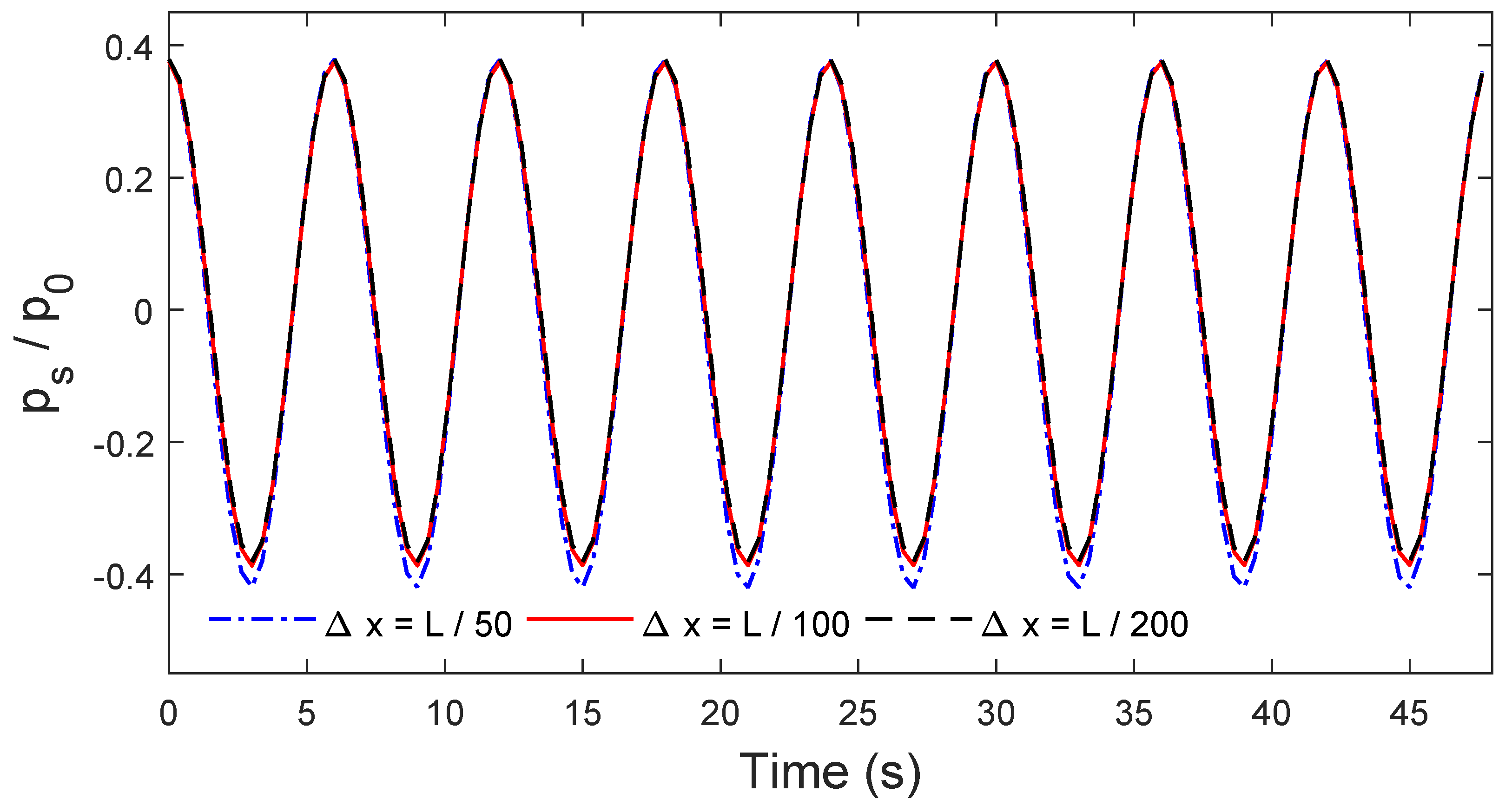
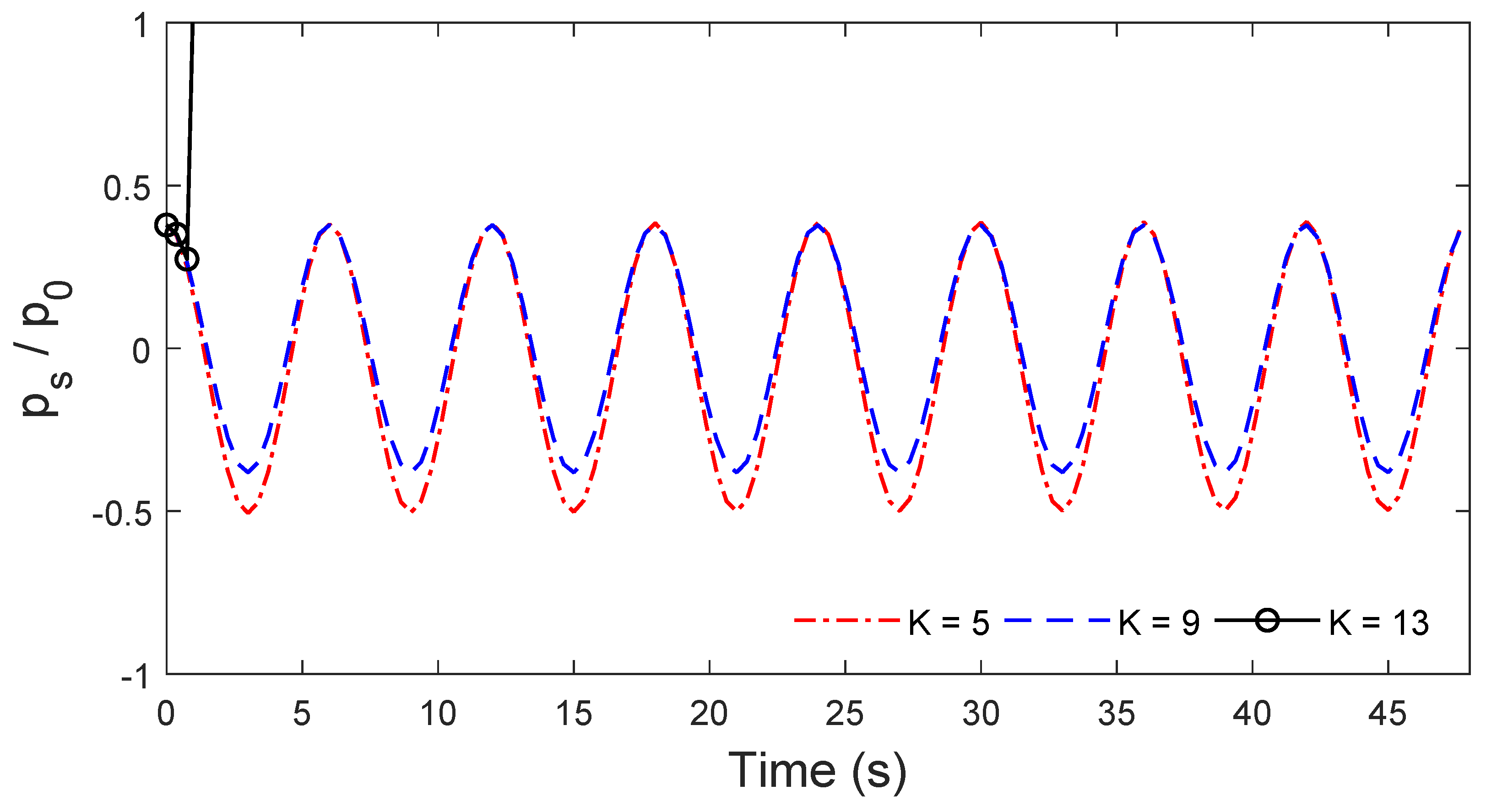
2.6. Convergence Tests

Before conducting parametric studies of the wave-induced dynamic response in a porous seabed under wave loading, it is necessary to check the convergence of a newly proposed numerical model. The convergence tests are carried out in regards of the nodes distance size ( Δ x ), shape factor (c) and the node number of the local region (K), which could have an influence on the numerical accuracy and computational efficiency.
Firstly, the small node distance size makes the results more accurate, however, it will result in enormous computational cost. As shown in Figure 2, the Δ x is equal to L / 50 , L / 100 , and L / 200 respectively (L is the wavelength). The non-dimensional pore water pressures ( p s / p 0 ) are depicted, p 0 represents the amplitude of linear wave pressure at the seabed surface. From the figure, the result for the case of Δ x equal to L / 50 is slightly difference from the others, while the results are almost the same for Δ x equal to L / 100 and L / 200 , which indicate the model is convergent with a node distance that is smaller than L / 100 .
Next, the convergence test of shape factor is conducted.The shape factor is generally equal to 15–60 times the maximum Euclidean distance between two adjacent nodes by convention. The c adopts 3.975 (15 × Δ x ), 7.95 (30 × Δ x ), and 15.9 (60 × Δ x ) separately. From the Figure 3, it can be conclude that the numerical results are not sensitive to the affect the shape factor on the consequence of the almost the same results obtained for this set of shape factors.
Moreover, the effect of the number of nearest neighbour nodes in a local region is examined. The dynamic pore water responses in a seabed are depicted in Figure 4 regards for the different numbers of neighbour nodes in the local region, which are 5, 9 and 13, respectively. From the figure, the result shows a good tendency during the whole process when K = 9 . It also can be seen that for K = 5 , the amplitude of the result is slightly different with the result of K = 9 . When K = 13 , the value of | p s | / p 0 is even beyond 1 after 2 s, which is obviously wrong. This condition might be the ill-condition in this case. Thus, the number of the nodes located in the local region is 9 in this study.

3. Verification of the Proposed Model

Before conducting the parametric study, it is essential to verify the capability of the newly developed meshfree model. In this section, the proposed model is verified by comparison with analytical solutions and a set of published laboratory experiments from a previous study.

3.1. Comparison of the Present Model and the Analytical Solution for Wave-Seabed Interactions

To verify the proposed meshfree model under the dynamic condition, the present model is used to simulate the saturated isotropic seabed under linear wave loading based on a partially dynamic model. The result of the numerical solution are compared with the analytical solution presented by Hsu and Jeng [7]. The linear wave loading is applied to the seabed surface. The parameters for the comparison are given as: wave period T = 10 s; water depth d = 20 m; degree of saturation S r = 0.975 ; Poisson’s ratio ν s = 0.4 ; soil porosity n s = 0.35 ; soil permeability K s = 10 2 m/s; shear modulus G = 5 × 10 6 Pa.
The vertical distributions of the wave-induced pore pressure ( | p s | / p 0 ), effective stresses ( | σ z | / p 0 ) and shear stress ( | τ x z | / p 0 ) versus the soil depth ( z / H ) in a porous seabed are plotted in Figure 5. As depicted in the figure, the blue lines represent the results obtained from analytical solution, while red circles denote soil behaviour simulated from the present “ u p ” time-dependent model. The figure clearly shows that the result obtained by the numerical method are in a good agreement with that of analytical solution, which demonstrates the capability of meshfree model for seabed dynamic response simulation.

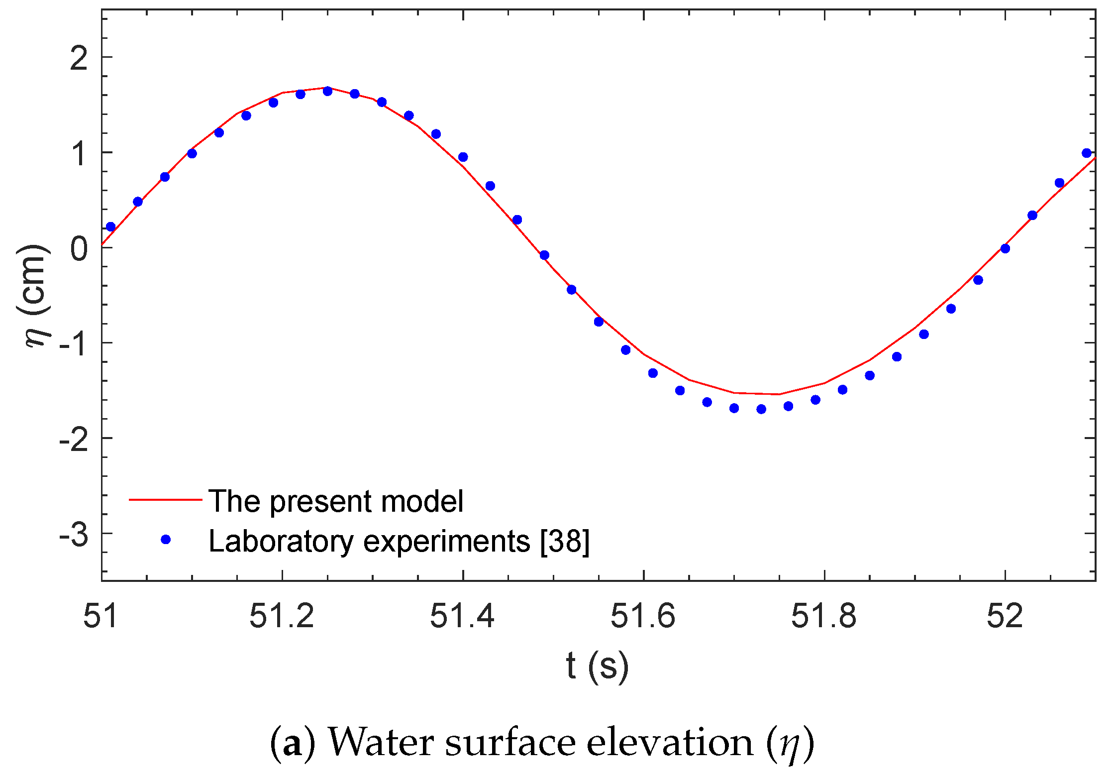
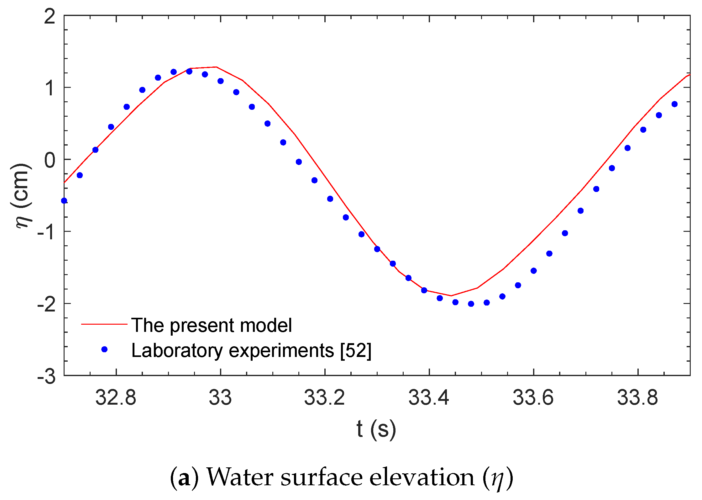
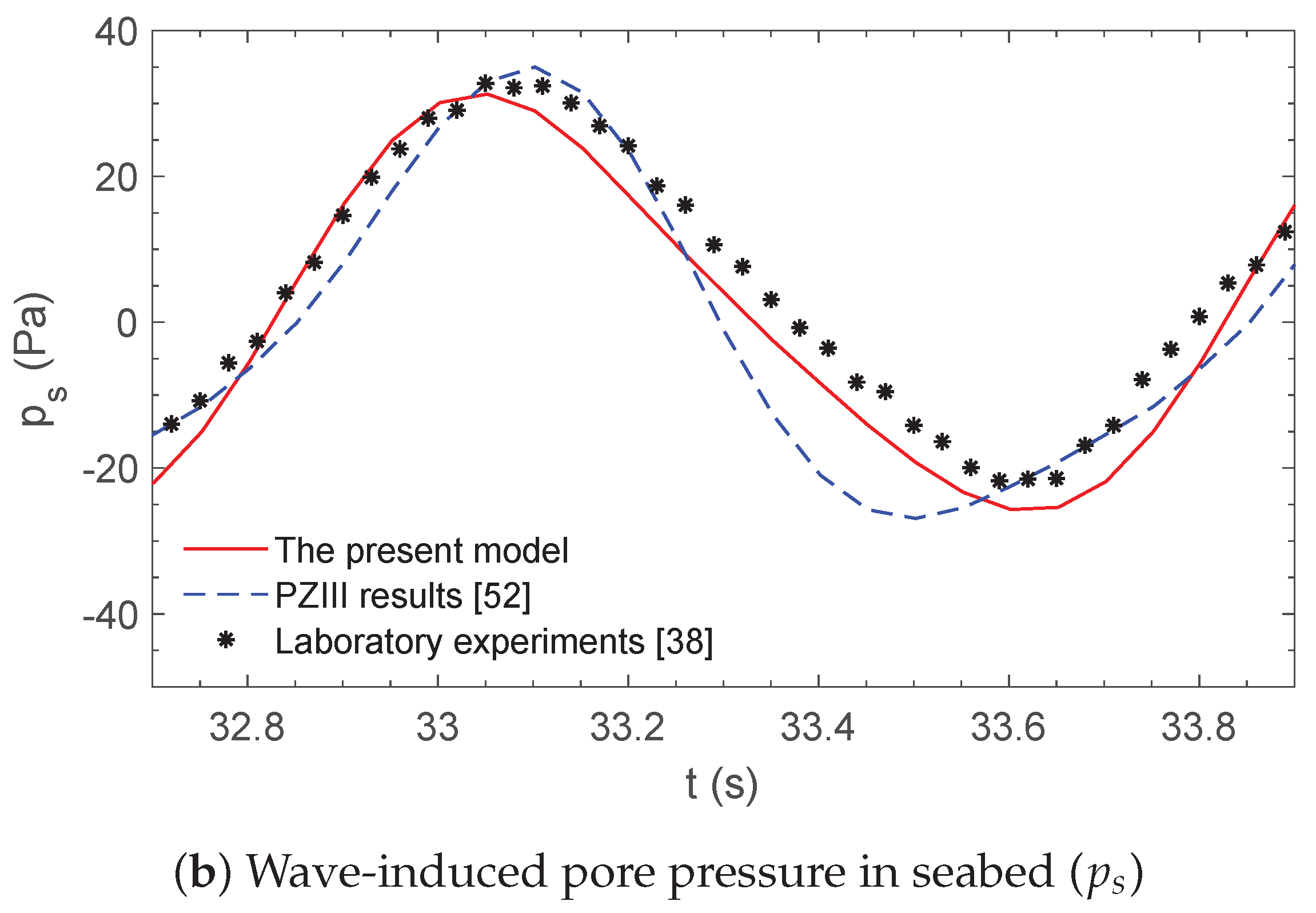
3.2. Comparison of the Present Model with the Laboratory Experiments and Fem Results for Combined Waves and Current Loading

It is necessary to verify the performance of the integration model including both fluid and soil models under the circumstance of complex nature loading. There are numerous laboratory experiments related to the seabed response around the marine structures to date. However, it is quite limited in terms of the experimental data available for the case of immersed tunnel. Thus, the verifications of the integration model are carried out by comparison with the laboratory experiments and the FEM (Finite Element Method) results from DIANA-SWANDYNE II [52] for the seabed without the structure instead in this section. Qi and Gao [38] conducted a series of flume tests considering wave and wave combined currents as dynamic loading, respectively.
The first validation of this section is compared to the laboratory experiments conducted under wave loading only [38]. The input data for the first validation are: wave height H = 0.12 m, water depth d = 0.5 m, wave period T = 1.4 s, seabed thickness h = 1.2 m, degree of saturation S r = 1.0 , shear modulus G = 10 7 N/m 2 , Poisson’s ratio ν s = 0.3 , permeability K s = 1.88 × 10 4 m/s. Figure 6 depicts the wave patterns with corresponding dynamic pore water pressure of the seabed, which are predicted by the present model and obtained from the experiment and FEM model separately. It can be seen that the result obtained from both the wave model and seabed model are in good agreement with the test data, which indicate that the present model is capable for simulating the wave motion in the fluid domain as well as the corresponding soil response of a sandy seabed.
The second validation in this section is to compare with the previous laboratory experiments conducted by Qi and Gao [38]. Unlike the previous case, this test simulates the seabed dynamic response under wave and current, which are generated synchronously. The following current with velocity of 0.05 m/s is adopted. The wave parameters and the soil properties are the same as above. As shown in Figure 7, the fluid pattern tracked by the fluid model matches well with the experiment data, while the pore water pressure simulated by the present model in correspondence with that obtained from the experiment and the FEM model. Thus, the current model performs well for simulating a more realistic marine dynamic elastic behaviour including both the fluid and soil parts.

4. Dynamic Response of the Seabed

In this study, a new meshfree model is developed, based on Biot’s “ u p ” approximation to simulate the dynamic sandy seabed behaviour around an immersed tunnel under complex natural loading including wave and current. As shown in Figure 8, the external loadings are assumed to be propagating over the porous seabed in which the immersed tunnel is buried. The buried depth is defined as b adopting 0.5 m below the seabed surface in this case. The sandy seabed foundation is treated as an elastic two-phase medium above a rigid impermeable bottom with 200 m for seabed length ( L x ) and 40 m for seabed thickness (h). The seawater depth is specified as d. The immersed tunnel is assumed to be placed on the trench dredged on the middle of the seabed of the computational domain. The trench is back-filled by the same type of loose sand with the seabed soil. The tunnel geometry, wave profile and seabed profile in this case are roughly the same as the actual conditions of the Hong Kong–Zhuhai–Macao bridge tunnel, which could provide a reference of the sandy seabed dynamic for such a large immersed tunnel under wave loading.
The detailed dimensions of the immersed tunnel are given in the Figure 9. As shown in figure, the immersed tunnel in this study is considered as an elastic material comprising two traffic tubes of 30 m long and 9 m high (cross section). The boundary condition of the immersed tunnel is treated as impermeable with zero pore pressure gradient. No relative displacement is assumed between the seabed soil and the tunnel frame on the consequence of the high fraction exists between the concrete tunnel surface and seabed soil.
The configuration of the fluid domain and seabed domain can be found in Table 1, as well as the wave characteristics, seabed soil properties and modelling parameters. The seabed foundation is assumed to be composed of relative dense deposited sand [53]. Figure 10 shows the applicability range of the different wave theories [54]. The wave characteristics adopted in this study are in the range of Stokes second-order wave ( H = 4 m, T = 10 s, d = 30 m, shown as a red star in Figure 10), which is generated and simulated by fluid model. The node number of the local region (K) for local RBF method is 9, while a positive constant c which is known as the shape factor equals 6. The total number of nodes in this case is 771,140. The convergence test has been done to check the stability of the present parameter configuration, which is quite enough to obtain an accuracy and detailed result. The time step Δ t set in this case is 0.5 s, while 20 time steps are contained in one wave period.
The aim of this section is tracking the dynamic soil response during the wave propagating over the seabed around the immersed tunnel. During the wave propagation from the left to the right of the computational domain continuously, the effective stresses and pore water pressures show a correlation trend with the change of the water pressure acting on the surface of the seabed. As shown in Figure 11, the oscillatory wave-induced pore water pressures, horizontal displacements ( u s ) and vertical displacement ( w s ) for the computational domain of the seabed at t = 13 s are presented, respectively. It is found that the seabed dynamic behaviour with immersed tunnel is not periodic symmetry any more under the cyclic wave loading. The figure shows that the existence of the immersed tunnel has an obvious influence on the dynamic behaviour of the sandy seabed soil nearby by comparing the region located on the leftward and the rightward of the tunnel. It can be seen in Figure 11 that the placement of a tunnel weakens the displacement change of local area in a way, while the fluctuation of the dynamic pore water pressure decrease around as well. In Figure 11c, the dynamic pore water pressure of the seabed soil beneath the tunnel bottom shows a different tendency from the surrounding that the positive oscillatory pore pressure occurs on the left corner while the negative occurs on the right corner. In order to figure out a more detailed dynamic soil response in the vicinity of the immersed tunnel, the results of dynamic pore water pressure of some typical locations are analysed.
As shown in Figure 8, points A to D are a set of symmetrical nodes about the tunnel at the depth of −5 m in the seabed ( x = 60, 82, 118, 140 m, respectively), while points E to F located at the depth of −10 m ( x = 60, 85, 115, 140 m respectively). Points F and G are set on 0.5 m below the two base corners of the immersed tunnel. Figure 12 depicts the time series of the dynamic pore water pressure generated by the two point sets. From the figure, it can be seen that the vibration of the pore water pressure is more violent on the remote seabed from the tunnel, which is consistent with the conclusion mentioned above. Furthermore, the amplitude reduced for point F and G below the tunnel are slightly less than the points B and C on two sides of the tunnel. The pore water pressure vibration of the soil on points F and G is even larger than on points B and C, which indicates that the seabed foundation beneath the immersed tunnel is more likely to be unstable due to transient liquefaction. In addition, a phenomenon occurred which is that there is a phase difference of dynamic pore pressure brought out under the base corners of the tunnel (points F and G), as shown in Figure 12b.

5. Wave-Induced Liquefaction

The stability of the coastal structures and its seabed foundation is one of the main concerns for engineering design procedure. The wave-induced liquefaction in a porous seabed is one of the most significant unstable factors. Zen and Yamazaki [55] pointed out that the liquefaction of the porous seabed is responding to the variation of the ocean wave, which is actually caused by the periodic upward seepage force. Thus, we proposed to estimate the liquefaction state in two-dimensions, i.e.,
σ 0 + ( P b p s ) 0
where σ 0 represents the initial effective stress, P b is the wave pressure acting on seabed, while p s is the wave-induced transient pore pressure. The value of P b p s is equal to the excess pore pressure generated by the wave loading ( | u e | ).
Figure 13 shows the wave-induced transient liquefaction area around the immersed tunnel at three typical times ( t = 12 s, t = 14 s and t = 15.5 s) separately. As shown in the figure, the transient liquefaction area moves along the direction of the wave propagation. The previously liquefied area is able to recover as the wave trough go away. This process is repeated periodically under the cyclic wave loading. The maximum liquefaction depth in this case is 0.8 m below the seabed surface, as seen in Figure 13a, while the soil that covered the tunnel is fully liquefied during one wave period which illustrated in Figure 13b. Thus, the back filling soil above the tunnel can not protect the immersed tunnel any more in this circumstance. Moreover, the maximum liquefaction depth of the rightward seabed of the tunnel is 0.6 m, which is slightly shallow than that in leftwards of 0.8 m.

6. Parametric Study

In this section, parametric studies of the seabed liquefaction around the immersed tunnel are carried out, which include the wave characteristics, soil properties and the effects of current specifically.

6.1. Effects of Wave Characteristics

Basically, the wave-induced oscillatory liquefaction phenomenon of the porous seabed is highly relative to the water pressure propagating on it. As a consequence, the relation of the wave characteristics and the liquefaction depth in the vicinity of the tunnel is discussed in detail with respect to the wave period (T), wave height (H), and still water depth (d), separately. Table 2 lists the input data involving the wave variables and other parameters. Figure 14 characterizes the maximum liquefaction depth of the vertical section at x = 80 m which is on the left side of the tunnel in regard of the different wave conditions.
It is well known that the wave height is in positive correlation to the value of the water pressure acting on the seabed precisely. Furthermore, the water pressure will affect the wave-induced pore water pressure in seabed deposits. As illustrated in Figure 14a, the maximum liquefaction depth grows deeper with an increase of the wave height, which shows the positive relationship between the wave height and the potential of liquefaction.
The wave period is another key wave parameter that influences the wave length directly, which will further affect the seabed transient liquefy process. In this study, the wave periods are from 8 to 10 s. From Figure 14b, the maximum liquefaction depth is progressively increase with the rise of wave periods. It can be concluded that the liquefaction degree is more intense in the case of a long wave period.
Lastly, the influence of still water depth is discussed. The water depth ranges from 30 to 40 m. Unlike wave height and period, the maximum oscillatory liquefaction depth decreases with the raising of still water depth, as shown in Figure 14c, which indicates that the wave-induced transient liquefaction is more likely to occur in the shallow water areas.

6.2. Effects of Soil Properties

Besides the wave characteristics, the deposit conditions are found to be essential in a wave-seabed structure interactions. The effects of two parameters of soil properties are discussed individually, i.e., degree of saturation ( S r ), and soil permeability ( K s ). A series of topical values are selected in this section, which are from 1.0 × 10 5 to 1.0 × 10 3 for soil permeability, and 0.925–0.975 for degree of saturation, respectively. The wave condition and other parameters used in this section can be found in Table 3.
To examine how the different soil parameters affect the seabed liquefaction around the immersed tunnel, Figure 15 and Figure 16 are depicted to show the vertical distribution of the excess pore pressure ( | u e | / σ 0 ) and the maximum liquefaction depth of the vertical section at x = 80 m in seabed with various soil properties. Figure 15b illustrates that the maximum liquefaction depth is larger in the seabed with relative low degree of saturation. While the same conclusion can be draw for the various of soil permeability in Figure 16b, i.e., the smaller the soil permeability adopted, the deeper the liquefaction occurs in the vicinity of the tunnel.

6.3. Effects of Current

In reality, the fluid circumstance above the seabed are quite complex, and need to considered in the wave–current interaction. The motion of the current is able to influence the wave propagation, which further affects the seabed liquefaction process. This section aims to investigate the relationship between seabed liquefaction and the current around the immersed tunnel. The seabed response under a second-order Stokes wave ( T = 10 s, H = 4 m and d = 35 m) with a series of following currents ( U 0 = 0.5, 1.0, 1.5 m/s) and opposing currents ( U 0 = −0.5, −1.0, −1.5 m/s) are compared with the no current case. Other parameters used in this study are listed in Table 4.
As seen in Figure 17, the maximum liquefied depth in seabed around the tunnel ( x = 80 m) is 0.4 m, 0.6 m and 0.7 m when the current velocity U 0 takes on −1.5 m/s, 0 m/s and 1.5 m/s, which indicate the following current could deeper the liquefaction zone while the opposing current could decrease the liquefaction depth. Moreover, Figure 18 shows the liquefaction area around the immersed tunnel (when wave trough travels above the cross section x = 80 m) triggered by the wave combined different currents velocities. It can be concluded that not only the liquefied depth, but the liquefaction zone changes around the tunnel are also positively relative to the velocity of the current. Thus, oscillatory liquefaction is more likely to occur under the following current and the opposing current is able to decrease the potential of liquefaction.

7. Conclusions

In this study, an integrated numerical model including a LRBFCM seabed model based on Biot “ u p ” approximation is proposed to investigate the flow field dynamics and corresponding seabed behaviour around an immersed tunnel under second-order stokes wave combined current with various velocities. The oscillatory liquefaction under the different wave characteristics, soil properties, and current velocities are discussed in detail. From the numerical result, the following conclusions can be drawn:
(1)
The newly developed meshfree model is well validated by comparison with the analytical solution, the laboratory experiments and previous numerical results. The LRBFCM is examined to be reliable in simulation of wave-induced oscillatory liquefaction behaviour of a seabed. Moreover, on the consequence of mesh-independence, the present model is more efficient than the conventional model based on FEM (Finite element method) or FVM (Finite volume method).
(2)
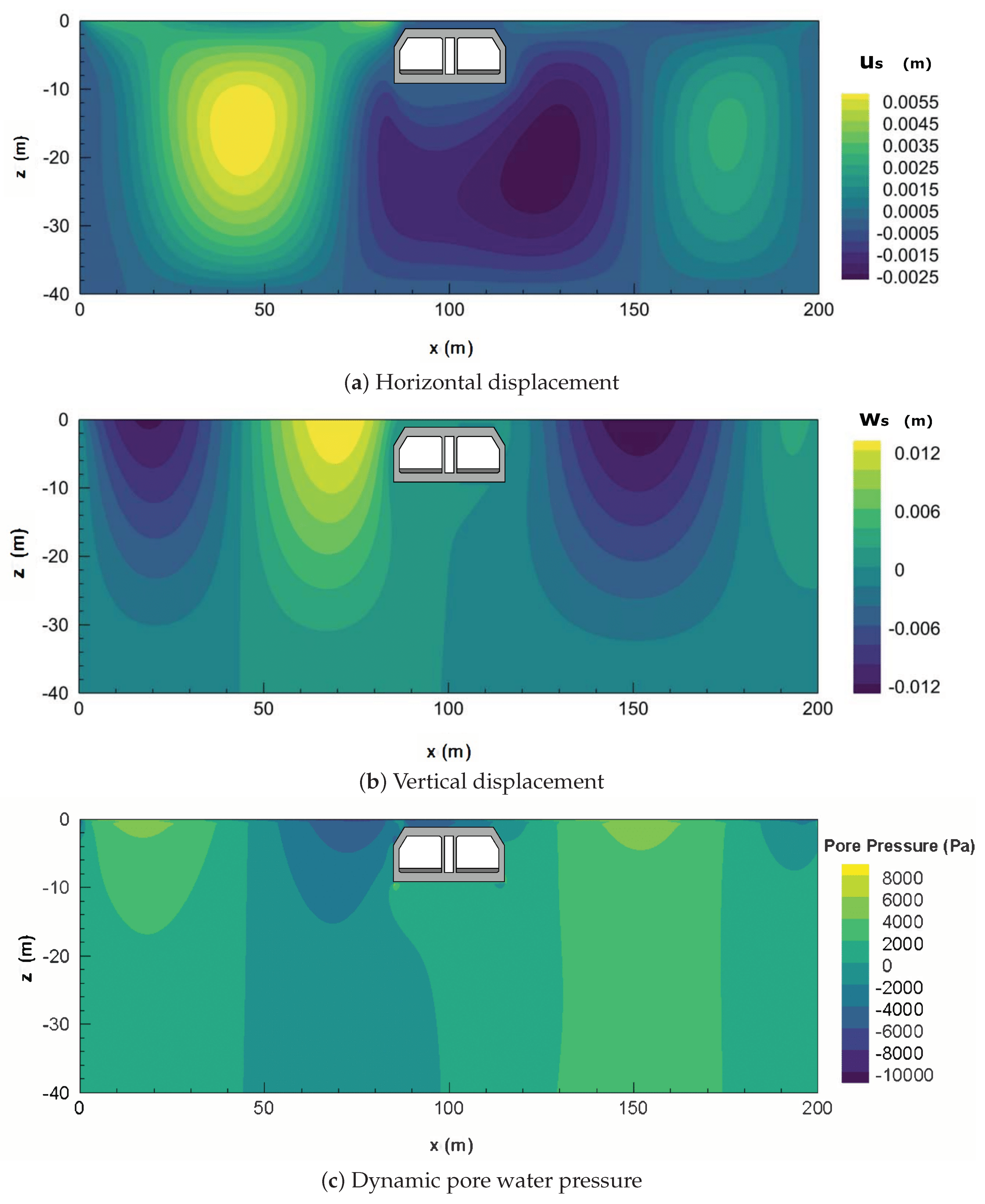
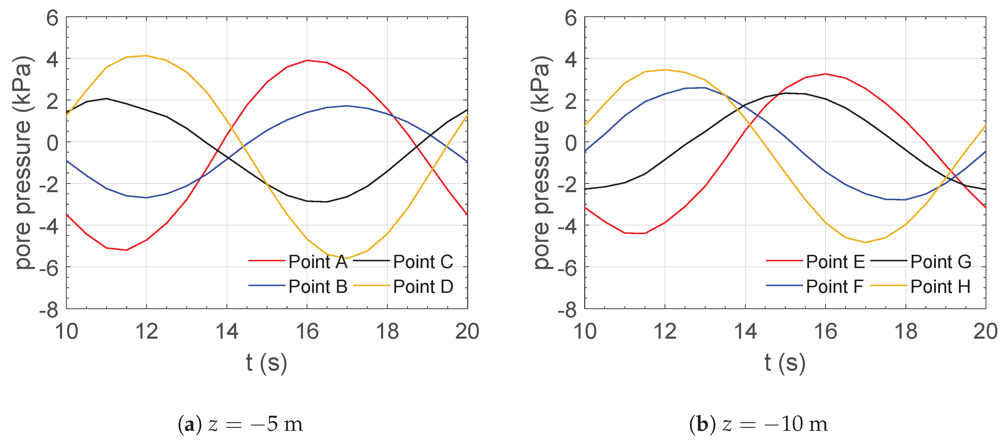
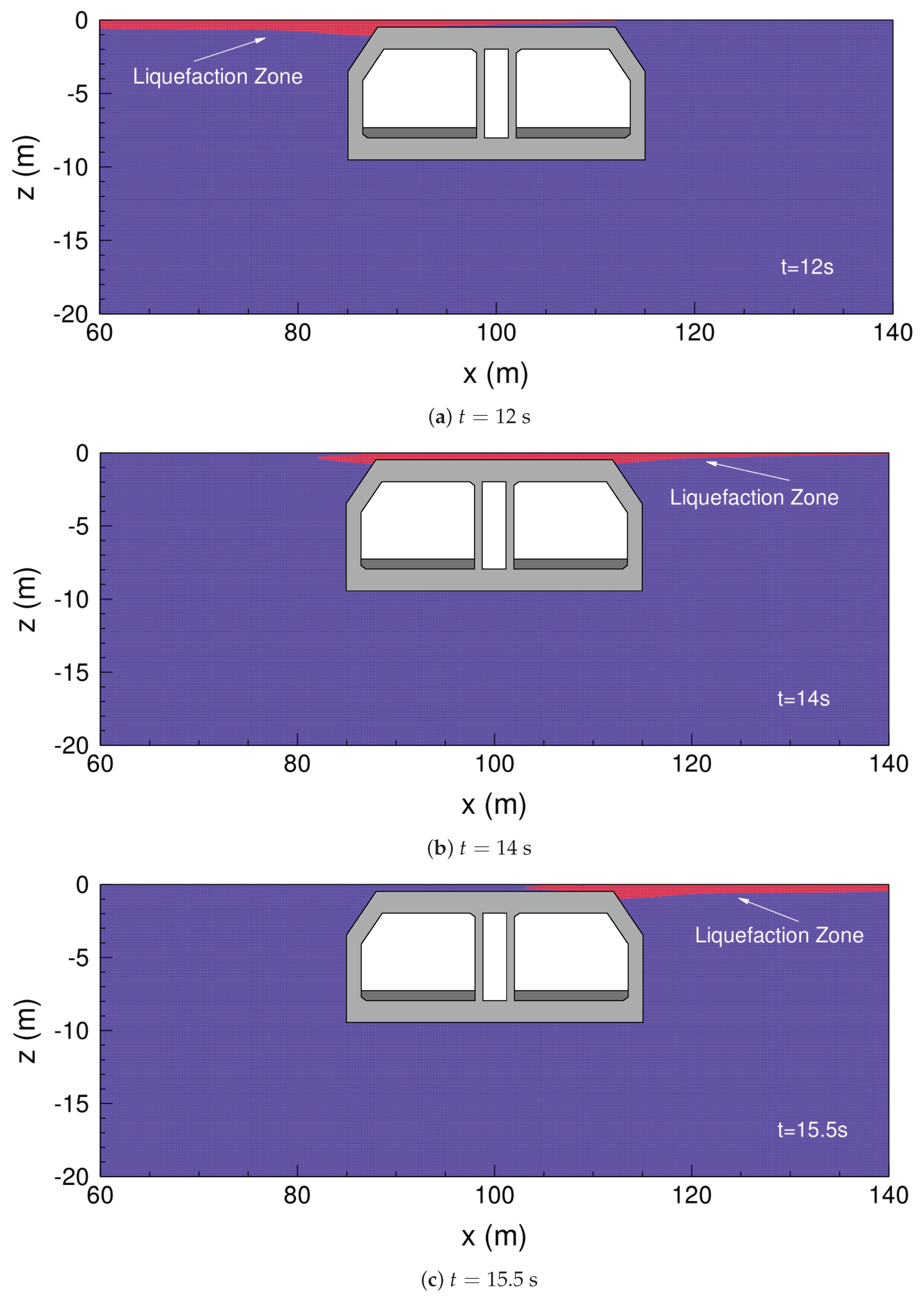
The existence of the immersed tunnel affects surrounding seabed dynamic behaviours, which are able to weaken the displacement and dynamic pore pressure change nearby. Furthermore, the maximum liquefied depth on the right of the tunnel is smaller than that on the left.
(3)
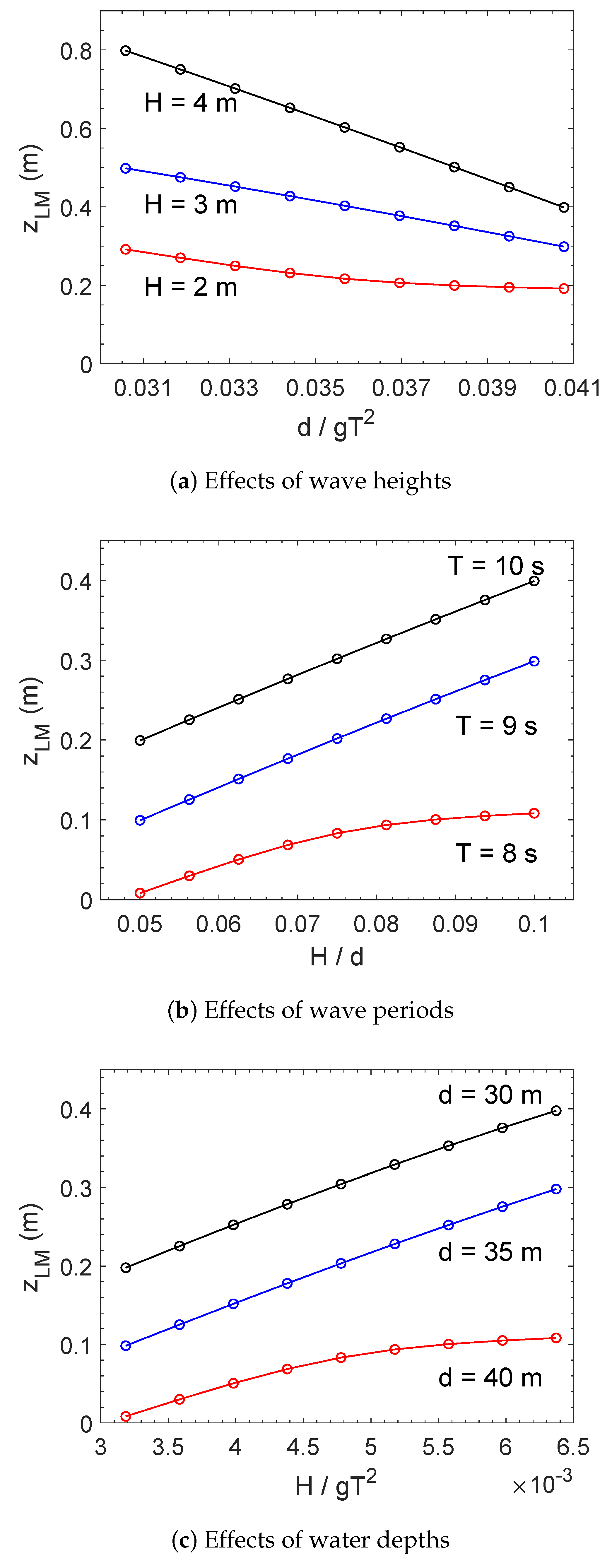
The wave-induced transient liquefaction around the tunnel is highly relative to the wave characteristics. It is found that the seabed liquefaction is more likely to occur under a shallow water area with the waves of large wave height and long period.
(4)
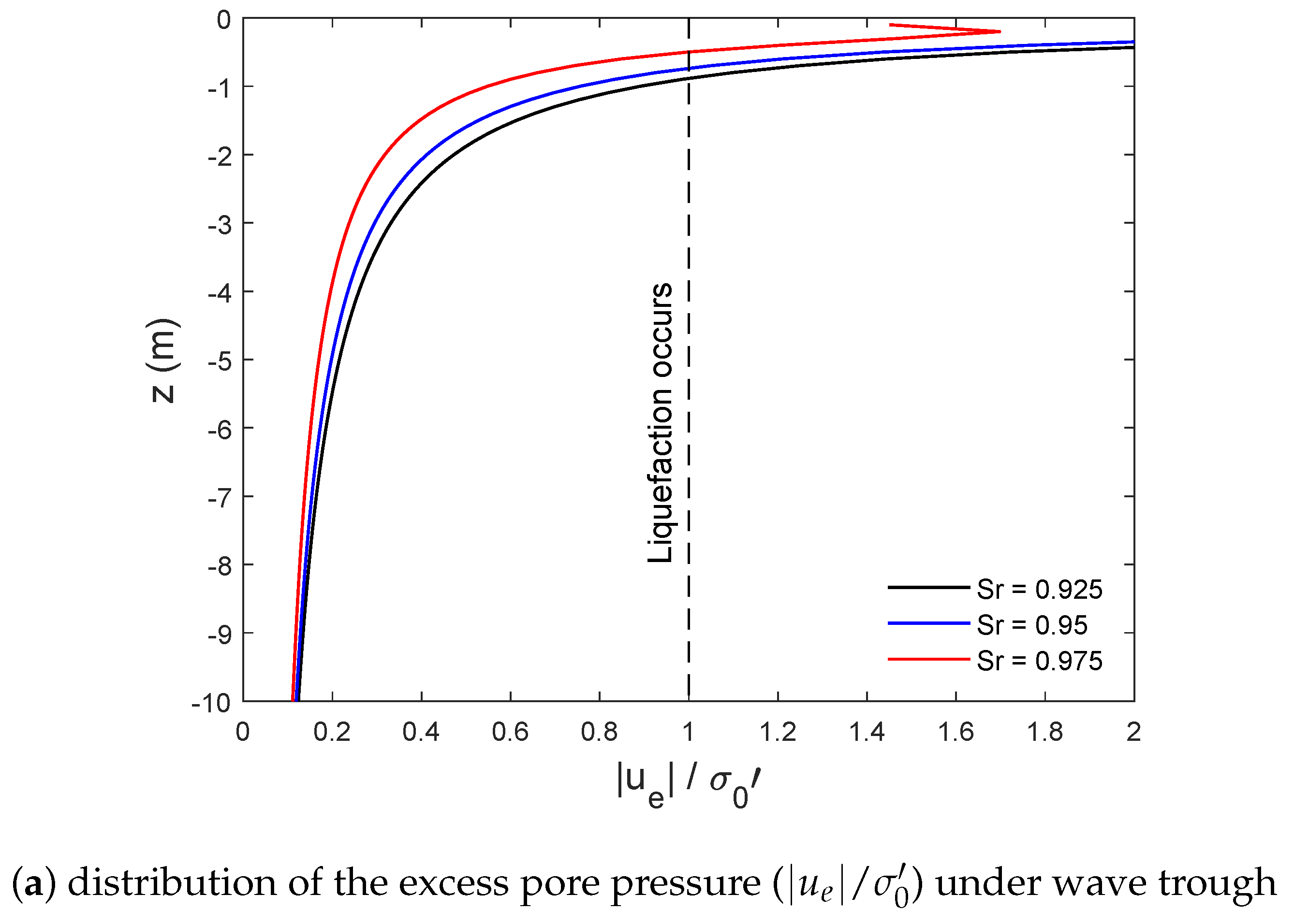
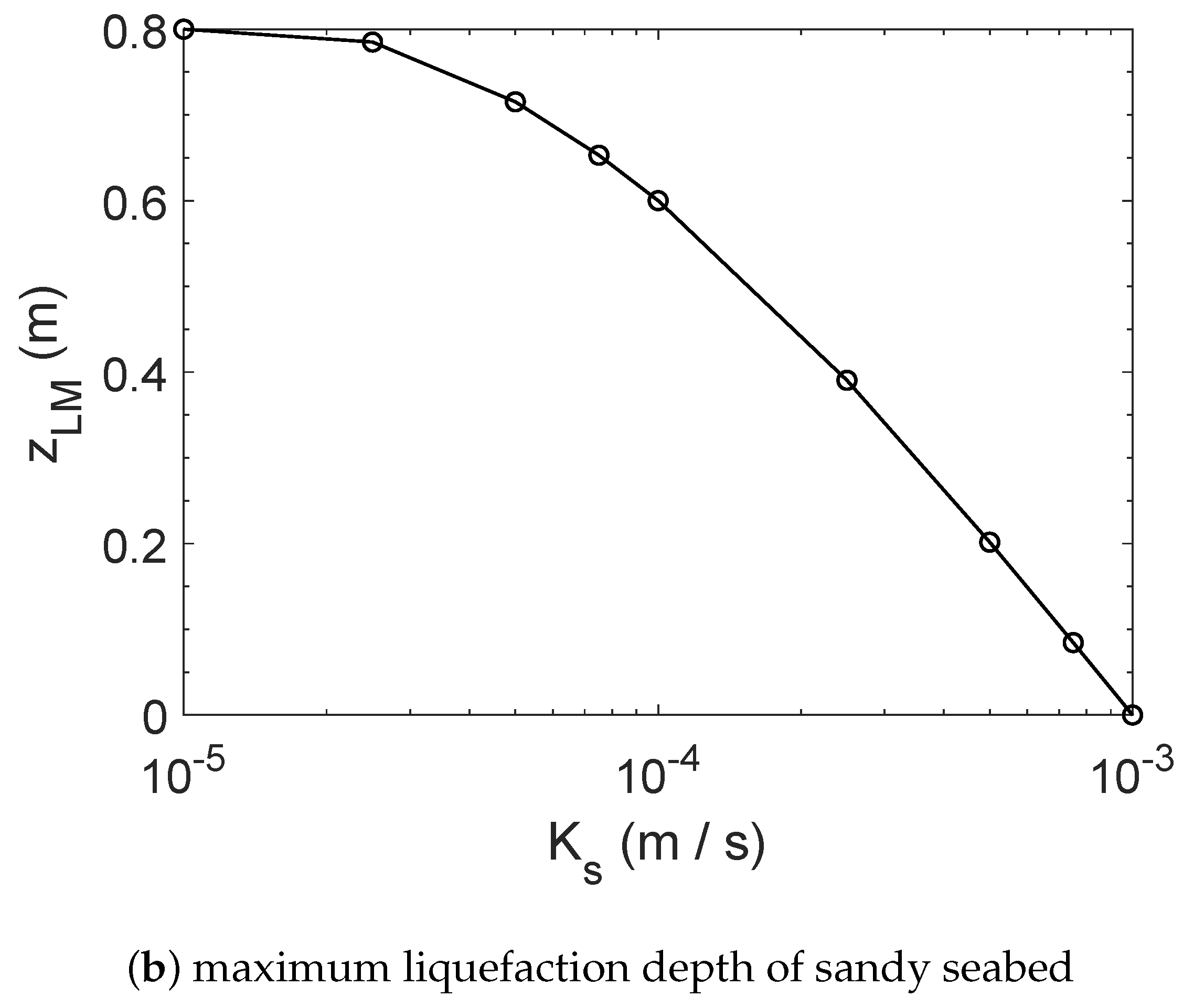
The parametric studies show that the soil properties around tunnel have a significant impact on the liquefaction behaviour as well. The smaller the soil permeability and degree of saturation adopted, the deeper the liquefaction occurs in the vicinity of the tunnel.
(5)
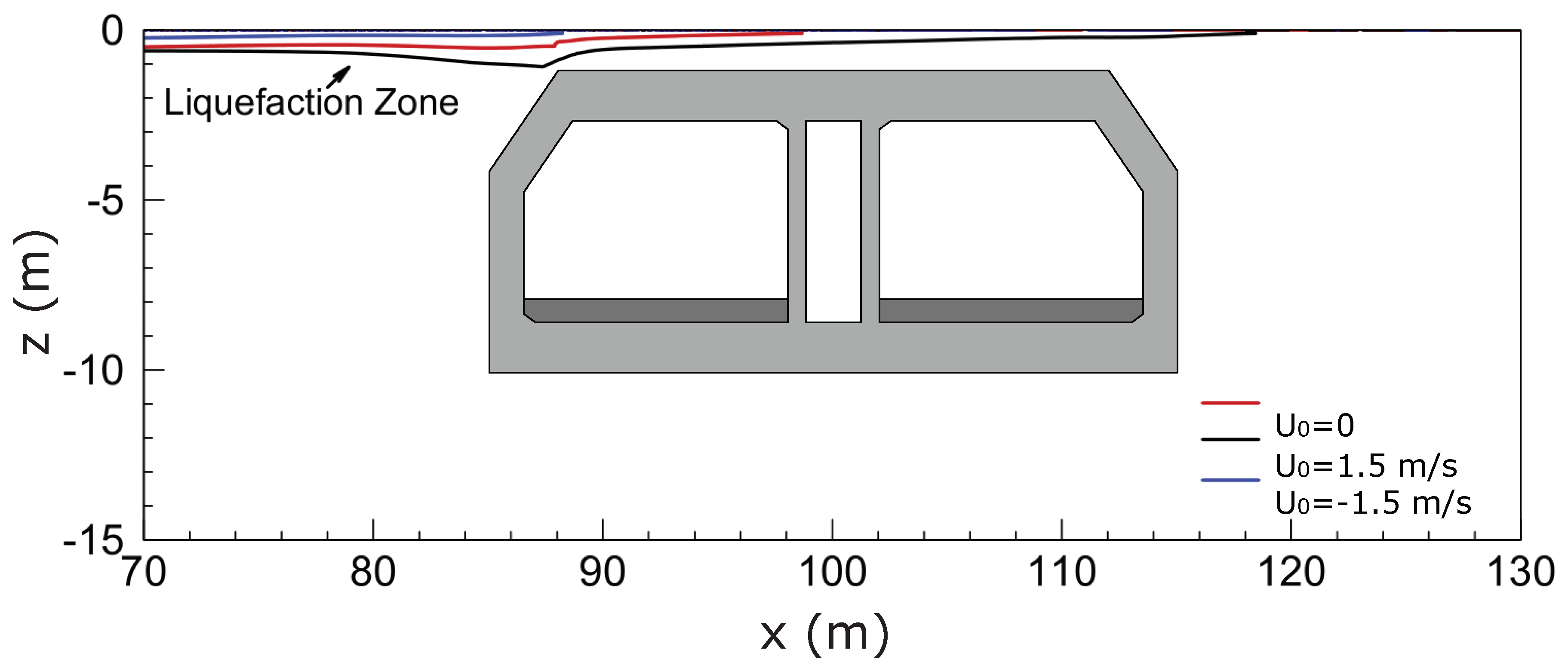
Based on the numerical result, the occurrence of currents could obviously affect wave-induced liquefaction. The following current can aggravate the seabed liquefaction while the opposing current can decrease the liquefied risk around the tunnel.

Author Contributions

Conceptualization, D.-S.J.; methodology, C.-C.T. and S.H.; validation, S.H.; formal analysis, S.H.; writing—original draft preparation, S.H.; writing—review and editing, D.-S.J. and C.-C.T.; supervision, D.-S.J. and C.-C.T.

Funding

This research received funding from the Ministry of Science and Technology of Taiwan under the grant no. MOST 106-2918-I-022-001.

Acknowledgments

The first author is grateful for the support of High Performance Computing Cluster “Gowanda” to complete this research, and the supporting of scholarship from Griffith University. The third author is grateful for the support of the Ministry of Science and Technology of Taiwan under the grant no. MOST 106-2918-I-022-001.

Conflicts of Interest

The authors declare no conflict of interest.

Abbreviations

p 0 The amplitude of linear wave pressure at the seabed surface
P b The dynamic wave pressure at the seabed surface
γ ω Unit weight of water
n s Soil porosity
β s The compressibility of pore fluid
K f The bulk modulus of pore fluid
Darcy’s volume-averaging operator
f The intrinsic averaging operator
ρ w a t e r , ρ a i r Density of water and air
ρ f , ρ s Density of fluid and solid
ρ Average density of a porous seabed
α The indicator function
u i The velocity vector
g i The gravitational acceleration
μ e f f The efficient dynamic viscosity
μ The molecular dynamic viscosity
ν t u r b The turbulent kinetic viscosity
d 50 The medium grain diameter of the material
K C The Keulegan-Carpenter number
T 0 The period of the oscillatory
Φ w a t e r , Φ a i r Water and air properties
σ x , σ z The effective normal stresses in the x- and z-directions
σ 0 The initial effective stress
τ x z The shear stress
u s , w s The soil displacement in the x- and z-directions
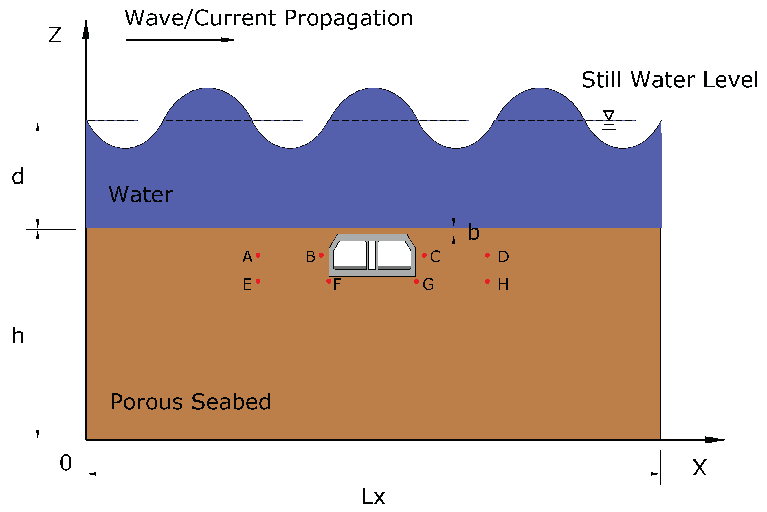
bTunnel buried depth
K w The true bulk modulus of the elasticity of water
S r The degree of saturation
P w o The absolute water pressure
p s The pore water pressure
u e The excess pore pressure geberated by the wave loading
α m The undetermined coefficient related to RBF of a linear equation
p The psedo-dynamic pressure
GThe shear modulus
KThe number of nearest neighbour nodes
HWave height
dWater depth
hSeabed thickness
TWave period
U 0 Current velocity
ν s Poisson’s ratio
K s Soil permeability
η Wave profile
EYoung’s modulus
LWavelength
L x Seabed length
zSoil depth
κ The turbulence kinetic energy
ϵ The turbulence energy dissipation rate
ϵ s The volume strain
C μ An empirical constant relate to the turbulent viscosity
cShape factor
N d t Time steps in a period
FEMFinite Element Method
FVMFinite Volume Method
VARANSVolume-Average Reynolds-Average Navier-Stokes
VOFVolume of fluid
2DTwo-dimensional
3DThree-dimensional
LRBFCMLocal radial basis function collocation method
MLSMoving least-square method
PIMPoint interpolation method
RBFRadial basis function
MQMultiquadrics
GRBFCMGlobal radial basis function collocation method

References

  1. Zen, K.; Yamazaki, H. Mechanism of wave-induced liquefaction and densification in seabed. Soils Found. 1990, 30, 90–104. [Google Scholar] [CrossRef]
  2. Sumer, B.M.; Fredsøe, J. The Mechanics of Scour in the Marine Environment; World Scientific Publishing Co. Pte. Ltd.: Singapore, 2002. [Google Scholar]
  3. Jeng, D.S. Mechanics of Wave-Seabed-Structure Interactions: Modelling, Processes and Applications; Cambridge University Press: Cambridge, MA, USA, 2018. [Google Scholar]
  4. Yamamoto, T.; Koning, H.; Sellmeijer, H.; Hijum, E.V. On the response of a poro-elastic bed to water waves. J. Fluid Mech. 1978, 87, 193–206. [Google Scholar] [CrossRef]
  5. Seed, H.B.; Rahman, M.S. Wave-induced pore pressure in relation to ocean floor stability of cohesionless soils. Mar. Geotechnol. 1978, 3, 123–150. [Google Scholar] [CrossRef]
  6. Jeng, D.S.; Seymour, B.R. A simplified analytical approximation for pore-water pressure build-up in a porous seabed. J. Waterw. Port Coast. Ocean Eng. ASCE 2007, 133, 309–312. [Google Scholar] [CrossRef]
  7. Hsu, J.R.C.; Jeng, D.S. Wave-induced soil response in an unsaturated anisotropic seabed of finite thickness. Int. J. Numer. Anal. Methods Geomech. 1994, 18, 785–807. [Google Scholar] [CrossRef]
  8. Jeng, D.S. Porous Models for Wave-Seabed Interactions; Springer Science & Business Media: Berlin/Heidelberg, Germany, 2013. [Google Scholar]
  9. Jeng, D.S.; Ye, J.H.; Zhang, J.S.; Liu, P.L.F. An integrated model for the wave-induced seabed response around marine structures: Model verifications and applications. Coast. Eng. 2013, 72, 1–19. [Google Scholar] [CrossRef]
  10. Zhao, H.Y.; Jeng, D.S. Accumulation of pore pressures around a submarine pipeline buried in a trench layer with partially backfills. J. Eng. Mech. ASCE 2016, 142, 04016042. [Google Scholar] [CrossRef]
  11. Kasper, T.; Steenfelt, J.; Pedersen, L.; Jackson, P.; Heijmans, R. Stability of an immersed tunnel in offshore conditions under deep water wave impact. Coast. Eng. 2008, 55, 753–760. [Google Scholar] [CrossRef]
  12. Chen, W.; Fang, D.; Chen, G.; Jeng, D.; Zhu, J.; Zhao, H. A simplified quasi-static analysis of wave-induced residual liquefaction of seabed around an immersed tunnel. Ocean Eng. 2018, 148, 574–587. [Google Scholar] [CrossRef]
  13. Chen, W.Y.; Liu, C.L.; Duan, L.L.; Qiu, H.M.; Wang, Z.H. 2D Numerical study of the stability of trench under wave action in the immersing process of tunnel element. J. Mar. Sci. Eng. 2019, 7, 57. [Google Scholar] [CrossRef]
  14. CCCC Second Flight Engineering Survey & Design Institute Co., Ltd. (CCCC SFES & DI). Geological Investigation Report on Immersed Tunnel of Hong Kong-Zhuhai-Macao Bridge in Construction Documents Design Phase; CCCC Second Flight Engineering Survey & Design Institute Co., Ltd.: Guangzhou, China, 2009. (In Chinese) [Google Scholar]
  15. Ye, J.; Jeng, D.S. Response of seabed to natural loading-waves and currents. J. Eng. Mech. ASCE 2012, 138, 601–613. [Google Scholar] [CrossRef]
  16. Wen, F.; Jeng, D.S.; Wang, J.H. Numerical modeling of response of a saturated porous seabed around an offshore pipeline considering non-linear wave and current interactions. Appl. Ocean Res. 2012, 35, 25–37. [Google Scholar] [CrossRef]
  17. Liao, C.C.; Jeng, D.-S.; Lin, Z.; Guo, Y.; Zhang, Q. Wave (current)-induced pore pressure in offshore deposits: A coupled finite element model. J. Mar. Sci. Eng. 2019, 6, 83. [Google Scholar] [CrossRef]
  18. Nayroles, B.; Touzot, G.; Villon, P. Generalizing the finite element method: Diffuse approximation and diffuse elements. Comput. Mech. 1992, 10, 307–318. [Google Scholar] [CrossRef]
  19. Belytschko, T.; Lu, Y.Y.; Gu, L. Element-free Galerkin methods. Int. J. Numer. Methods Eng. 1994, 37, 229–256. [Google Scholar] [CrossRef]
  20. Liu, G.R.; Gu, Y. A point interpolation method for two-dimensional solids. Int. J. Numer. Methods Eng. 2001, 50, 937–951. [Google Scholar] [CrossRef]
  21. Wang, J.; Liu, G.; Lin, P. Numerical analysis of biot’s consolidation process by radial point interpolation method. Int. J. Solids Struct. 2002, 39, 1557–1573. [Google Scholar] [CrossRef]
  22. Wang, J.; Liu, G. On the optimal shape parameters of radial basis functions used for 2-D meshless methods. Comput. Methods Appl. Mech. Eng. 2002, 191, 2611–2630. [Google Scholar] [CrossRef]
  23. Hardy, R.L. Theory and applications of the multiquadric-biharmonic method 20 years of discovery 1968–1988. Comput. Math. Appl. 1990, 19, 163–208. [Google Scholar] [CrossRef]
  24. Powell, M. The theory of radial basis function approximation in 1990, Advances in Numerical Analysis II: Wavelets, Subdivision, and Radial Functions (WA Light, ed.). Oxf. Univ. Press. Oxf. 1992, 105, 210. [Google Scholar]
  25. Kansa, E.J. Multiquadrics—A scattered data approximation scheme with applications to computational fluid-dynamics—II solutions to parabolic, hyperbolic and elliptic partial differential equations. Comput. Math. Appl. 1990, 19, 147–161. [Google Scholar] [CrossRef]
  26. Mai-Duy, N.; Tran-Cong, T. Indirect RBFN method with thin plate splines for numerical solution of differential equations. CMES Comput. Model. Eng. Sci. 2003, 4, 85–102. [Google Scholar]
  27. Šarler, B.; Perko, J.; Chen, C.S. Radial basis function collocation method solution of natural convection in porous media. Int. J. Numer. Methods Heat Fluid Flow 2004, 14, 187–212. [Google Scholar] [CrossRef] [Green Version]
  28. Wu, N.J.; Chang, K.A. Simulation of free-surface waves in liquid sloshing using a domain-type meshless method. Int. J. Numer. Methods Fluids 2011, 67, 269–288. [Google Scholar] [CrossRef]
  29. Kovacevic, I.; Poredos, A.; Sarler, B. Solving the Stefan problem with the radial basis function collocation method. Numer. Heat Transf. Part B Fundam. 2003, 44, 575–598. [Google Scholar] [CrossRef]
  30. Hardy, R.L. Multiquadric equations of topography and other irregular surfaces. J. Geophys. Res. 1971, 76, 1905–1915. [Google Scholar] [CrossRef]
  31. Lee, C.K.; Liu, X.; Fan, S.C. Local multiquadric approximation for solving boundary value problems. Comput. Mech. 2003, 30, 396–409. [Google Scholar] [CrossRef]
  32. Šarler, B.; Vertnik, R. Meshfree explicit local radial basis function collocation method for diffusion problems. Comput. Math. Appl. 2006, 51, 1269–1282. [Google Scholar] [CrossRef] [Green Version]
  33. Kosec, G.; Sarler, B. Local RBF collocation method for Darcy flow. Comput. Model. Eng. Sci. 2008, 25, 197–208. [Google Scholar]
  34. Tsai, C.C.; Lin, Z.H.; Hsu, T.W. Using a local radial basis function collocation method to approximate radiation boundary conditions. Ocean Eng. 2015, 105, 231–241. [Google Scholar] [CrossRef]
  35. Kosec, G.; Založnik, M.; Šarler, B.; Combeau, H. A meshless approach towards solution of macrosegregation phenomena. Comput. Mater. Contin. 2011, 22, 169–195. [Google Scholar]
  36. Wang, X.X.; Jeng, D.S.; Tsai, C.C. Meshfree model for wave-seabed interactions around offshore pipelines. J. Mar. Sci. Eng. 2019, 7, 87. [Google Scholar] [CrossRef]
  37. Higuera, P.; Lara, J.L.; Losada, I.J. Realistic wave generation and active wave absorption for Navier-Stokes models: Application to OpenFOAM. Coast. Eng. 2013, 71, 102–118. [Google Scholar] [CrossRef]
  38. Qi, W.G.; Gao, F.P. Physical modelling of local scour development around a large-diameter monopile in combined waves and current. Coast. Eng. 2014, 83, 72–81. [Google Scholar] [CrossRef]
  39. Ahmad, N.; Bihs, H.; Chella, M.A.; Arntsen, Ø.A.; Aggarwal, A. Numerical modelling of arctic coastal erosion due to breaking waves impact using REEF3D. In Proceedings of the 27th International Ocean and Polar Engineering Conference, International Society of Offshore and Polar Engineers, San Francisco, CA, USA, 25–30 June 2017. [Google Scholar]
  40. Nangia, N.; Patankar, N.A.; Bhalla, A.P.S. A DLM immersed boundary method based wave-structure interaction solver for high density ratio multiphase flows. arXiv 2019, arXiv:1901.07892. [Google Scholar] [CrossRef]
  41. De Jesus, M.; Lara, J.L.; Losada, I.J. Three-dimensional interaction of waves and porous coastal structures: Part I: Numerical model formulation. Coast. Eng. 2012, 64, 57–72. [Google Scholar] [CrossRef]
  42. Engelund, F. On the Laminar and Turbulent Flows of Ground Water through Homogeneous Sand; Akademiet for de Tekniske Videnskaber: København, Denmark, 1953. [Google Scholar]
  43. Burcharth, H.F.; Andersen, O.K. On the one-dimensional steady and unsteady porous flow equations. Coast. Eng. 1995, 24, 233–257. [Google Scholar] [CrossRef]
  44. Higuera, P. Application of Computational Fluid Dynamics to Wave Action on Structures. Ph.D. Thesis, Universidade de Cantabria, Cantabria, Spain, 2015. [Google Scholar]
  45. Zienkiewicz, O.C.; Chang, C.T.; Bettess, P. Drained, undrained, consolidating and dynamic behaviour assumptions in soils. Géotechnique 1980, 30, 385–395. [Google Scholar] [CrossRef]
  46. Biot, M.A. General theory of three-dimensional consolidation. J. Appl. Phys. 1941, 26, 155–164. [Google Scholar] [CrossRef]
  47. Bentley, J.L. Multidimensional binary search trees used for associative searchings. Commun. ACM 1975, 18, 509–517. [Google Scholar] [CrossRef]
  48. Li, X.S. An overview of SuperLU: Algorithms, implementation, and user interface. ACM Trans. Math. Softw. (TOMS) 2005, 31, 302–325. [Google Scholar] [CrossRef]
  49. Newmark, N.M. A method of computation for structural dynamics. J. Eng. Mech. Div. ASCE 1959, 85, 67–94. [Google Scholar]
  50. Ye, J.H.; Jeng, D.S.; Wang, R.; Zhu, C. Validation of a 2-D semi-coupled numerical model for fluid-structure-seabed interaction. J. Fluids Struct. 2013, 42, 333–357. [Google Scholar] [CrossRef]
  51. Zienkiewicz, O.C.; Chan, A.H.C.; Pastor, M.; Schrefler, B.A.; Shiomi, T. Computational Geomechanics with Special Reference to Earthquake Engineering; John Wiley and Sons: Hoboken, NJ, USA, 1999. [Google Scholar]
  52. Li, Z.; Jeng, D.S.; Zhu, J.F.; Zhao, H. Effects of principal stress rotation on the fluid-induced soil response in a porous seabed. J. Mar. Sci. Eng. 2019, 7, 123. [Google Scholar] [CrossRef]
  53. Hicher, P.Y. Elastic properties of soils. J. Geotech. Eng. 1996, 122, 641–648. [Google Scholar] [CrossRef]
  54. Le Mehaute, B. An Introduction to Hydrodynamics and Water Waves; Springer Science & Business Media: Berlin/Heidelberg, Germany, 2013. [Google Scholar]
  55. Zen, K.; Yamazaki, H. Oscillatory pore pressure and liquefaction in seabed induced by ocean waves. Soils Found. 1990, 30, 147–161. [Google Scholar] [CrossRef]
Figure 1. The coupling process of the integrated model.
Jmse 07 00369 g001
Figure 2. Time variation of dynamic pore water pressure in porous seabed under wave loading for different mesh conditions.
Jmse 07 00369 g002
Figure 3. Time variation of dynamic pore water pressure in porous seabed under wave loading for different shape factors.
Jmse 07 00369 g003
Figure 4. Time variations of dynamic pore water pressure in porous seabed under wave loading for different local region nodes number.
Jmse 07 00369 g004
Figure 5. Comparison of vertical distribution of maximum oscillatory pore pressure, effective normal stress and shear stress with the analytical solution [7].
Jmse 07 00369 g005
Figure 6. Validation of the (a) Water surface elevation ( η ) and (b) Wave-induced pore pressure in seabed ( p s ) under wave loading at z = 0.1 m against the experimental data (which was from [38]) and FEM result data (caculated from DIANA-SWANDYNE II [52]).
Jmse 07 00369 g006aJmse 07 00369 g006b
Figure 7. Validation of the (a) Water surface elevation ( η ) and (b) Wave-induced pore pressure in seabed ( p s ) under wave combined current loading at z = 0.1 m against the experimental data (which was from [38]) and FEM result (calculated from DIANA-SWANDYNE II [52]).
Jmse 07 00369 g007aJmse 07 00369 g007b
Figure 8. The sketch of the computational domain of wave-seabed-tunnel interaction problem.
Jmse 07 00369 g008
Figure 9. Cross section of an immersed tunnel element (Unit: mm).
Jmse 07 00369 g009
Figure 10. Wave theories range of applicability [54]. The red star represents the wave characteristics used in this study.
Jmse 07 00369 g010
Figure 11. The dynamic distributions of the seabed around tunnel under the wave loading when t = 13 s including (a) horizontal displacement; (b) vertical displacement, (c) pore water pressure.
Jmse 07 00369 g011
Figure 12. Time series of wave-induced pore pressure in seabed foundation at (a) z = −5 m; (b) z = −10 m.
Jmse 07 00369 g012
Figure 13. The liquefaction area surrounding immersed tunnel for ( a ) t = 12 s; ( b ) t = 14 s and ( c ) t = 15.5 s respectively.
Jmse 07 00369 g013
Figure 14. The maximum liquefaction depth of seabed surrounding the tunnel with various (a) wave heights; (b) wave periods; (c) water depths.
Jmse 07 00369 g014
Figure 15. (a) The vertical distribution of the excess pore pressure ( | u e | / σ 0 ) under wave trough and (b) the maximum liquefaction depth of the sandy seabed surrounding the tunnel with various degree of saturation.
Jmse 07 00369 g015aJmse 07 00369 g015b
Figure 16. (a) The vertical distribution of the excess pore pressure ( | u e | / σ 0 ) under wave trough and (b) the maximum liquefaction depth of the sandy seabed surrounding the tunnel with various soil permeability.
Jmse 07 00369 g016aJmse 07 00369 g016b
Figure 17. The liquefaction conditions around the tunnel with different wave height.
Jmse 07 00369 g017
Figure 18. Effect of currents U 0 on maximum liquefaction depth around the immersed tunnel.
Jmse 07 00369 g018
Table 1. Parameters used for standard case in parametric study.
Wave CharacteristicsValueUnit
Wave period (T)10s
Wave height (H)4m
Wavelength (L)142.355m
Water depth (d)30m
Soil PropertiesValueUnit
Poisson’s ratio ( ν s )0.20-
Permeability ( K s ) 1.0 × 10 5 m/s
Porosity ( n s )0.42-
Degree of saturation ( S r )0.95-
Shear modulus (G) 5.0 × 10 6 Pa
Density of soil particles ( ρ s )2650kg/m 3
Tunnel buried depth (b)0.5m
Modelling ParametersValueUnit
Number of KNN (K)9-
Shape factor (c)6-
Nodes number (x direction)2000-
Nodes number (z direction)400-
Δ t 0.5s
Time steps in a period ( N d t )20-
Table 2. Parameters used for in parametric study of wave characteristics.
Wave CharacteristicsValueUnit
Wave period (T)8 or variouss
Wave height (H)2 or variousm
Water depth (d)30 or variousm
Soil PropertiesValueUnit
Poisson’s ratio ( ν s )0.20-
Permeability ( K s ) 1.0 × 10 5 m/s
Porosity ( n s )0.42-
Degree of saturation ( S r )0.95-
Shear modulus (G) 5.0 × 10 6 Pa
Tunnel buried depth (b)0.5m
Table 3. Parameters used for in parametric study of soil properties.
Wave CharacteristicsValueUnit
Wave period (T)10s
Wave height (H)4m
Water depth (d)30m
Soil PropertiesValueUnit
Poisson’s ratio ( ν s )0.20-
Permeability ( K s ) 1.0 × 10 5 or variousm/s
Porosity ( n s )0.42-
Degree of saturation ( S r )0.925 or various-
Shear modulus (G) 5.0 × 10 6 Pa
Tunnel buried depth (b)0.5m
Table 4. Parameters used in study of effects of current.
Wave CharacteristicsValueUnit
Wave period (T)10s
Wave height (H)4m
Water depth (d)35m
Current velocity ( U 0 )−1.5 or variousm/s
Soil PropertiesValueUnit
Poisson’s ratio ( ν s )0.20-
Permeability ( K s ) 1.0 × 10 5 m/s
Porosity ( n s )0.42-
Degree of saturation ( S r )0.95-
Shear modulus (G) 5.0 × 10 6 Pa
Tunnel buried depth (b)0.5m

