Article

A Data-Driven Approach Based on Multivariate Copulas for Quantitative Risk Assessment of Concrete Dam

1
College of Water Conservancy and Hydropower Engineering, Hohai University, Nanjing 210098, China
2
National Engineering Research Center of Water Resources Efficient Utilization and Engineering Safety; Nanjing 210098, China
3
Laboratory of Environmental Hydraulics, École Polytechnique Fédérale de Lausanne, 1015 Lausanne, Switzerland
*
Author to whom correspondence should be addressed.
J. Mar. Sci. Eng. 2019, 7(10), 353; https://doi.org/10.3390/jmse7100353
Submission received: 27 July 2019 / Revised: 15 September 2019 / Accepted: 30 September 2019 / Published: 3 October 2019
(This article belongs to the Special Issue Monitoring of Coastal and Offshore Structures)

Abstract

:
Risk assessment of dam’s running status is an important part of dam management. A data-driven method based on monitored displacement data has been applied in risk assessment, owing to its easy operation and real-time analysis. However, previous data-driven methods considered displacement data series at each monitoring point as an independent variable and assessed the running status of each monitoring point separately, without considering the correlation between displacement of different monitoring points. In addition, previous studies assessed the dam’s running status qualitatively, without quantifying the risk probability. To solve the above two issues, a displacement-data driven method based on a multivariate copula function is proposed in this paper. Multivariate copula functions can construct a joint distribution which reveals the relevance structure of random variables. We assumed that the risk probability of each dam section is independent and took monitoring points at one dam section as examples. Starting from the risk assessment of single monitoring points, we calculated the residual between the monitored displacement data and the modelled data estimated by the statistical model, and built a risk ratio function based on the residual. Then, using the multivariate copula function, we obtained a combined risk ratio of multi-monitoring points which took the correlation between each monitoring point into account. Finally, a case study was provided. The proposed method not only quantitatively assessed the probability of the real-time dam risk but also considered the correlation between the displacement data of different monitoring points.

1. Introduction

Risk assessment of a dam’s running status is of great importance for dam safety management [1]. In earlier studies, a dam’s risk was assessed based on the physical mechanism of its structural behaviours using numerical simulations or theoretical analysis [2,3,4]. With the development of soft computing techniques, data-driven methods based on displacement data have been applied to dam risk assessment, as the displacement data can reflect a dam’s structural behaviour and it can be obtained by the scores of monitoring instruments buried in the dam body [5,6].
The principle of data-driven methods is an analysis of the absolute residual between monitored and modelled displacement data [7,8,9]. With long-term continuous displacement and environmental monitoring data sets, models can be trained to seize deterministic relation between displacement and environmental variables (upstream water level and temperature etc.) and modelled displacement represents the usual (or anticipated) response to environmental variables. The value of monitored data deviating from modelled data is then an indicator of a potentially unusual running status. In most studies, researchers considered the displacement data at one monitoring point as an independent random variable and assessed the risk of each monitoring point independently, ignoring the correlations between random variables [10,11]. However, in practical engineering, the displacements of adjacent monitoring points are highly interrelated and they interact with each other, and any parts of the dam jointly afford the common external load such as hydrostatic pressure and temperature [12,13].
Several attempts have been made in recent years to deal with the spatial correlations between displacements of adjacent monitoring points. Samaras et al. [14] applied an analytic hierarchy process method to dam risk assessment and simplified the correlation between random variables as a linear relation. Recently, Qin et al. [15] considered the non-linear correlation between random variables using a principal component analysis method, emphasising selecting dominant indexes rather than a quantitative risk assessment.
In addition, previous studies evaluated dam running status risks by classifying the residual between monitored and modelled displacement data into several intervals, and corresponded these intervals to several degrees of risk [16]. The probability of risk is rarely analysed quantitatively. Specifically, a dam’s risk represents the probability of an adverse event, such as dam failure. In practical engineering, the possibility of dam failure is relatively small. However, public society now demands, more than ever before, high vigilance in dam management regarding safety issues and risk levels associated with dams. Once an assessment has been made of the probability of failure, standards of an acceptable level of risk are needed to determine whether safety management requires improvement. Therefore, the present study put the emphasis on providing a criterion for quotidian safety management, namely, once the level of risk exceeds a given value, the frequency of real-time monitoring should be increased so as to prevent potentially serious events.
The present study took a first step toward assessing dam risk quantitatively, with the consideration of non-linear correlations between the displacement of each monitoring point. First, we quantified a single monitoring point’s level of risk by establishing a risk ratio function based on the distribution of absolute residual between monitored and modelled displacement data. The modelled data were estimated by a statistical model. Second, the non-linear correlations were taken into account using a Copula function, which is a multivariate cumulative distribution function for which the marginal probability distribution of each variable is uniform [17,18]. Copula functions have been used to describe the dependence between random variables in many other fields [19,20]. To connect the risk ratio of different monitoring points, we started by determining the optimal marginal distribution function of risk ratio of one single monitoring point based on statistical tests; we then used three Archimedean Copula functions [21] (i.e., Clayton copula [22], Frank copula [23] and Gumbel copula [24]) to connect the marginal distribution functions of each monitoring point and selected the best performed Gumbel copula function [25].
Displacement is mainly influenced by reservoir water level, temperature effect and time effect. Displacement consists of a horizontal direction (including alongside and across the stream direction for a gravity dam; radial and tangential direction for an arch dam) and vertical direction. Among them, a radial displacement component alongside a stream displacement component are the crucial parts for a concrete arch dam and a gravity dam, respectively [26,27]. In this work, we selected the Jingpin-I concrete arch dam as an example; therefore, radial displacement is used for the following analysis.
This article is organised as follows—Section 2 presents the method of the present model; Section 3 describes the engineering case and data sets; Section 4 presents the risk assessment results; and the concluding remarks complete the paper in Section 5.

2. Method

2.1. Single Monitoring Point Risk Ratio Function

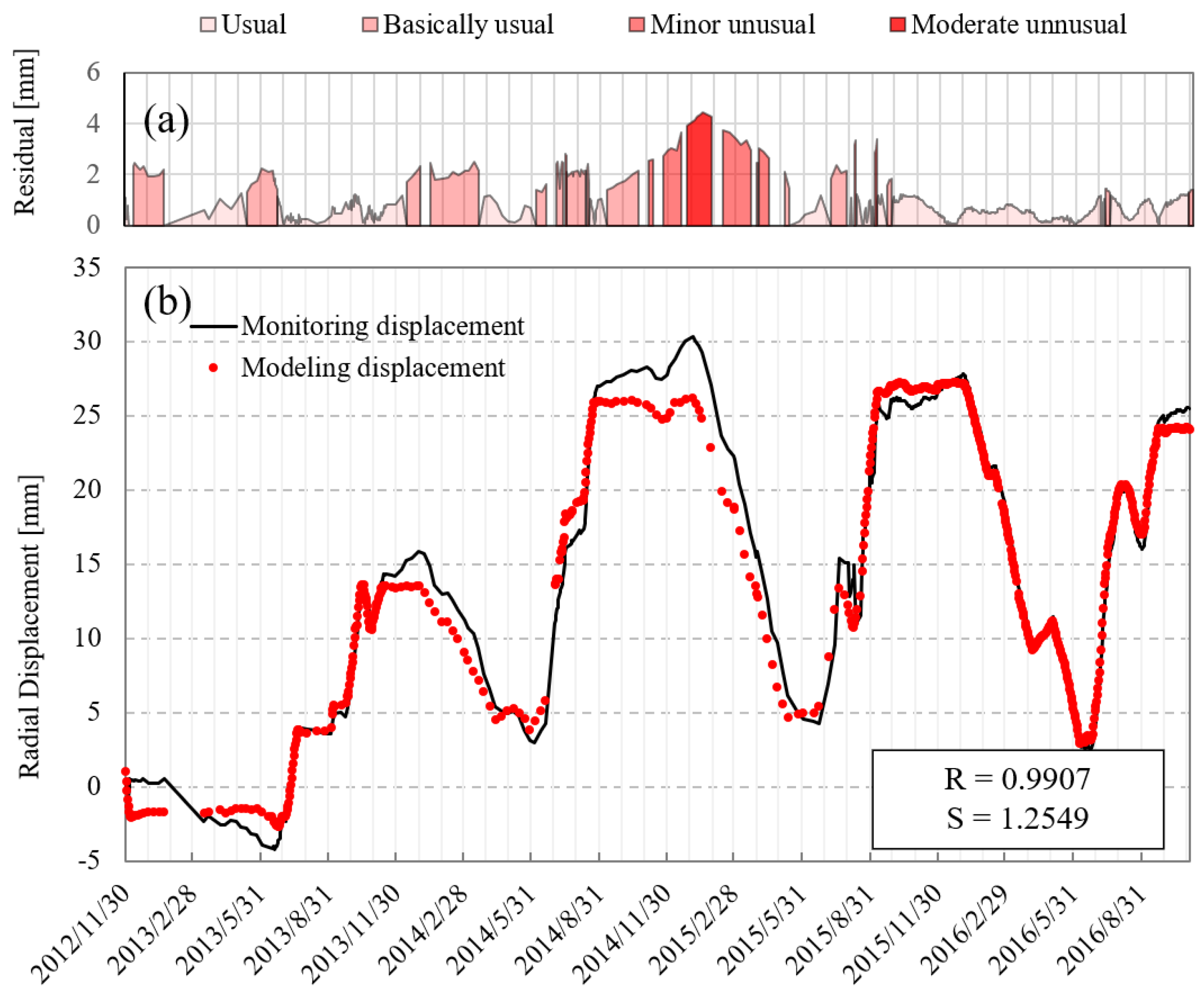
Monitored displacement data reflect a dam’s real-time structural behaviour and can be easily acquired, benefiting from the widely installed monitoring instruments inside the dam. Modelled displacement data, which are estimated from related parameters of the external environment (e.g., upstream water level, temperature), imply the theoretical dam displacement. To assess the dam risk, we established a risk ratio function based on the distribution of residual between the monitored and modelled displacement data. For an arch concrete dam (e.g., the selected dam in the present study), the radial displacement is commonly used to evaluate the risk to dam safety.
A statistical model is commonly used to obtain the radial modelled displacement data δ ^ . In the statistical model, the dam’s radial displacement consists of three components—a water pressure component δ H , a temperature component δ T and an aging component δ θ . The modelled displacement data δ ^ can be expressed as:
δ ^ = δ H + δ T + δ θ
The water pressure component δ H is the sum of the displacement of the dam body itself δ 1 H , the dam foundation δ 2 H and the dam bedrock’s rotational displacement δ 3 H under the upstream water load. δ 1 H , δ 2 H and δ 3 H are as functions of the upstream water level H.
δ H = δ 1 H + δ 2 H + δ 3 H
δ 1 H , δ 2 H and δ 3 H 
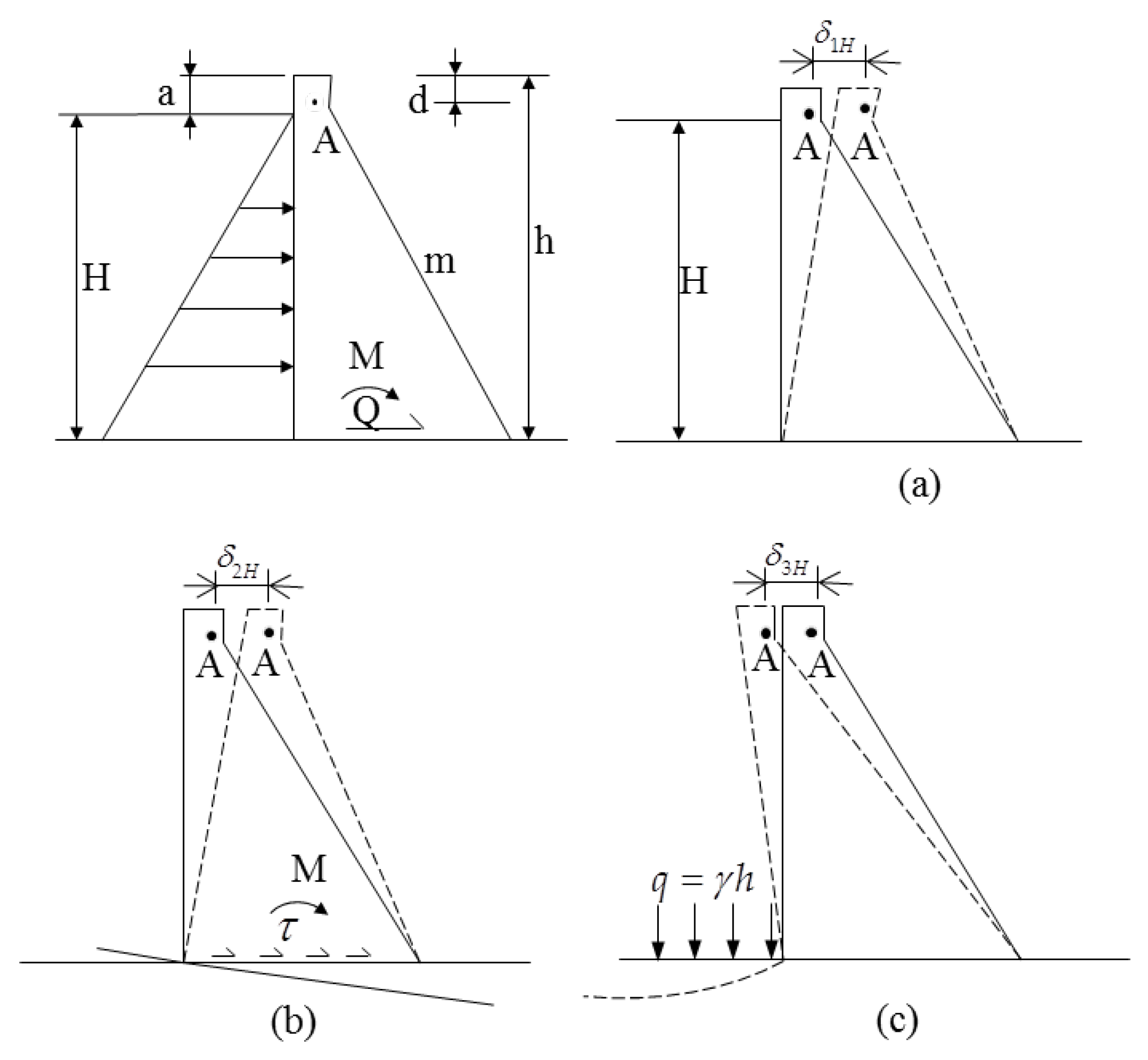
are obtained on the basis of engineering mechanics, which simplifies the gravity dam as a beam structure and the arch dam as an arch shape beam structure. Figure 1 shows a stretch of dam displacement due to water pressure δ H .
Taking the gravity dam as an example,
δ 1 H = γ 0 E c m 3 h d 2 + 6 h H d l n h d + d h + 6 h H 2 d h 1 + d l n h d h H 3 h 2 d h d 2 + γ 0 G c m h 2 d 2 4 h H h d + h H 2 2 l n h d
δ 2 H = 3 1 μ r 2 γ 0 π E r m 2 h 2 H 3 + 1 + μ r 1 2 μ r γ 0 2 E r m h H 2 h d
δ 3 H = α H
Then, for the gravity dam, δ H is written as:
δ H = a 1 H + a 2 H 2 + a 3 H 3
For the arch dam, owing to its more complicated structure, δ H is a polynomial function at least of third order:
δ H = a 1 H + a 2 H 2 + a 3 H 3 +
The coefficients a i are related to the dam height h, downstream slope angle m, the distance from the monitoring point to the dam foundation d and the material parameters including the elastic modulus of the dam body E c , Poisson’s ratio of the dam body μ c , elastic modulus of the foundation E r and Poisson’s ratio of the foundation μ r .
The temperature component δ T is the displacement mainly resulting from internal temperature variation. When the internal monitored temperature data is lacking, researchers often apply a trigonometric function to describe δ T .
δ T = j = 1 2 ( b j 1 s i n ( i d ) + b j 2 c o s ( i d ) )
where d = 2 π t 365 and t is the number of days from the beginning of the monitoring sequence, b j 1 and b j 2 are pending coefficients. Equation (8) is used to describe the temperature effect with one-year or six-month periodicity.
The aging component δ θ characterizes the irreversible displacement caused by the factors such as creep and fatigue of concrete. Due to the difficulties of expressing δ θ theoretically, we provide a formula considering time as a variable to describe its tendency.
δ θ = c 1 θ + c 2 l n θ
where θ is a parameter related to the time of the observation date t and the time of the initial date t 0 , which can be expressed as θ = ( t t 0 ) / 100 ; c 1 and c 2 are pending coefficients.
Then, the statistical model used to model the dam’s displacement can be written as:
δ ^ = i = 1 n a i H i + j = 1 2 b j 1 sin 2 π j t 365 + b j 2 cos 2 π j t 365 + c 1 θ + c 2 l n θ
where n = 3 for gravity dam and n ≥ 4 for arch dam; a i are pending coefficients in the water pressure component δ H , b j 1 and b j 2 are pending coefficients in the temperature component δ T and c i are pending coefficients in the aging component δ θ , which can be estimated by Ordinary Least Squares regression with monitored displacement data δ as test sets. After coefficients are determined, with input sets of upstream water level H and number of days from the beginning of monitoring sequence t, the modelled displacement δ ^ can be calculated.
In practical engineering, the occurrence probability of the event—that the monitored displacement data δ has a large deviation from the modelled displacement data δ ^ —is fairly low. We adopted the occurrence probability of the absolute residual between δ and δ ^ 
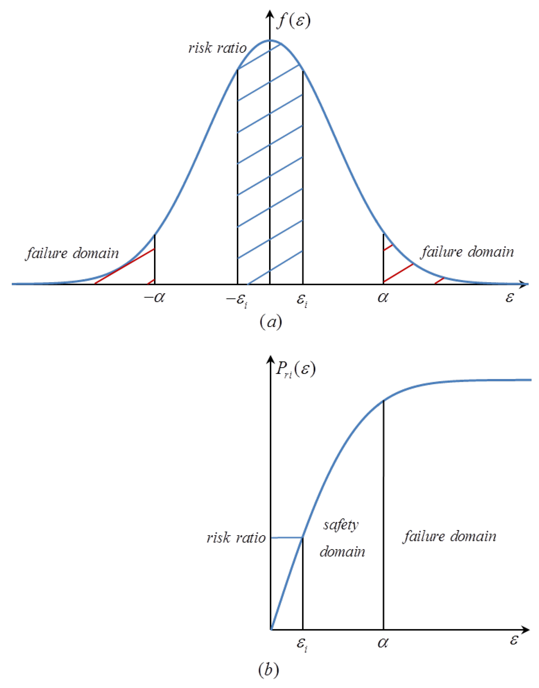
to assess dam risk. Here, we quantified the probability of dam risk by risk ratio and proposed a cumulative distribution function (CDF) of the absolute residual to express it (see Equation (11)).
P | ε | , t = F | X | | ε t | | ε t | < α 1 | ε t | α
where | ε t | = | δ t δ ^ t | is the absolute difference between monitored and modelled displacement data; P | ε | , t denotes the risk ratio; t is time; F | X | | ε t | is the CDF of the absolute residual; α is a failure limit indicator. Figure 2 exhibits the relationship between the risk ratio P and the absolute residual | ε | . The interval of the risk ratio is [0,1]. Based on the small probability method, once | ε | exceeded the limit value α , the monitoring point region would be regarded as being in a failure state.

2.2. Multi-Monitoring Point Risk Ratio Function

With the method presented in Section 2.1, we can obtain the real-time risk ratio P ( | ε | , t ) of a single monitoring point. As both the value of the loading combination and the material resistance are identical for adjacent monitoring points, it is of great importance to take into consideration the correlations of the displacement of adjacent monitoring points. Therefore, we applied a joint CDF to express the risk ratio for multiple monitoring points. The combined risk ratio for multiple monitoring points becomes:
P x 1 , x 2 , , x n ; t = P | X 1 | | ε 1 t | , | X 2 | | ε 2 t , , | X n | | ε n t |
where X i i = 1 , 2 , , n denote the random variables of | ε | of the i-th monitoring point; P x 1 , x 2 , , x n ; t denotes the risk ratio of the dam section. Section 2.2 presents how the joint CDF is constructed by copula functions.

2.2.1. Copula Theory

Sklar (1973) [28] proposed that any joint distribution function can be decomposed into N marginal distribution functions and one copula function, in which the copula function describes the relevance structure between random variables. Here, each single-monitoring point risk ratio function is a marginal distribution function and the multi-monitoring point risk ratio function is the joint distribution function. Hence, the copula function essentially constructs the multi-monitoring point risk ratio function by connecting the risk ratio functions of several monitoring points.
Suppose the joint CDF of the d-dimensional random vector ( X 1 , X 2 , , X d ) is F x 1 , x 2 , , x d , the marginal CDFs are F 1 , F 2 , , F d and C is the copula function that characterizes the correlation between each random vector ( X 1 , X 2 , , X d ) , the joint CDF of the d-dimensional vector ( X 1 , X 2 , , X d ) can be expressed as:
F x 1 , x 2 , , x d = C F 1 x 1 , F 2 x 2 , , F d x d
Then, several commonly used distributions, including Exponential, Gamma, Lognormal and Weibull distributions, were selected as possible marginal distributions of absolute residuals of each displacement data series. The distribution functions of the selected four marginal distributions and the parameters are presented in Table 1.
Three Archimedean copulas (i.e., Clayon copula, Frank copula and Gumbel copula) were used to construct the joint CDFs for a risk ratio of multi-monitoring points. Table 2 shows their generator functions and ranges of related parameters.

2.2.2. Parameters of Distribution Functions Determination

We used the maximum likelihood estimation to estimate the parameters in both marginal distribution functions and copula distribution functions. First, the likelihood function is expressed by:
L θ = i = 1 n c u 1 , u 2 , , u n ; θ = i = 1 n n C u 1 , u 2 , , u n ; θ u 1 u 2 u n
In order to make a simplification, we used the logarithm form of the likelihood function l n L θ in the following calculations (see Equation (15)).
l n L θ = i = 1 n c u 1 , u 2 , , u n ; θ = i = 1 n l n c u 1 , u 2 , , u n
By solving Equation (16), we can obtain that the maximum likelihood estimator θ ^ M L satisfying l n L θ ^ M L l n L θ .
l n L θ θ = 0

2.2.3. Optimal Distribution Function Selection

In order to find the optimal distribution functions, three statistical tests, including Kolmogorov-Smirnov (K-S), root mean square error c(RMSE) and the Akaike information criterion (AIC), were used.
The K-S test evaluates whether the random variables X follow the selected CDF by comparing the samples’ actual distribution F n x and the theoretical distribution of selected CDF F x . The statistics for the K-S test are D n = sup x | F n x F x | and the observation of D n can be defined as:
D ^ n = max 1 k n | F n ( x k ) F ( x k ) | ( k = 1 , 2 , , n )
The D n ( α ) can be obtained, once the significance level α and the sample size n are determined. Then, if D ^ n < D n ( α ) , we may consider that the theoretical distribution of selected CDF F ( x ) fits well with the actual distribution of sample data F n ( x ) ; otherwise, the selected CDF is not matched with the samples.
RMSE reflects the difference between the theoretical probability of selected CDF and the empirical probability of sample data. The equation of RMSE is written as:
R S M E = 1 n i = 1 n [ F c ( i ) P 0 ( i ) ] 2
where n is the sample size, F c is the theoretical probability distribution, P 0 denotes the empirical probability of the sample data.
AIC estimates the relative amount of information lost by the selected CDF, with the consideration of its goodness of fit and simplicity. The AIC is expressed as:
A I C = 2 l n ( L ) + 2 m
where L is the likelihood function of the selected CDF, m is the number of parameters in the selected CDF.
The flowchart of the proposed method is exhibited in Figure 3.

3. Data Sets

In this study, we selected the concrete dam at Jinping-I Hydropower station as an engineering example. The selected dam, with a height of 305 m, is currently the highest concrete arch dam in the world. Figure 4 shows a picture of the selected dam and its location. As the dam adopted the construction form that casting the remaining transverse joints between dam sections, we supposed that the risk probabilities of different dam sections are independent and took monitoring points at one dam section as examples.
Figure 5a represents the distribution map of all 24 displacement monitoring points that were installed inside the dam Sections 5#, 9#, 11#, 13#, 16#, 19#, respectively. In this study, we chose Section 9#, which includes three monitoring points (PL9-3, PL9-4 and PL9-5), as an example. We selected the radial displacement monitored data (to the downstream is positive, to the upstream is negative) from 20 November 2012 to 4 November 2016. The radial displacement was measured twice a day during the flood season and once a day during the drought season and we calculated the average radial displacement for each day. There were 676 validated time frames in total. The time evolution of the radial displacement of the selected three monitoring points, as well as the upstream water level, are exhibited in Figure 5b. It is noticeable that the trend of the radial displacement at the selected three monitoring points had high relevance.

4. Results and Discussion

According to Section 2, we first calculated the modelled displacement data δ ^ ( t ) of these three monitoring points by Equation (10) using the Ordinary least square regression. We then determined the absolute residual between modelled and monitored displacement data | ε t | = | δ t δ ^ t | . With the absolute residual | ε | , we constructed a risk ratio function for each monitoring point. Then, with the optimal marginal distribution of each random variable, we applied copula functions to construct the joint distribution function, so as to determine the risk ratio of the whole dam section.

4.1. Single-Point Qualitative Risk Assessment

First, we determined the modelled displacement data δ ^ i using a statistical model (Section 2.1) for each monitoring point and compared them with the monitored displacement data δ . Time variation of the δ ^ i and δ i of the monitoring points PL9-3, PL9-4 and PL9-5 are shown in Figure 6a, Figure 7a and Figure 8a, respectively. Then, we calculated the absolute residual | ε i | between the δ ^ i and δ i . In many earlier studies, the dam’s running status risk was qualitatively analysed based on the classification of the absolute residual | ε i | with a building assessment index system [29]. We adopted s (standard deviation) to set the borders of the intervals. Standard deviation is used to describe the dispersion degree in the sample and we considered that if the residual obeys a normal distribution, then the proportion of the residual belonging to interval [0, s), [s, 2s), [2s, 3s) and [3s, +∞) are 68.3%, 27.3%, 4.2% and 0.2%, respectively. According to the quantitative description and assessment intervals on the evaluation index, the original information of the evaluation indexes are classified into different divided evaluation levels. Here, the intervals on the evaluation index and the evaluation level of the dam’s risk are divided as follows:
| ε i | = | δ i δ ^ i | = [ 0 , s ) Usual [ s , 2 s ) Basically usual [ 2 s , 3 s ) Minor unusual [ 3 s , + ) Moderate unusual
To avoid the human effect, here we classified the dam’s risk into 4 groups based on the probability of the occurrence of the residual between the monitored and modelled data. A higher residual means a higher level of risk; however, the exact value for the risk of dam collapse needs further simulation based on mechanics. The occurrence probability of the ‘moderate unusual’ group is 0.2% but the risk of dam collapse is a lot lower than 0.2%. The objective of the classification of risk is to provide a quantitative criterion for engineers to determine the frequency of measurement (e.g., whether the dam requires additional measurement). The present study set the interval using s, 2 s and 3 s but these intervals are not absolute. Table 3 presents the frequency of monitoring response to each interval of level of risk.
Figure 6a, Figure 7a and Figure 8a exhibit the absolute residuals of these three monitoring points and the shades of red represent different risk descriptions.
The correlation coefficient R of monitoring points PL9-3, PL9-4 and PL9-5 are 0.9907, 0.9954 and 0.9910, respectively. The R for all the monitoring points is above 0.9, which means the modelling results using the statistical model are good. It is striking from Figure 6, Figure 7 and Figure 8 that each monitoring point had a period in which the monitored displacement value was moderately unusual. PL9-3 was in moderate unusual status from 29 December 2014 to 29 January 2015 (32 days); PL9-4 was in moderate unusual status from 12 January 2015 to 28 April 2015 (107 days); PL9-5 was in moderate unusual status from 1 April 2015 to 12 May 2015 (42 days). Qualitative risk assessment can be used in concrete dam management. However, applications based on qualitative results are limited, as risk comparisons among different monitoring points cannot be achieved. From Section 4.2, Section 4.3, Section 4.4 and Section 4.5, the risk ratio considering the correlation between each monitoring point is calculated for quantitative risk assessment.

4.2. Correlations between Monitoring Points

In order to determine the strength of the relevance of selected monitoring points, we first evaluated the coefficient of correlation between absolute residuals of each monitoring point ( | ε | 9 3 , | ε | 9 4 and | ε | 9 5 ) ). Using a Pearson correlation coefficient (Equation (21)), the correlation between each random variable is represented in Figure 9.
r x y = i = 1 n ( X i X ¯ ) ( Y i Y ¯ ) i = 1 n ( X i X ¯ ) 2 I = 1 N ( Y i Y ¯ ) 2
where r x y is the Pearson correlation coefficient, X i and Y i are random variable pairs of | ε i | (i.e., PL9-3 and PL9-4, PL9-4 and PL9-5, or PL9-5 and PL9-3).
As can be seen from Figure 9, the correlations between these three pairs of variables are quite significant. Especially, the Person correlation coefficient r between | ε | 9 3 and | ε | 9 4 is as high as 0.84. The lowest one is 0.62 between | ε | 9 3 and | ε | 9 5 , which also represents a high correlation.
In addition to the Person correlation coefficient, the Spearman’s rank correlation coefficient (Equation (22)–(23)) and the Kendall’s rank correlation coefficient(Equation (24)–(25)) were also calculated. The correlations between each pair of random variables are represented in Table 4.
ρ n = i = 1 n ( R i R ¯ ) ( S i S ¯ ) i = 1 n ( R i R ¯ ) 2 I = 1 N ( S i S ¯ ) 2
R ¯ = 1 n i = 1 n R i = n + 1 2 = 1 n i = 1 n S i = S ¯
where ρ n is Spearman’s rank correlation coefficient; R i and S i are ranks of random variables X and Y, respectively.
τ = 2 n ( n 1 ) 1 < j n s i g n [ ( x i x j ) ( y i y j ) ]
where τ is the Kendall rank correlation coefficient; n is the sample size; ( x i , y i ) are the pairs of random variables; s i g n ( · ) is the sign function which satisfies:
s i g n ( · ) = 1 ( x i x j ) ( y i y j ) > 0 1 ( x i x j ) ( y i y j ) < 0 0 ( x i x j ) ( y i y j ) = 0
According to Table 4, correlation coefficients of | ε 9 3 | , | ε 9 4 | and | ε 9 5 | are all more than zero, which means a positive relevance between | ε 9 3 | and | ε 9 4 | , | ε 9 4 | and | ε 9 5 | , | ε 9 3 | and | ε 9 5 | .

4.3. Marginal Distributions

To determine a best fitted marginal distribution for the random variables, we first selected four commonly used distribution functions—Exponent function, Gamma function, Lognormal function and Weibull function. Then, we adopted a Maximum Likelihood Estimate to estimate the parameters in each selected marginal distribution (see Section 2.2.1). Table 5 exhibits the estimated parameters and the results of statistical tests for selected distribution functions and random variables. The values of the K-S test did not exceed their critical values 0.05 and D 30 ( 0.05 ) = 0.409 , which implies that all empirical distributions fitted well with the marginal distributions for | ε | 9 3 , | ε | 9 4 and | ε | 9 5 . The CDF fitting curves of the selected four distribution functions for | ε | 9 3 , | ε | 9 4 and | ε | 9 5 are shown in Figure 10, Figure 11, Figure 12 and Figure 13. It is surprising that the Gamma distribution had the lowest RMSE and AIC for | ε | of all three of these monitoring points; hence, it was selected as the preferred marginal distribution to establish a joint probability model.

4.4. Copula-Based Multivariate Joint Distributions

We used three Archimedean copulas including Clayon, Frank and Gumbel to connect the marginal distributions of | ε | 9 3 , | ε | 9 4 and | ε | 9 5 . First, we compared the theoretical probabilities of the Archimedean copulas and the empirical probabilities of sample data. As shown in Figure 14, Figure 15 and Figure 16, the plots of all copulas have a deviation from the 45 diagonal line. For the first impression, the minimum deviation from diagonal line were with the Gumbel copula, which implies that the Gumbel is the best suited copula. It should be noted that, when the empirical probability exceeds 0.8, the Gumbel copula starts to overestimate the risk ratio. However, overestimation during a high level of risk improves the safety of risk management. In contrast, Clayon and Frank copulas overestimate the risk ratio when the empirical probabilities are below 0.4; however, they underestimate the probabilities when they exceed 0.4.
In addition, we calculated the statistical tests of these three copula functions and find the same results as with the comparison of probabilities. Table 6 exhibits the copula parameters θ as well as the results of statistical tests RSME and D n for each joint distribution function. The Gumbel distribution was selected as the optimal joint distribution for multiple variables, as it has the lowest RSME of 0.0285 and the lowest D n of 0.0711.

4.5. Multi-Point Risk Ratio

In this section, we constructed a joint distribution based on the risk ratio of each monitoring point with the Gumbel copula, which represents the occurrence probability of the event ( X 1 | ε | 1 , X 2 | ε | 2 , X 3 | ε | 3 ) . 0.95 was the assessment criterion of the joint distribution probability—once the joint distribution probability exceeds 0.95, the running status of the selected dam section will be regarded as moderately unusual.
According to the method in Section 2.1, the risk ratios of these three monitoring points are calculated, respectively. Figure 17 shows the time evolution of risk ratios of these three monitoring points. Each monitoring point has different probabilities of moderate–unusual running status.
As can be seen from Figure 17, the risk ratios of the three monitoring points varied sharply during the whole period (from 20 November 2012 to 4 November 2016), while the average values are quite close, being 0.4961, 0.4927 and 0.4975, respectively. Then, we calculated the risk ratios in the most recent year (from January 1 2016 to November 1 2016), the average values being 0.3925, 0.3965 and 0.4329, respectively. By comparison of these risk ratios, we discovered that the risk ratios surrounding the monitoring point PL9-5 in dam Section 9# are relatively high. Therefore, attention should be paid to safety inspection around the dam foundation region.
Figure 18 represents the multi-point risk ratios calculated with subjective weight method (setting even weight as 0.333 for PL9-3, PL9-4 and PL9-5 without the consideration of correlations) and multivariate copulas. The results obtained by the proposed method have a similar tendency to the subjective weight method. Taking account of the structural correlation, the risk ratios with multivariate copulas were above 0.95 from 29 December 2014 to 15 March 2015 and from 1 April 2015 to 14 April 2015, which implies the dam section was in moderate–unusual status during those periods. The evaluated time of moderate–unusual running status was 45 days less than that without considering the correlations, namely, the previous methods overestimated the probability of risk.
Multivariate copulas construct the joint distribution to describe the occurrence probability of the event ( X 1 | ε | 1 , X 2 | ε | 2 , X 3 | ε | 3 ) , which considers the running status of these three monitoring points simultaneously. In this way, the description of the running status of one dam section is more practical, as all components in the dam section are considered to be bearing external loads (upstream water pressure and temperature changes) as an integral structure. In addition, the multivariate copulas method expresses the correlations merely on the basis of displacement monitoring data, which is objective. Therefore the multi-point risk ratio of the proposed method was more rational to use for risk assessment.

5. Conclusions

The present study proposed a data-driven method based on multivariate copulas for the risk assessment of a dam’s safety, with the objective of assessing the dam risk quantitatively and to consider the correlation of displacement between each monitoring point. The concrete dam at Jinping-I Hydropower Station was selected as a case study. We first calculated the absolute residuals between monitored and modelled displacement data for a single monitoring point. We then used multivariate copulas to connect the distribution functions of different monitoring points. The Gamma distribution was selected as the optimal marginal distribution. Gumbel copula, which fitted best with the empirical probabilities, was selected as the joint distribution. Considering that the risk probabilities of different dam sections are independent, we took one dam section, which includes three monitoring points, as an example, and we estimated the real-time running status of the selected dam section, which we call the risk ratio. The risk ratio helps us to explain and quantify the level of the dam’s safety and the measurement frequency needs. The following conclusions are remarkable:
First, the risk ratio of each monitoring point was highly dependent on its displacement and the residual between monitored and modelled displacement data; the risk ratio of the selected dam section had a slight deviation from the risk ratios of each monitoring point.
Second, taking account of the temporal and spatial correlations among the selected monitoring points with a Copula function, the estimated moderate unusual time was 45 days less than that without considering the correlations. This means that the previous methods overestimated the probability of risk. Most previous studies considered displacement at different monitoring points as independent variables and assessed the risk for each monitored point separately.
In addition, the risk ratios during flood seasons were slightly higher than those during drought seasons, indicating that monitoring frequency should be increased during flood seasons. The risk ratio can provide a quantitative indicator for the measures management of the dams.

Author Contributions

Conceptualization, C.S.; methodology, C.S., Y.H.; validation, Y.H., C.S. and Z.M.; formal analysis, Y.H., C.S., C.G.; data curation, Y.H. and Z.M.; writing—original draft preparation, C.S.; writing—review and editing, Y.H. and Z.M.; supervision, C.G.

Funding

The research was funded by National Natural Science Foundation of China (Grant Nos. 51739003, 51579085, 51779086, 51579086, 51379068, 51579083, 51609074), National Key R&D Program of China (2018YFC0407104, 2018YFC1508603, 2018YFC0407101, 2016YFC0401601), Project Funded by the Priority Academic Program Development of Jiangsu Higher Education Institutions (YS11001), Special Project Funded of National Key Laboratory(20165042112), Key R&D Program of Guangxi (AB17195074).

Conflicts of Interest

The authors declare no conflict of interest.

Abbreviations

The following abbreviations are used in this manuscript:
AICAkaike Information Criterion
CDFCumulative Distribution Function
K-SKolmogorov-Smirnov
RSMERoot Mean Square Error

References

  1. Spouge, J. A Guide to Quantitative Risk Assessment for Offshore Installations; CMPT: Aberdeen, Scotland, 1999. [Google Scholar]
  2. Liang, R.; Nusier, O.; Malkawi, A. A reliability based approach for evaluating the slope stability of embankment dams. Eng. Geol. 1999, 54, 271–285. [Google Scholar] [CrossRef]
  3. Sivakumar Babu, G.; Srivastava, A. Reliability analysis of earth dams. J. Geotech. Geoenviron. Eng. 2010, 136, 995–998. [Google Scholar] [CrossRef]
  4. Altarejos-García, L.; Escuder-Bueno, I.; Serrano-Lombillo, A.; de Membrillera-Ortuño, M.G. Methodology for estimating the probability of failure by sliding in concrete gravity dams in the context of risk analysis. Struct. Saf. 2012, 36, 1–13. [Google Scholar] [CrossRef]
  5. Wu, Z. Safety Monitoring Theory and Its Application of Hydraulic Structures; Higher Education: Beijing, China, 2003. [Google Scholar]
  6. Salazar, F.; Morán, R.; Toledo, M.Á.; Oñate, E. Data-based models for the prediction of dam behaviour: A review and some methodological considerations. Arch. Comput. Methods Eng. 2017, 24, 1–21. [Google Scholar] [CrossRef]
  7. Seker, D.; Kabdasli, S.; Rudvan, B. Risk assessment of a dam-break using GIS technology. Water Sci. Technol. 2003, 48, 89–95. [Google Scholar] [CrossRef] [Green Version]
  8. Salgueiro, A.R.; Pereira, H.G.; Rico, M.T.; Benito, G.; Díez-Herreo, A. Application of correspondence analysis in the assessment of mine tailings dam breakage risk in the Mediterranean region. Risk Anal. Int. J. 2008, 28, 13–23. [Google Scholar] [CrossRef]
  9. Zhong, D.; Sun, Y.; Li, M. Dam break threshold value and risk probability assessment for an earth dam. Nat. Hazards 2011, 59, 129–147. [Google Scholar] [CrossRef]
  10. Chauhan, S.S.; Bowles, D.S. Dam safety risk assessment with uncertainty analysis. Ancold Bull. 2004, 127, 73–88. [Google Scholar]
  11. Wu, Z.; Su, H. Dam health diagnosis and evaluation. Smart Mater. Struct. 2005, 14, S130. [Google Scholar] [CrossRef]
  12. Shao, C.; Gu, C.; Yang, M.; Xu, Y.; Su, H. A novel model of dam displacement based on panel data. Struct. Control. Health Monit. 2018, 25, e2037. [Google Scholar] [CrossRef]
  13. Hu, Y.; Shao, C.; Gu, C.; Meng, Z. Concrete Dam Displacement Prediction Based on an ISODATA-GMM Clustering and Random Coefficient Model. Water 2019, 11, 714. [Google Scholar] [CrossRef]
  14. Samaras, G.D.; Gkanas, N.I.; Vitsa, K.C. Assessing risk in dam projects using AHP and ELECTRE I. Int. J. Constr. Manag. 2014, 14, 255–266. [Google Scholar] [CrossRef]
  15. Qin, X.; Gu, C.; Zhao, E.; Chen, B.; Yu, Y.; Dai, B. Monitoring indexes of concrete dam based on correlation and discreteness of multi-point displacements. PLoS ONE 2018, 13, e0200679. [Google Scholar] [CrossRef] [PubMed]
  16. Wu, Z.; Su, H.; Guo, H. Assessment model of dam operation risk based on monitoring data. Sci. China Ser. E Technol. Sci. 2007, 50, 144–152. [Google Scholar] [CrossRef]
  17. Frees, E.W.; Valdez, E.A. Understanding relationships using copulas. North Am. Actuar. J. 1998, 2, 1–25. [Google Scholar] [CrossRef]
  18. Jaworski, P.; Durante, F.; Hardle, W.K.; Rychlik, T. Copula Theory and Its Applications; Springer: Berlin/Heidelberg, Germany, 2010; Volume 198. [Google Scholar]
  19. Salvadori, G.; De Michele, C. Frequency analysis via copulas: Theoretical aspects and applications to hydrological events. Water Resour. Res. 2004, 40. [Google Scholar] [CrossRef]
  20. Klein, B.; Schumann, A.H.; Pahlow, M. Copulas—New Risk Assessment Methodology for Dam Safety. In Flood Risk Assessment and Management; Springer: Dordrecht, The Netherlands, 2011; pp. 149–185. [Google Scholar]
  21. Savu, C.; Trede, M. Hierarchies of Archimedean copulas. Quant. Financ. 2010, 10, 295–304. [Google Scholar] [CrossRef]
  22. Demarta, S.; McNeil, A.J. The t copula and related copulas. Int. Stat. Rev. 2005, 73, 111–129. [Google Scholar] [CrossRef]
  23. Singh, V.P.; Zhang, L. IDF curves using the Frank Archimedean copula. J. Hydrol. Eng. 2007, 12, 651–662. [Google Scholar] [CrossRef]
  24. Kole, E.; Koedijk, K.; Verbeek, M. Selecting copulas for risk management. J. Bank. Financ. 2007, 31, 2405–2423. [Google Scholar] [CrossRef] [Green Version]
  25. Durrleman, V.; Nikeghbali, A.; Roncalli, T. Which copula is the right one? SSRN Electron. J. 2000, 1–19. [Google Scholar] [CrossRef]
  26. Léger, P.; Leclerc, M. Hydrostatic, temperature, time-displacement model for concrete dams. J. Eng. Mech. 2007, 133, 267–277. [Google Scholar] [CrossRef]
  27. Bui, K.T.T.; Bui, D.T.; Zou, J.; Van Doan, C.; Revhaug, I. A novel hybrid artificial intelligent approach based on neural fuzzy inference model and particle swarm optimization for horizontal displacement modeling of hydropower dam. Neural Comput. Appl. 2018, 29, 1495–1506. [Google Scholar] [CrossRef]
  28. Sklar, A. Random variables, joint distribution functions, and copulas. Kybernetika 1973, 9, 449–460. [Google Scholar]
  29. Su, H.; Wen, Z.; Sun, X.; Yan, X. Multisource information fusion-based approach diagnosing structural behavior of dam engineering. Struct. Control. Health Monit. 2018, 25, e2073. [Google Scholar] [CrossRef]
Figure 1. The three components of δ H : (a) δ 1 H , (b) δ 2 H and (c) δ 3 H .
Jmse 07 00353 g001
Figure 2. The relationship between the risk ratio P and the absolute residual | ε | : (a) the probability density function of | ε | , (b) the risk ratio function based on | ε | .
Jmse 07 00353 g002
Figure 3. Flowchart of the proposed method.
Jmse 07 00353 g003
Figure 4. Picture of the selected concrete arch dam and its location.
Jmse 07 00353 g004
Figure 5. (a) Distribution of the monitoring points from upstream side view; (b) Time variation of radial monitored displacement data at the three selected monitoring points and upstream water level data.
Jmse 07 00353 g005
Figure 6. Time variation of (a) absolute residual and (b) modelled and monitored displacement data for the monitoring point PL9-3.
Jmse 07 00353 g006
Figure 7. Time variation of (a) absolute residual and (b) modelled and monitored displacement data for the monitoring point PL9-4.
Jmse 07 00353 g007
Figure 8. Time variation of (a) classified residual and (b) modelled and monitored displacement data for the monitoring point PL9-5.
Jmse 07 00353 g008
Figure 9. Pearson correlation coefficient r between | ε | 9 3 , | ε | 9 4 and | ε | 9 5 .
Jmse 07 00353 g009
Figure 10. Univariate cumulative distribution function (CDF) fitting curves of | ε | 9 3 : (a) Exponential distribution function, (b) Gamma distribution function, (c) Lognormal distribution function, (d) Weibull distribution function.
Jmse 07 00353 g010
Figure 11. Univariate CDF fitting curves of | ε | 9 4 : (a) Exponential distribution function, (b) Gamma distribution function, (c) Lognormal distribution function, (d) Weibull distribution function.
Jmse 07 00353 g011
Figure 12. Univariate CDF fitting curves of | ε | 9 5 : (a) Exponential distribution function, (b) Gamma distribution function, (c) Lognormal distribution function, (d) Weibull distribution function.
Jmse 07 00353 g012
Figure 13. Univariate PDF fitting curves of (a) | ε | 9 3 , (b) | ε | 9 4 and (c) | ε | 9 5 .
Jmse 07 00353 g013
Figure 14. Comparison of theoretical and empirical probability with Clayon copula: (a) Q-Q plots; (b) empirical and theoretical probabilities.
Jmse 07 00353 g014
Figure 15. Comparison of theoretical and empirical probability with Frank copula: (a) Q-Q plots; (b) empirical and theoretical probabilities.
Jmse 07 00353 g015
Figure 16. Comparison of theoretical and empirical probability with Gumbel copula: (a) Q-Q plots; (b) empirical and theoretical probabilities.
Jmse 07 00353 g016
Figure 17. Displacement risk ratios for monitoring points PL9-3, PL9-4 and PL9-5.
Jmse 07 00353 g017
Figure 18. Multi-point risk ratios for dam Section 9# of the Jinping-I arch dam.
Jmse 07 00353 g018
Table 1. List of the selected marginal distribution functions and parameters.
DistributionCumulative DistributionParameters
Exponential 1 e x δ 1 δ 1
Gamma 1 δ 2 δ 1 Γ ( δ 1 ) x δ 1 1 e x δ 2 δ 1 , δ 2
Lognormal 1 x δ 2 2 π e ( l o g x δ 1 ) 2 2 δ 2 2 δ 1 , δ 2
Weibull δ 2 δ 1 ( x δ 1 ) δ 2 1 e ( x δ 1 ) δ 2 δ 1 , δ 2
Table 2. Generator functions and parameter ranges of selected Archimedean copulas.
NO.NameGenerator FunctionParameter Range
1Clayton 1 θ t θ 1 ( 0 , )
2Gumbel ( l o g ( t ) ) θ [ 1 , ]
3Frank l o g e θ t 1 e θ 1 ( , + ) \ 0
Table 3. Management of monitoring frequency.
State DescriptionsMonitoring Frequency
Usual1 time monitoring per day
Basically usual2–3 times monitoring per day
Minor unusual3–4 times monitoring per day, and one on-site inspection per day
Moderate unusual3–4 times monitoring per day, on-site inspections twice per day and report to Monitoring Management Center
Table 4. Correlations between each pair of random variables.
Correlation IndexSpearman ρ n Kendall τ Pearson r xy
PL9-3 and PL9-40.81380.64020.8357
PL9-4 and PL9-50.68270.54460.6517
PL9-3 and PL9-50.63180.47240.6240
Table 5. Estimated parameters in the marginal distributions and results of statistical tests.
DistributionEstimated ParametersStatistical Tests
PAPB D ^ n D ^ n ( 0.05 ) RMSEAIC
| ε | 9 3 Exponent0.9537-0.09000.4090.03251289.872
Gamma1.42160.67090.03510.01601245.576
Lognormal−0.43870.99040.07020.03291315.256
Weibull1.01991.21720.04290.01871251.53
| ε | 9 4 Exponent0.4730-0.04860.4090.0244341.732
Gamma1.2450.37990.05190.0214324.738
Lognormal−1.20141.05680.07090.0288371.89
Weibull0.49331.11410.05630.0232330.736
| ε | 9 5 Exponent0.2391-0.02340.4090.0090−580.618
Gamma1.22830.19470.02240.0086−595.448
Lognormal−1.89031.11470.04360.0242−487.484
Weibull0.24901.11060.02630.0101−591.056
Table 6. Estimated parameters and statistical test results of the joint distribution.
Archimedean CopulaParametersStatistical Tests
θ RSME D n
Clayon4.230.05230.1043
Frank8.360.03400.0864
Gumbel3.000.02850.0711

