1. Introduction
Impulse waves are generated by very rapid gravity-driven mass movements including landslides and avalanches impacting a body of water (Heller et al. [
1]). The slide energy is transferred to the water column and a wave train is generated, which propagates away from the impact location. Especially water bodies with steep shorelines, e.g., fjords, mountain lakes or reservoirs, are prone to this tsunami-like hazard. Roberts et al. [
2] compiled a global catalogue with 254 landslide-generated impulse wave events. In the past, extreme absolute impulse wave runup heights were observed in Lituya Bay, USA, in 1958 with 524 m (Miller [
3]), Chehalis Lake, Canada, in 2007 with 38 m (Roberts et al. [
4]), and Taan Fjord, USA, in 2015 with 193 m (Higman et al. [
5]).
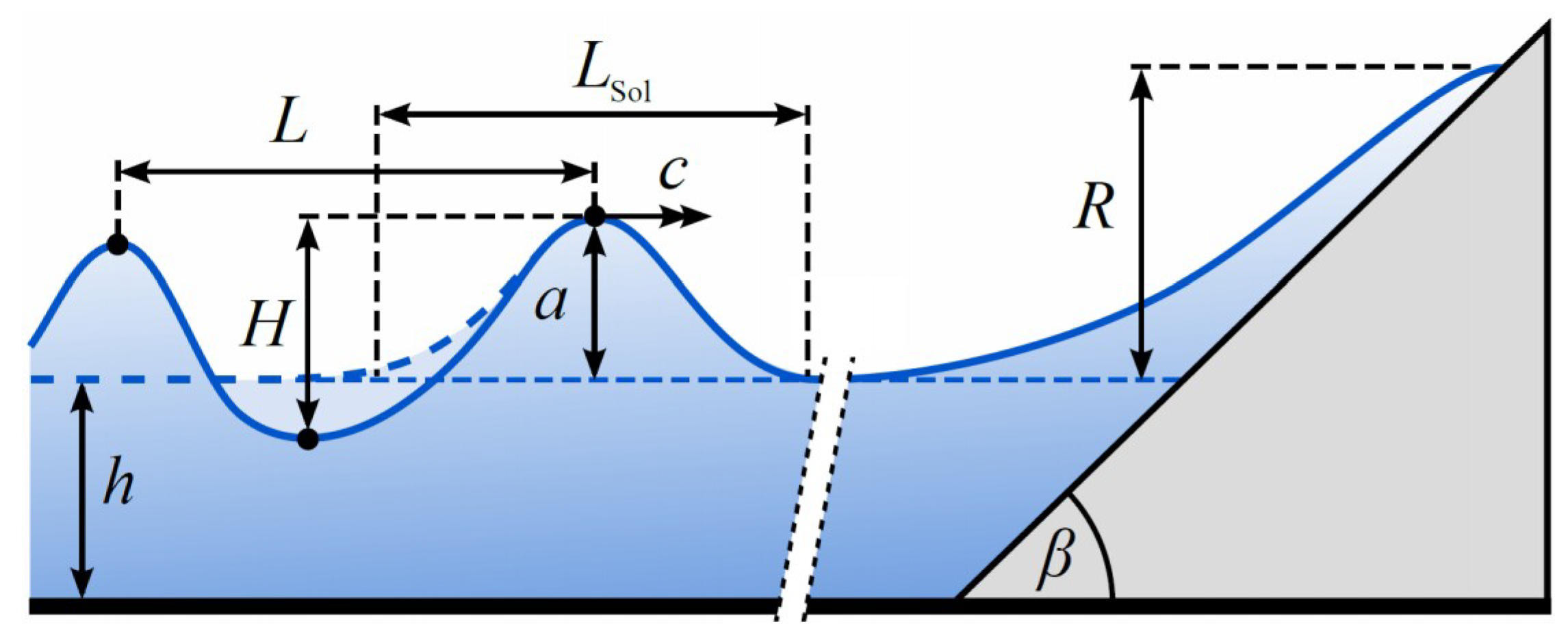
For hazard mitigation, the runup height
R is of primary interest (
Figure 1). While the impulse wave events given above are extreme cases, comparably small runup heights at densely populated lake shores may already cause substantial damage (Fuchs and Boes [
6]). Particularly in reservoirs, where there is a freeboard of just a few meters between the stillwater level and the dam crest, the prediction of runup by small impulse wave amplitudes needs to be as accurate as possible to prevent overtopping. Müller [
7] conducted experiments specifically designed to study the runup of impulse waves and derived an empirical prediction equation for the runup height induced by the first or leading wave, respectively, of the impulse wave train. However, also equations derived from experiments with solitary waves are commonly applied to predict runup heights by impulse waves (e.g., Bregoli et al. [
8], McFall and Fritz [
9]). While a solitary wave features a single wave crest, impulse waves are characterized by an outgoing wave train with multiple wave crests and troughs (
Figure 1).
This study focuses on non-breaking impulse wave runup on steep slopes, i.e., slope angles
β ≥ 10° (
Figure 1). First, runup equations from the literature are discussed. Since there is a multitude of studies on solitary wave runup on gentle slopes (Pujara et al. [
10], Hafsteinsson et al. [
11]), only equations derived from experiments with
β ≥ 10° or those commonly applied for this parameter range are included. A dataset consisting of measured runup heights from both impulse wave and solitary wave (index Sol) runup experiments with
β between 10° and 90° (vertical wall) is then compiled from published experimental data. Subsequently, the runup equations are applied to these data for runup prediction. Based on this comparison, a semi-empirical runup equation is proposed. The discussion includes the limitations of this equation and assesses the significance of scale effects.
2. Runup Equations
The governing parameters included in the prediction equations for the runup height described below are: wave crest amplitude
a, wave height
H, wave length
L, stillwater depth
h, and runup slope angle
β (
Figure 1). While
H is a combined parameter of the first wave crest and trough amplitudes for impulse waves,
H =
a for solitary waves. The relative wave crest amplitude is defined as
ε =
a /
h. While the length of a solitary wave is infinite (Dean and Dalrymple [
12]), it may be approximated with
LSol as the effective wave length (Lo et al. [
13]). For empirically derived prediction equations included below, the corresponding datasets are described in the following section.
Müller [
7] approximated the runup height
R of impulse waves based on wave channel experiments with
Equation (1) contains the two governing wave parameters,
H and
L. The last term including
β equals to 1 for 90° and increases for decreasing
β. To predict the runup height of a solitary wave, its effective wave length may be approximated with (Lo et al. [
13])
Hall and Watts [
14] approximated the runup height
R of solitary waves also based on wave channel experiments with
In the original publication, the runup slope angle
β was expressed in radians, whereas its unit is in (°) in Equation (3). Since this equation was derived for solitary wave runup,
ε is included as the single governing wave parameter. Hall and Watts [
14] state the application range for Equation (3) with
β between 12° and 45°. A different equation is given for
β between 5° and 12°. However, the latter will not be considered in the further analysis, while Equation (3) will be applied to runup angles between 10° and 45° for simplification.
As the third empirical runup equation, Fuchs and Hager [
15] approximated the runup height
R of solitary waves in wave channel experiments with
The governing wave parameter is
ε. The runup slope
β is included in a tangent function. As the tangent of
β = 90° is not defined, wave runup at a vertical wall may not be predicted with Equation (4).
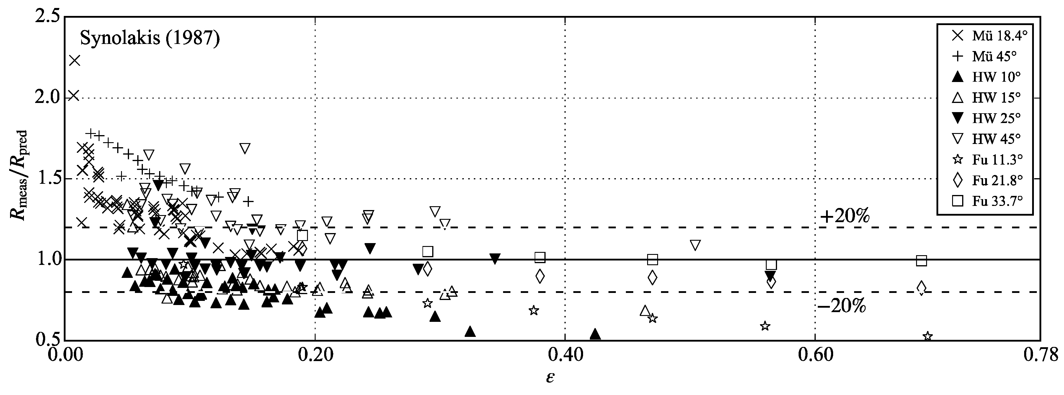
Synolakis [
16] developed an approximate solution of the nonlinear wave theory and applied it to derive an equation describing the maximum runup height
R of a solitary wave with
referred to as
the runup law. Equation (5) is formally correct for
ε0.5 ≫ 0.288 tan
β (Synolakis [
16]). The theoretical approach is compared to own experimental data for a gentle slope with
β ≈ 2.9° (tan
β = 1/19.85) as well as to selected experiments with non-breaking wave runup data by Hall and Watts [
14] with
β between 5° and 45°. Synolakis [
16] finds a satisfactory agreement except for
β = 45°. Similar to Equation (4), the cotangent of
β = 90° equals to zero and therefore wave runup at a vertical wall may not be predicted with Equation (5).
Except for Equation (1), none of the other equations considered runup at a vertical wall, i.e.,
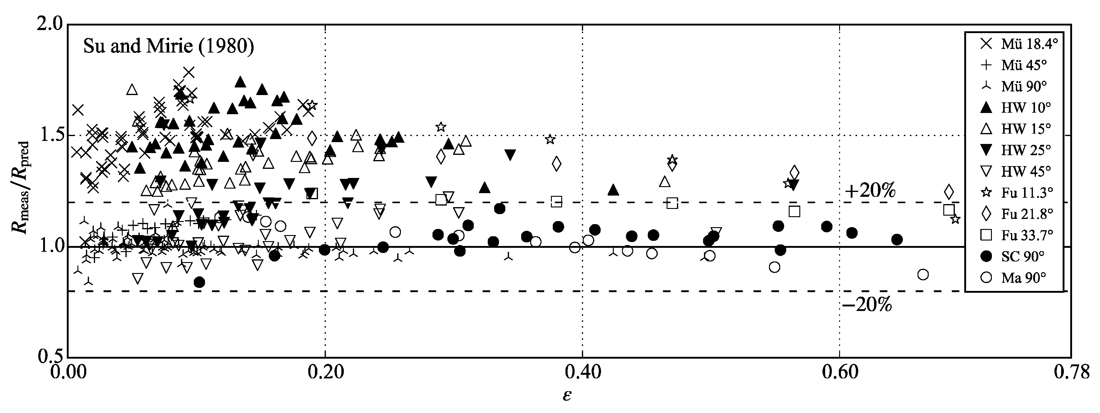
β = 90°. Su and Mirie [
17] studied the collision of two solitary waves and conducted a perturbation analysis of this phenomenon to the third order. If viscosity and surface tension effects are neglected, the case of two colliding solitary waves with the same amplitude is equal to the runup of a single wave at a vertical wall (Cooker et al. [
18]). The maximum runup height
R for
β = 90° is stated by Su and Mirie [
17] with
For very small relative wave amplitudes, the relative runup height
R/
h converges to 2
ε. Maxworthy [
19] presents experimental results for both wave-wave interaction and wave-wall interaction, which indicate that the maximum superposed wave amplitude or runup height, respectively, is approximately 10% higher in the former than in the latter case. However, these experiments were conducted at stillwater depths between 4.5 and 6.7 cm and viscosity as well as surface tension effects might have had a more significant influence compared to larger scales.
3. Datasets
Five experimental datasets were included in the analysis presented herein: Müller [
7] (
n = 166), Hall and Watts [
14] (
n = 138), Fuchs [
20] (
n = 19), Street and Camfield [
21] (
n = 22), and Maxworthy [
19] (
n = 14) with a total of
n = 359 experiments. Their respective key parameter ranges are summarized in
Table 1. In Müller’s [
7] experiments, wave trains with multiple wave crests and troughs were generated to reproduce landslide generated impulse wave characteristics, while the other experimental series document solitary waves, i.e.,
a =
H (
Figure 1). Therefore, the waves generated in the experiments by Müller [
7] will be referred to in the following as
impulse waves, while the remaining are
solitary waves. The generated relative wave amplitudes
ε range from 0.007 to 0.69 and runup slope angles
β from 10° to 90° (vertical wall). While empirical prediction equations were directly derived from the datasets by Müller [
7], Hall and Watts [
14], and Fuchs [
15] as described in the previous section, the data by Street and Camfield [
20] and Maxworthy [
19] for
β = 90° is included to assess the analytically derived Equation (6) by Su and Mirie [
17].
Müller [
7] conducted experiments in a wave channel with a length of 19.25 m, a width of 1 m, and a depth of 1.2 m. The impulse waves were generated by a rectangular box falling vertically onto the water surface at one end of the channel. The box mass ranged from 118 to 422 kg. By adjusting box mass, drop height, and water depth, tests with differing wave characteristics were achieved. Parallel wire wave gauges were applied for measuring the water surface displacement. The installed slope angles
β were 18.4°, 45° and 90°. For tracking the maximum runup height
R of the first wave at the vertical wall (
β = 90°), also wire wave gauges were applied. For the two milder slopes,
R was optically recorded. The accuracy of the wave gauges is given with ±0.1 mm and for the optical method with ±1 to 2 mm. Repeatability tests yielded deviation < 1% for runup heights
R > 40 mm and a larger scatter of 10% for
R < 40 mm.
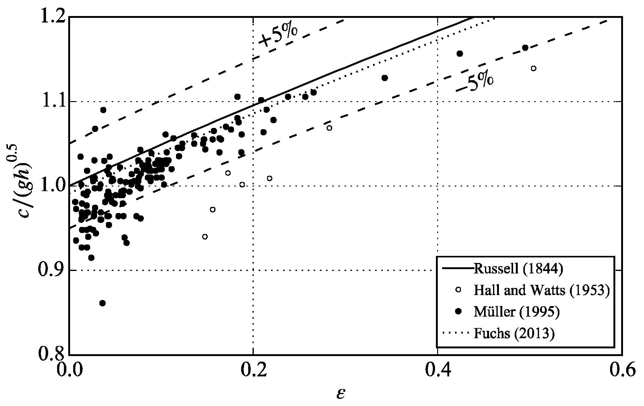
Figure 2 shows the wave crest celerities
c (see
Figure 1) of the first outgoing wave within the impulse wave train as a function of
ε. Compared to the celerity of a solitary wave defined by Russell [
22] as:
the measured impulse wave celerities mainly scatter between 95% and 103% of the solitary wave celerity. This agrees with the findings by McFall and Fritz [
23] and Evers et al. [
24] for spatial impulse wave propagation in wave basins. The relative wave length
L/
h of Müller’s [
7] experiments range between 9 and 56. According to Dean and Dalrymple [
12], the generated waves cover the transition zone from intermediate-water (2 <
L/
h ≤ 20) to shallow-water (
L/
h > 20). The measured wave celerities confirm this classification. In line with the additional text information in Müller [
7], experiments no. 474, 589, 601, and 602 were not included in the analysis. The experiments featuring roughness elements at
β = 18.4° (no. 562–588) were also not considered. All other experiments from Müller’s [
7] appendix providing sufficient information on the impulse wave characteristics as well as the runup height were included in the analysis. The number of experiments included from Müller [
7] is
n = 166 (63 at
β = 18.4°, 17 at
β = 45°, 86 at
β = 90°).
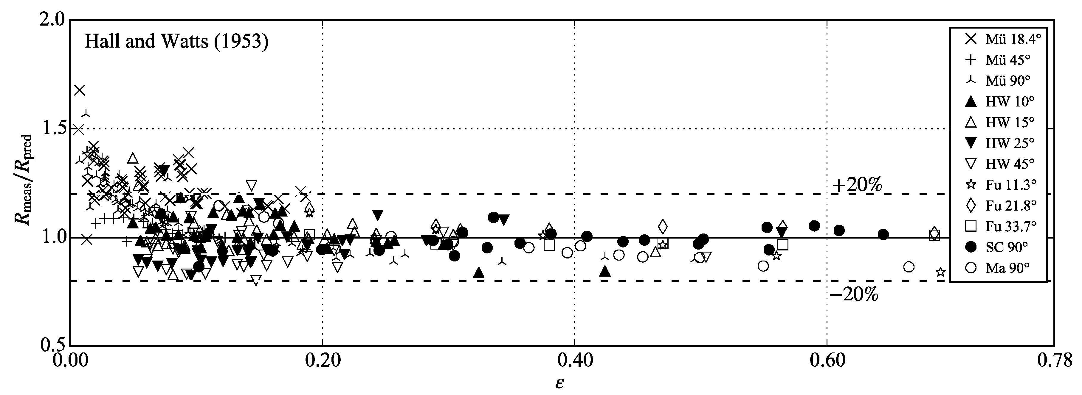
The experiments by Hall and Watts [
14] were conducted in a wave channel with a length of 25.9 m, a width of 4.3 m, and a depth of 1.2 m. The solitary waves were generated with a “pusher type” wave generator featuring a vertical pusher face mounted to a trolley, which was mechanically linked to a gravitationally accelerated drop weight. Both, wave height and runup height were optically measured. Besides slope angles
β = 10°, 15°, 25°, and 45°, also
β = 5° was installed in the channel. However, the latter was not included into this analysis. The measured wave celerities
cSol are within 88% to 94% of Equation (7) (
Figure 2). Two experiments were not included into the analysis for this study as they were quite outside the trend of neighboring data points and therefore classified as obvious outliers (
R/
h = 0.535 and 0.679, both at
β = 10°). The number of experiments included from Hall and Watts [
14] is
n = 138 (38 at
β = 10°, 37 at
β = 15°, 31 at
β = 25°, 32 at
β = 45°).
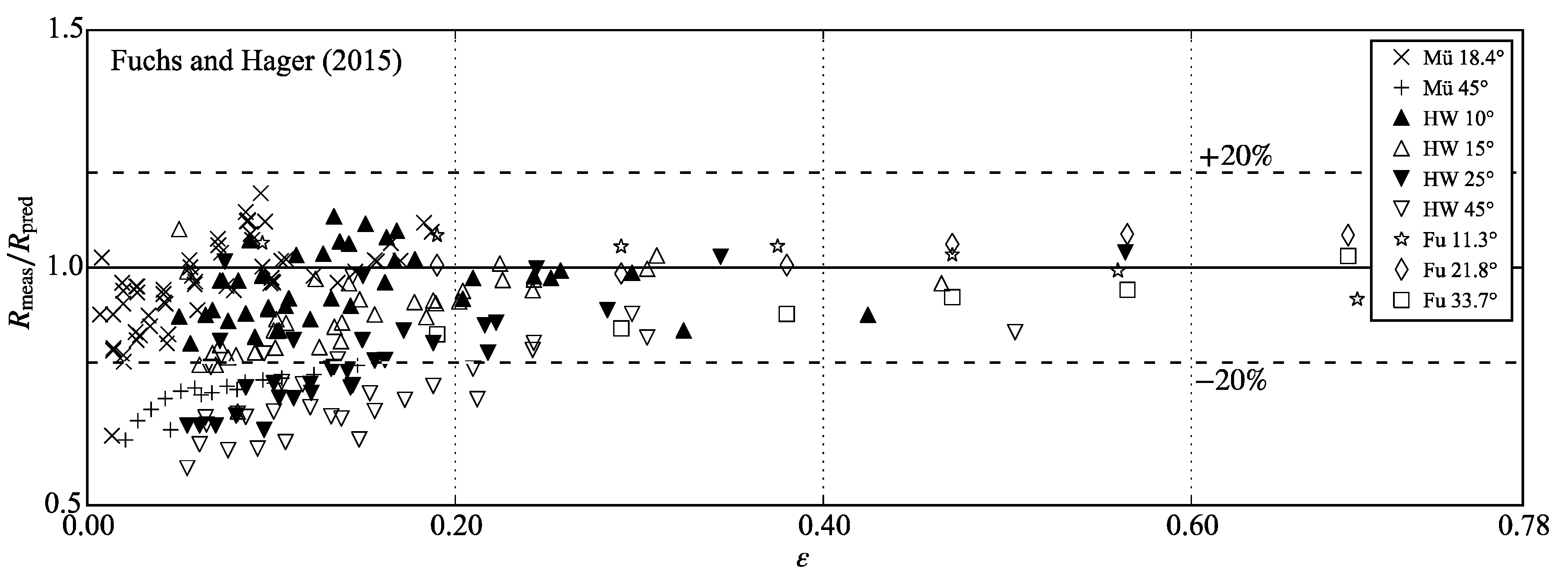
Fuchs [
20] conducted experiments with a pneumatic piston-type wave generator in an 11 m long, 0.5 m wide, and 1 m deep channel. The inclinations of the runup slopes were set to tan
β = 1/5, 1/2.5, and 1/1.5; i.e.,
β ≈ 11.3°, 21.8°, and 33.7°. The solitary wave profiles were tracked with ultrasonic distance sensors and runup heights were measured optically. The measured wave celerities average out at 99.1% of Equation (7) (
Figure 2). The number of experiments included from Fuchs [
20] is
n = 19 (7 at
β = 11.3°, 6 at
β = 22.8°, 6 at
β = 33.6°).
Street and Camfield [
21] studied solitary wave reflection at a vertical wall, i.e.,
β = 90°, in a 17 m long subsection of a channel with a length of 35 m and a width of 0.91 m. The piston-type wave generator was controlled with a hydraulic-servo-electronic system. Wave amplitudes were measured with capacitance wave gauges. Near shore deformation details were optically recorded. The runup data by Street and Camfield [
21] was extracted with WebPlotDigitizer [
25] from the original publication. The number of experiments included from Street and Camfield [
21] is
n = 22.
Maxworthy [
19] studied solitary wave reflection at a vertical wall as well as head-on collision between two solitary waves in a 5 m long, 0.2 m wide, and 0.3 m deep channel. Only runup data at the wall was considered for this study. The waves were generated manually by pulling a plate through the channel. The wave characteristics and the runup height were measured optically. The runup data by Maxworthy [
19] was extracted with WebPlotDigitizer [
25] from the original publication. The number of experiments included from Maxworthy [
19] is
n = 14.
In total, 359 experiments were included into the analysis. The available information on wave celerities and lengths indicates that the waves contained in the dataset may be classified into the transition zone from intermediate-water to shallow-water or long waves, respectively.
Figure 3a shows the runup height
R over the wave amplitude
a versus the slope parameter
So introduced by Grilli et al. [
26] with
for the overall dataset except for the experiments with
β = 90°.
So allows for assessing whether a solitary wave is breaking or non-breaking during runup. Grilli et al. [
26] stated
So > 0.37 as the criterion for non-breaking solitary wave runup. As
β approaches 90°,
So tends to infinity. Therefore, experiments with
β = 90° are not included in
Figure 3. All other experiments satisfy
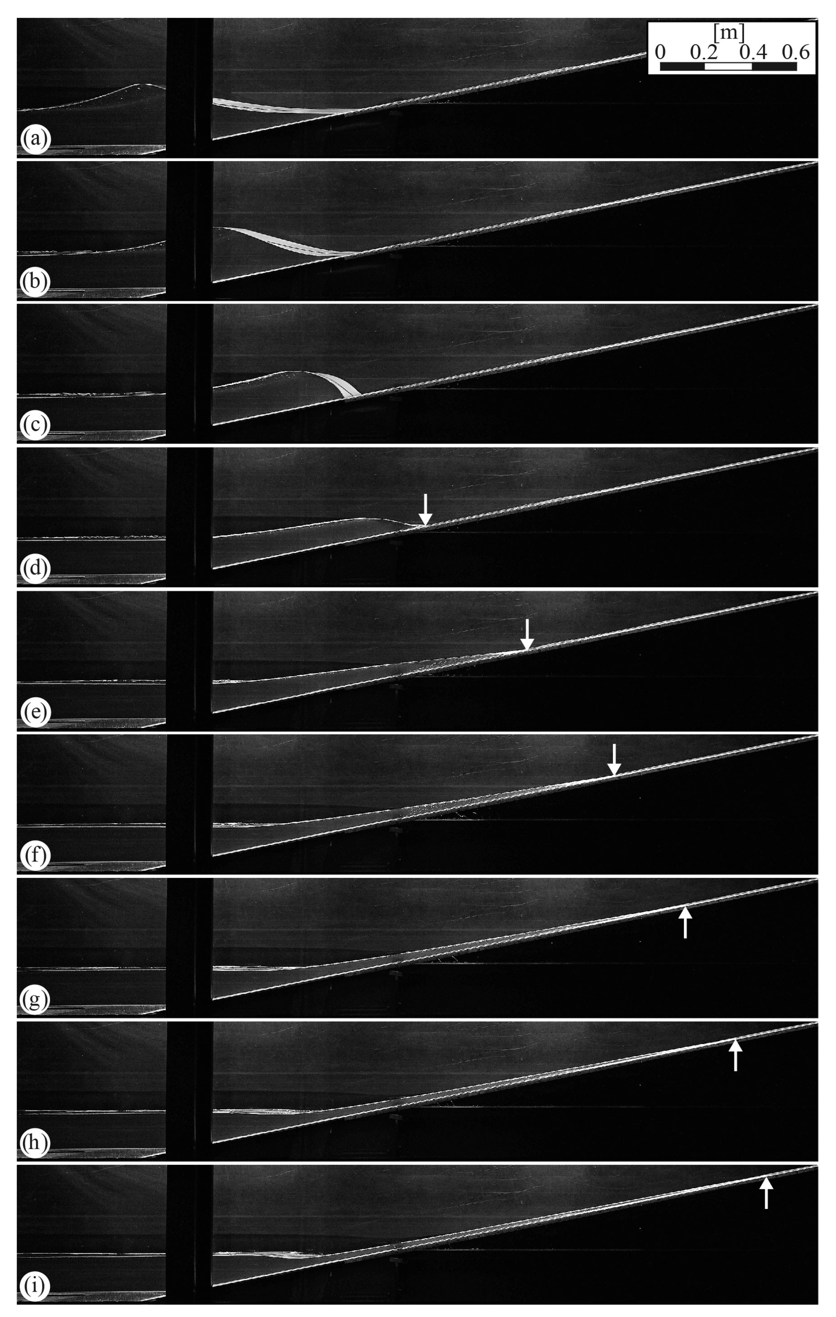
So ≥ 0.37. The experiment by Fuchs [
20] with
So = 0.37 (
Figure 3),
β ≈ 11.3°, and
ε = 0.69 is shown in
Figure 4 and features no distinct wave breaking characteristics. It is therefore assumed that the overall dataset consists of non-breaking wave runup. The limiting criterion
ε0.5 ≫ 0.288 tan
β for Equation (5) stated by Synolakis [
16] may be reformulated as
So ≪ 5.28 (Pujara et al. [
10]) and is also included in
Figure 3. Several experiments feature
So values close to and larger than 5.28.
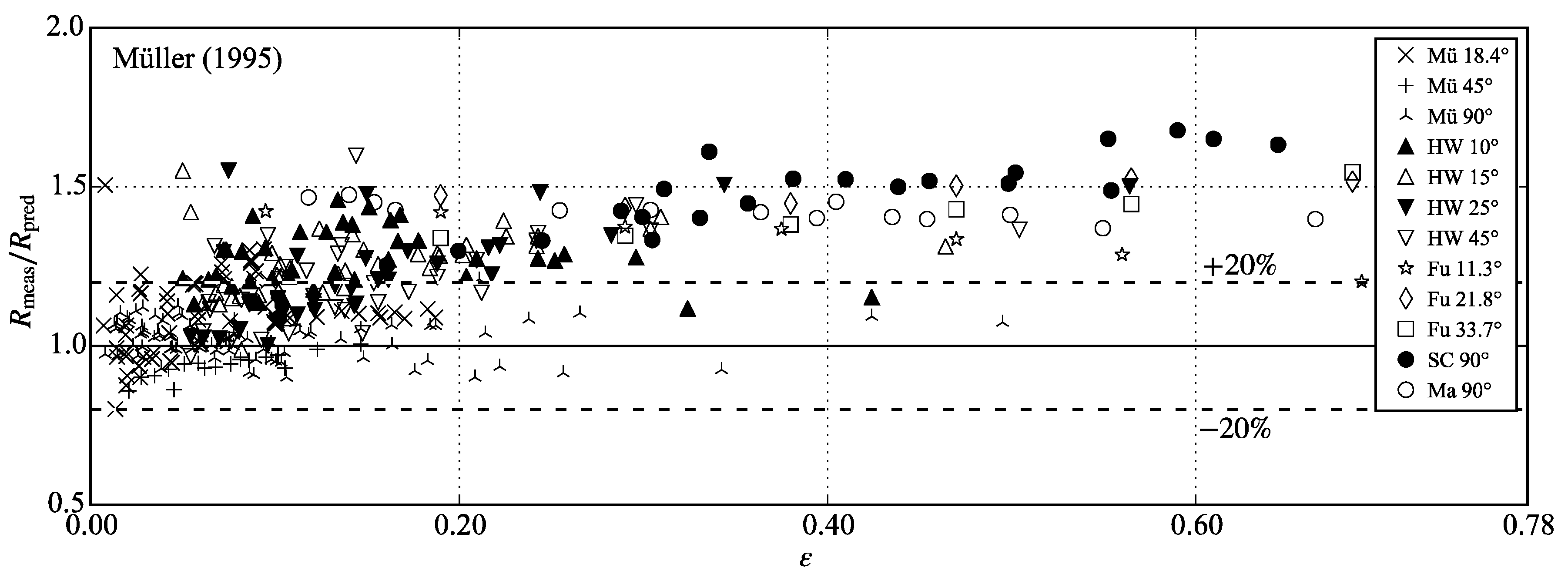
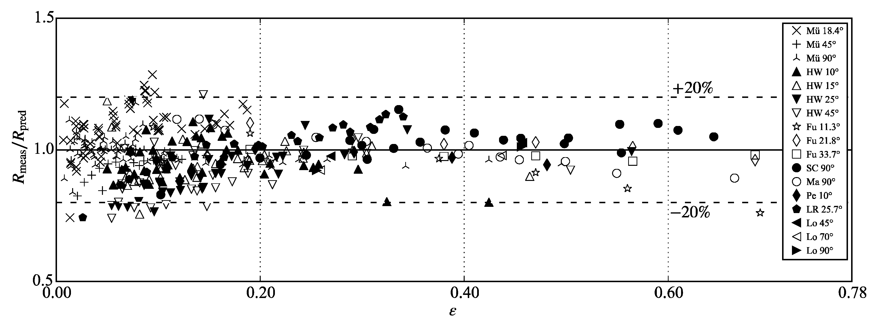
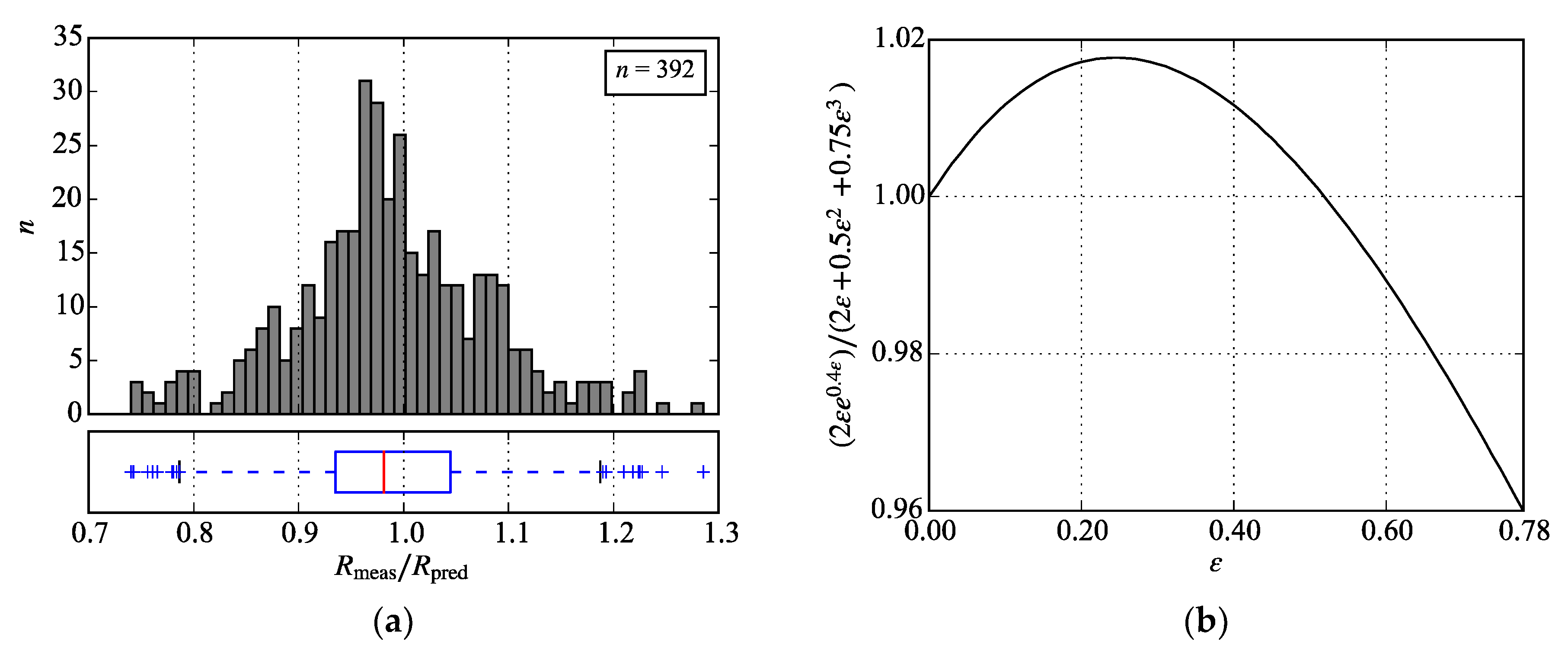
5. Discussion
With
So ≥ 0.37, the overall dataset is assumed to include non-breaking wave runup. Considering a maximum relative wave crest amplitude
ε = 0.78 before runup according to McCowan [
31], the minimum slope angle satisfying
So = 0.37 is
β = 12°. For this study, also experiments with
β = 10° and 11.3° were analyzed, which would lead to wave breaking for
ε = 0.78 according to
So. Equation (10) tends to overestimate runup heights by large
ε on these slopes (
Figure 12). Therefore
So = 0.37 is considered the lower application boundary of Equation (10) for
β from 10° to 90°. Pujara et al. [
10] proposed a more conservative breaking criterion
So ≈ 0.4 to 0.5. With
So > 0.5 to ensure no wave-breaking at
β = 10°, the maximum amplitude is
ε ≤ 0.3, which still provides a useful range of application for less steep slopes.
Compared to Equation (1) by Müller [
7], the new prediction Equation (10) contains solely the relative wave crest amplitude
ε as the governing wave parameter instead of the wave height
H and the wave length
L. For the assessment of landslide generated impulse wave events, prediction equations are applied in sequence to cover a particular process chain, e.g., wave generation and runup (Bregoli et al. [
8], McFall and Fritz [
9]). In this context, the maximum relative scatter of a target value, e.g.,
R, is derived from the scatter of its individual input parameters, e.g.,
ε,
H and/or
L (Heller et al. [
1]). While the scatter is not significantly altered by substituting
H and
L with
ε for predicting Müller’s [
7] measurements (
Figure 5 and
Figure 12), the prediction uncertainty for the entire process chain may be reduced by including fewer parameters.
Fuchs and Hager [
32] conducted scale family experiments of solitary wave runup and observed no significant scale effects for
h ≥ 0.08 m at
β = 11.3°. For their smallest investigated
ε = 0.1, this corresponds to a minimum runup height
R = 25 mm. The dataset by Müller [
7] contains six experiments at
β = 18.4° with
R between 12 and 24 mm induced by
ε from 0.007 to 0.014. As shown in
Figure 12, these experiments scatter around ±20% of the prediction. This range reflects the measurement accuracy as well as the experimental accuracy from repeatability tests (Müller [
7]). As no distinct trend is observed in the data, scale effects are considered negligible. Also, the experiments by Maxworthy [
19] feature
R < 25 mm. However, these experiments were conducted at a much steeper slope with
β = 90°. In addition, the measured runup heights show no distinct deviation compared to the experiments by Street and Camfield [
21], which were conducted at a three to four times larger scale (
Figure 9).
The experimental setups considered in this study feature two-dimensional, plane, and smooth runup slopes, which represent a simplification of shorelines at prototype scale. Additional prototype parameters include three-dimensional slope features, non-constant slopes, and rough surfaces. Strong curvatures along the shoreline cause flow diversion and concentration, respectively, which might lead to a significant over- or underestimation of the actual runup height. Therefore, Equation (10) should only be applied to evenly formed slope bathymetries and topographies. Non-constant slopes complicate the determination of a single slope angle
β. A sensitivity analysis allows for assessing the influence of
β for the slope range derived from field data. The term of Equation (10) including the slope angle
β yields larger runup heights for decreasing
β. A decrease from 90° to 45° leads to an increase in runup height of 15%. A decrease from 20° to 10° also leads to an increase of 15%. Therefore, the effect of
β is stronger for lower slope angles. Teng et al. [
33] conducted experiments on solitary wave runup on both smooth and rough slopes. The roughness effect was found to be negligible on relatively steep slopes (
β ≥ 20°), while it reduced the measured runup heights by up to approximately 30% for
β = 15° and by 50% for
β = 10°. However, runup height estimation based on Equation (10), which is derived from experiments featuring smooth slopes, would err on the side of caution. Finally, the scatter range of ±20% needs to be taken into account as a safety margin for runup height predictions at prototype scale.


