Water Quality Model Calibration via a Full-Factorial Analysis of Algal Growth Kinetic Parameters

Abstract
1. Introduction
2. Materials and Methods
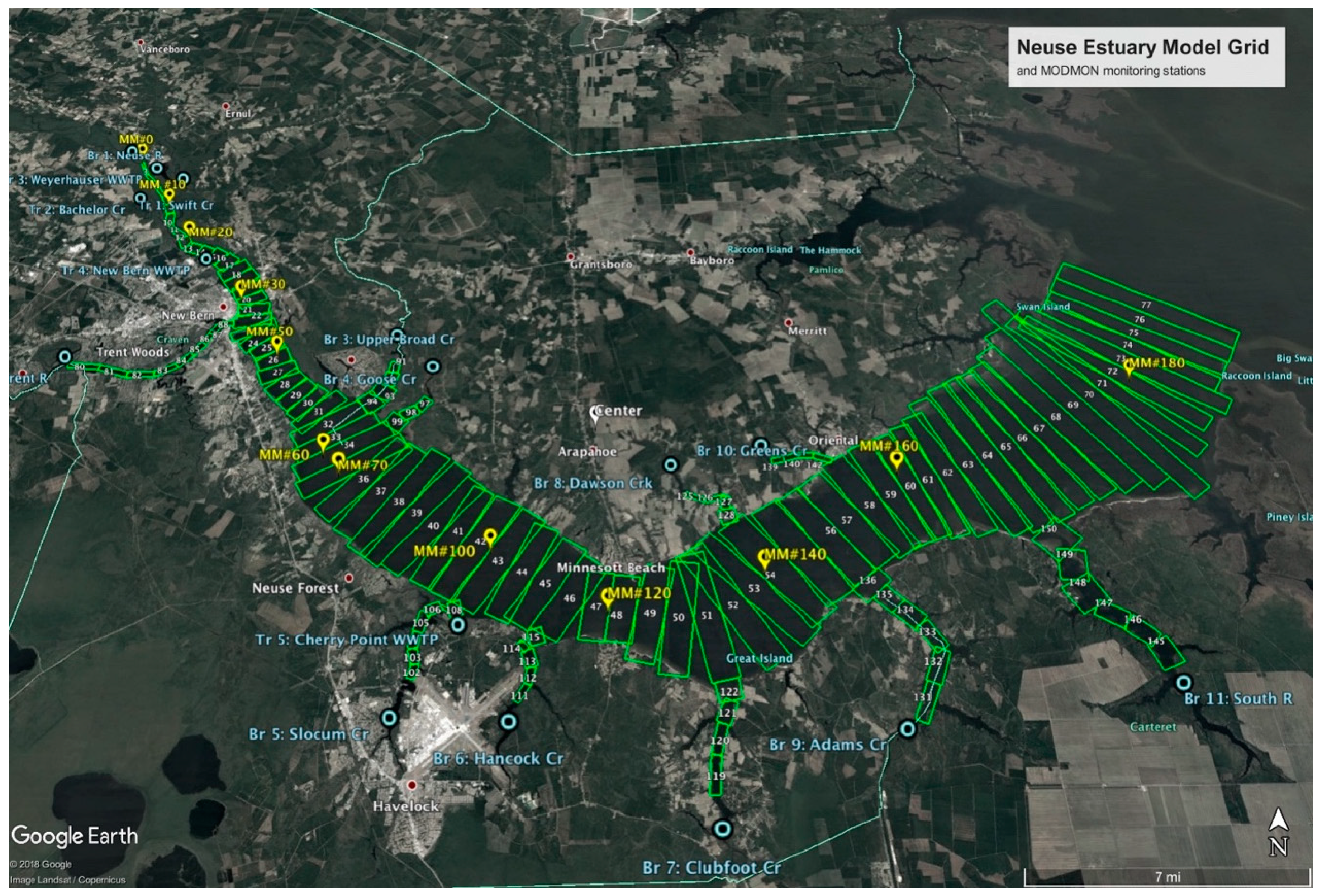
2.1. Model Set-Up
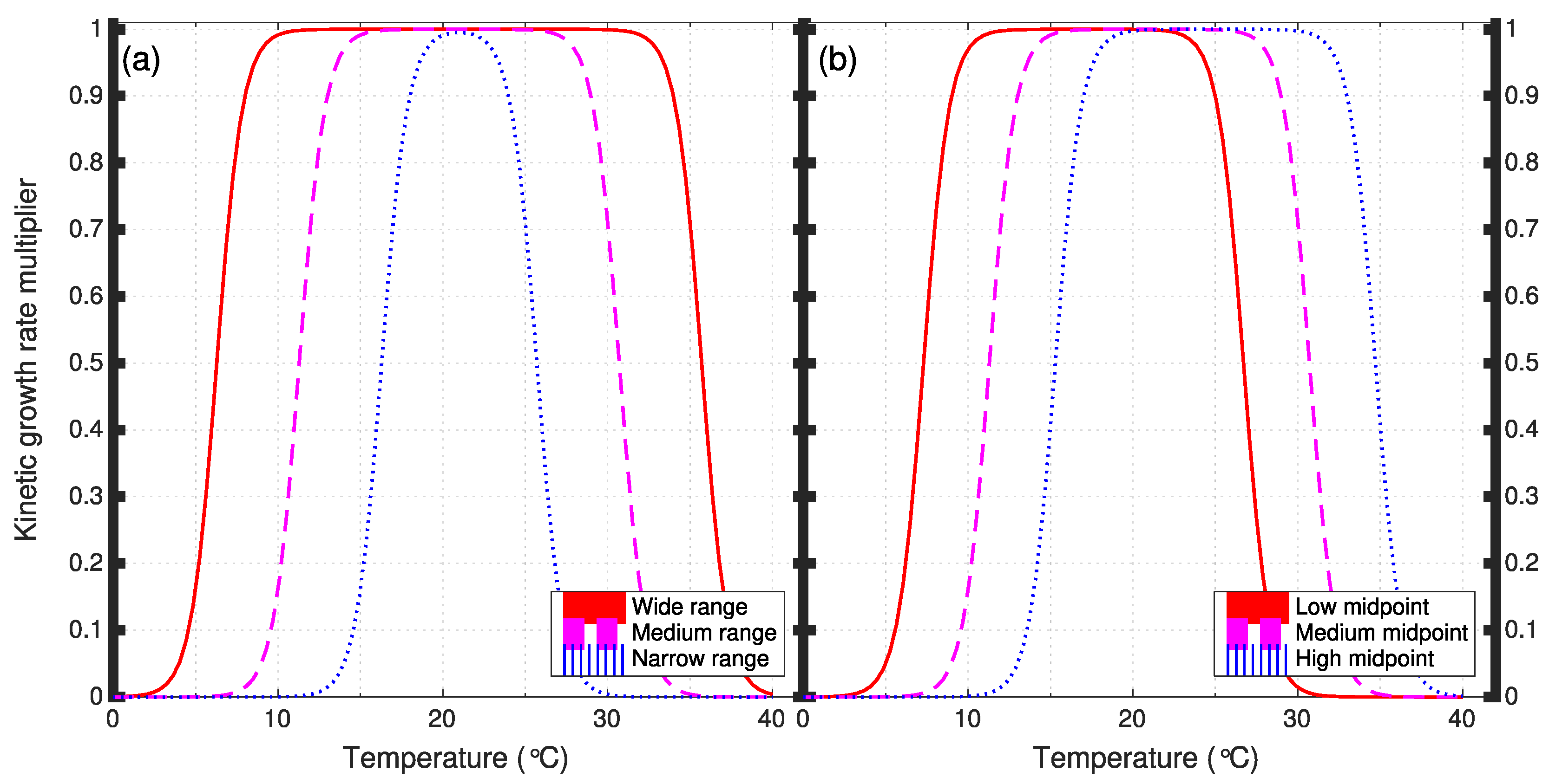
2.2. Algal Growth Parameters
2.3. Run Management
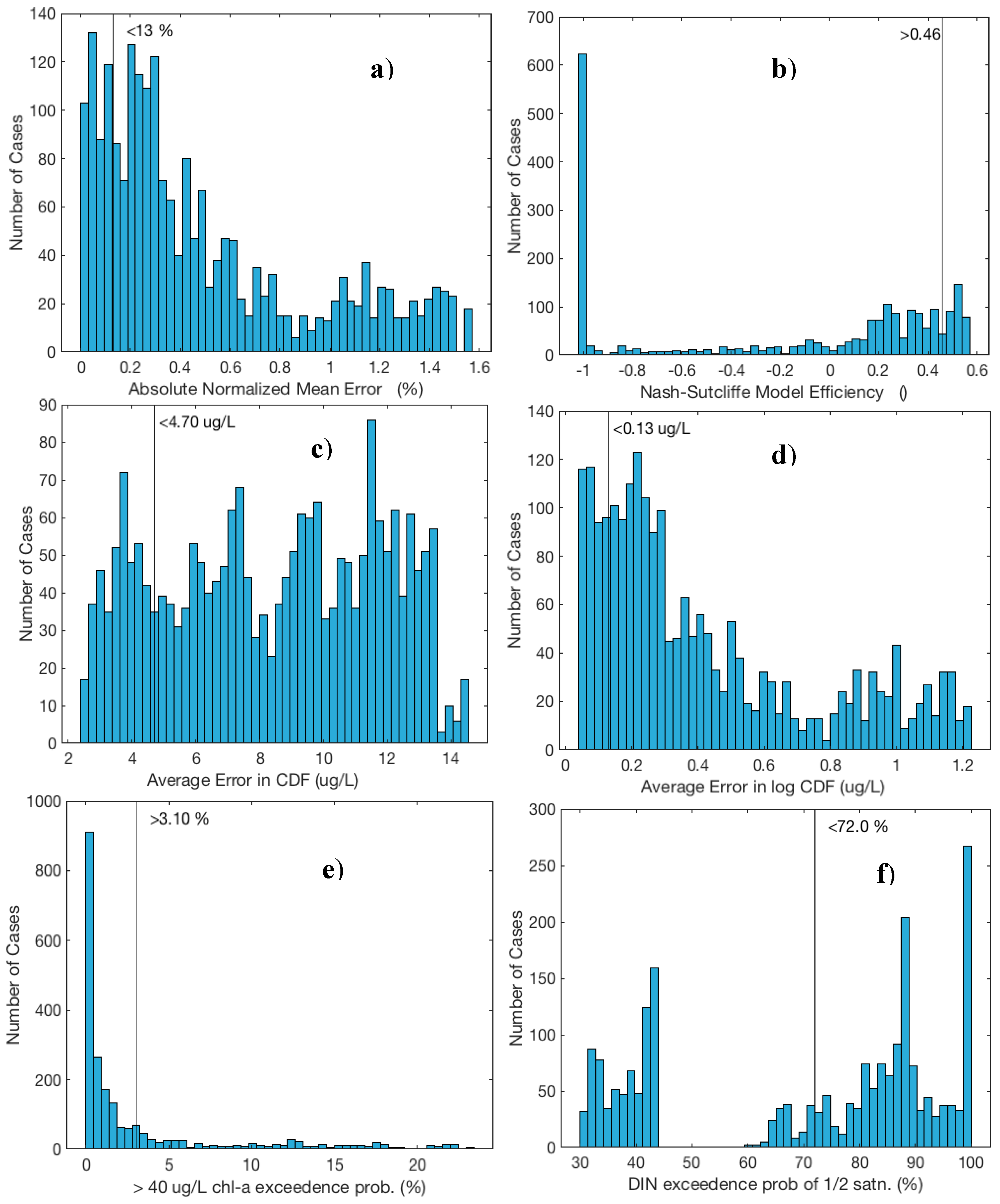
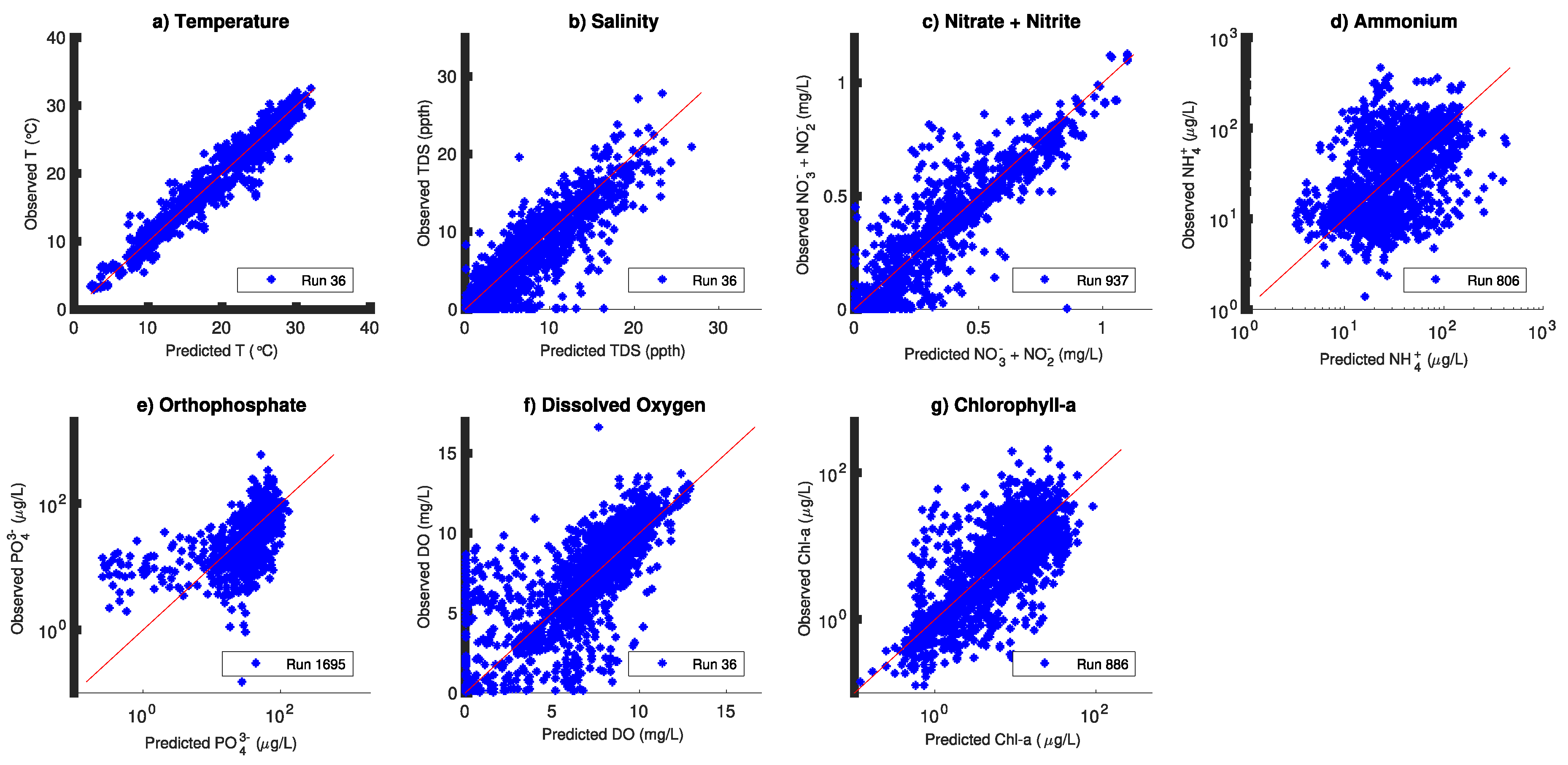
3. Results
4. Discussion
5. Summary
Author Contributions
Funding
Conflicts of Interest
References
- Paerl, H.W. Nuisance phytoplankton blooms in coastal, estuarine, and inland waters. Limnol. Oceanogr. 1988, 33, 823–847. [Google Scholar] [CrossRef]
- Pinckney, J.L.; Millie, D.F.; Vinyard, B.T.; Paerl, H. Environmental controls of phytoplankton bloom dynamics in the Neuse River Estuary, North Carolina, USA. Can. J. Fish. Aquat.Sci. 1997, 54, 2491–2501. [Google Scholar] [CrossRef]
- Stow, C.A.; Roessler, C.; Borsuk, M.E.; Bowen, J.D.; Reckhow, K.H. Comparison of estuarine water quality models for total maximum daily load development in Neuse River Estuary. J. Water Resour. Plan. Manag. 2003, 129, 307–314. [Google Scholar] [CrossRef]
- Bowen, J.D.; Hieronymus, J.W. A CE-QUAL-W2 model of Neuse Estuary for total maximum daily load development. J. Water Resour. Plan. Manag. 2003, 129, 283–294. [Google Scholar] [CrossRef]
- Bowen, J.D.; Hieronymus, J. Neuse River Estuary Modeling and Monitoring Project Stage 1: Predictions and Uncertainty Analysis of Response to Nutrient Loading Using a Mechanistic Eutrophication Model; Report No. 325 for Water Resources Research; Institute of the University of North Carolina: Raleigh, NC, USA, October 2000. [Google Scholar]
- Paerl, H.W.; Hall, N.S.; Peierls, B.L.; Rossignol, K.L.; Joyner, A.R. Hydrologic variability and its control of phytoplankton community structure and function in two shallow, coastal, lagoonal ecosystems: the Neuse and New River Estuaries, North Carolina, USA. Estuaries Coasts 2014, 37, 31–45. [Google Scholar] [CrossRef]
- Lebo, M.E.; Paerl, H.W.; Peierls, B.L. Evaluation of progress in achieving TMDL mandated nitrogen reductions in the Neuse River Basin, North Carolina. Environ. Manag. 2012, 49, 253–266. [Google Scholar] [CrossRef] [PubMed]
- Paerl, H.W.; Valdes, L.M.; Piehler, M.F.; Stow, C.A. Assessing the effects of nutrient management in an estuary experiencing climatic change: The Neuse River Estuary, North Carolina. Environ. Manag. 2006, 37, 422–436. [Google Scholar] [CrossRef] [PubMed]
- Hieronymus, J.; Bowen, J.D. Calibration and Verification of a Two-dimensional Laterally Averaged Mechanistic Model of the Neuse River Estuary; Report No. 343c for Water Resources Research; Institute of the University of North Carolina: Raleigh, NC, USA, July 2004. [Google Scholar]
- Liu, W.C.; Chen, W.B.; Kimura, N. Impact of phosphorus load reduction on water quality in a stratified reservoir-eutrophication modeling study. Environ. Monit. Assess. 2009, 159, 393–406. [Google Scholar] [CrossRef] [PubMed]
- Etemad-Shahidi, A.; Afshar, A.; Alikia, H.; Moshfeghi, H. Total dissolved solid modeling; Karkheh reservoir case example. Int. J. Environ. Res. 2009, 3, 671–680. [Google Scholar]
- Gelda, R.K.; Effler, S.W. Testing and application of a two-dimensional hydrothermal model for a water supply reservoir: Implications of sedimentation. J. Environ. Eng. Sci. 2007, 6, 73–84. [Google Scholar] [CrossRef]
- Huang, Y.; Liu, L. Multiobjective water quality model calibration using a hybrid genetic algorithm and neural network–based approach. J. Environ. Eng. 2010, 136, 1020–1031. [Google Scholar] [CrossRef]
- Afshar, A.; Kazemi, H.; Saadatpour, M. Particle swarm optimization for automatic calibration of large scale water quality model (CE-QUAL-W2): Application to Karkheh Reservoir, Iran. Water Resour. Manag. 2011, 25, 2613–2632. [Google Scholar] [CrossRef]
- Afshar, A.; Shojaei, N.; Sagharjooghifarahani, M. Multiobjective calibration of reservoir water quality modeling using multiobjective particle swarm optimization (MOPSO). Water Resour. Manag. 2013, 27, 1931–1947. [Google Scholar] [CrossRef]
- Grangere, K.; Lefebvre, S.; Ménesguen, A.; Jouenne, F. On the interest of using field primary production data to calibrate phytoplankton rate processes in ecosystem models. Estuar. Coast. Shelf Sci. 2009, 81, 169–178. [Google Scholar] [CrossRef]
- Arhonditsis, G.B.; Papantou, D.; Zhang, W.T.; Perhar, G.; Massos, E.; Shi, M. Bayesian calibration of mechanistic aquatic biogeochemical models and benefits for environmental management. J. Mar. Syst. 2008, 73, 8–30. [Google Scholar] [CrossRef]
- Arhonditsis, G.B.; Qian, S.S.; Stow, C.A.; Lamon, E.C.; Reckhow, K.H. Eutrophication risk assessment using Bayesian calibration of process-based models: Application to a mesotrophic lake. Ecol. Model. 2007, 208, 215–229. [Google Scholar] [CrossRef]
- Bowen, J.; Harrigan, N.B. Comparing the Impact of Organic Versus Inorganic Nitrogen Loading to the Neuse River Estuary With a Mechanistic Eutrophication Model; Report No. 470 for Water Resources Research; Institute of the University of North Carolina: Raleigh, NC, USA, September 2017. [Google Scholar]
- Cole, T.M.; Wells, S.A. CE-QUAL-W2: A Two-Dimensional, Laterally Averaged, Hydrodynamic and Water Quality Model, Version 3.72 User Manual; Technical Report; Department of Civil and Environmental Engineering, Portland State University: Portland, OR, USA, 2015. [Google Scholar]
- Paerl, H.W.; Rossignol, K.L.; Hall, S.N.; Peierls, B.L.; Wetz, M.S. Phytoplankton community indicators of short-and long-term ecological change in the anthropogenically and climatically impacted Neuse River Estuary, North Carolina, USA. Estuaries Coasts 2010, 33, 485–497. [Google Scholar] [CrossRef]
- Paerl, H.W.; Valdes, L.M.; Peierls, B.L.; Adolf, J.E.; Harding, L.J.W. Anthropogenic and climatic influences on the eutrophication of large estuarine ecosystems. Limnol. Oceanogr. 2006, 51, 448–462. [Google Scholar] [CrossRef]
- Steele, J.H. Environmental control of photosynthesis in the sea. Limnol. Oceanogr. 1962, 7, 137–150. [Google Scholar] [CrossRef]
- Thornton, K.W.; Lessem, A.S. A temperature algorithm for modifying biological rates. Trans. Am. Fish. Soc. 1978, 107, 284–287. [Google Scholar] [CrossRef]
- McCuen, R.H.; Knight, Z.; Cutter, A.G. Evaluation of the Nash–Sutcliffe efficiency index. J. Hydrol. Eng. 2006, 11, 597–602. [Google Scholar] [CrossRef]
- Krause, P.; Boyle, D.; Bäse, F. Comparison of different efficiency criteria for hydrological model assessment. Adv. Geosci. 2005, 5, 89–97. [Google Scholar] [CrossRef]
- Boyer, J.N.; Christian, R.R.; Stanley, D.W. Patterns of phytoplankton primary productivity in the Neuse River estuary, North Carolina, USA. Mar. Ecol. Prog. Ser. 1993, 97, 287–297. [Google Scholar] [CrossRef]
- Wool, T.A.; Davie, S.R.; Rodriguez, H.N. Development of three-dimensional hydrodynamic and water quality models to support total maximum daily load decision process for the Neuse River Estuary, North Carolina. J. Water Resour. Plan. Manag. 2003, 129, 295–306. [Google Scholar] [CrossRef]


| No. | Constituent | Unit |
|---|---|---|
| 1 | Salinity (TDS) | g/L |
| 2 | Tracer | mg/L |
| 3 | Inorganic Suspended Solids (ISS) = Salinity (TDS) | mg/L |
| 4 | Orthophosphate (PO43-) | mg/L |
| 5 | Ammonium (NH4+) | mg/L |
| 6 | Nitrate-Nitrite (NO3- + NO2-) | mg/L |
| 7 | Dissolved Silica | mg/L |
| 8 | Labile Dissolved Organic Matter (L-DOM) | mg/L |
| 9 | Refractory Dissolved Organic Matter (R-DOM) | mg/L |
| 10 | Labile Particulate Organic Matter (L-POM) | mg/L |
| 11 | Refractory Particulate Organic Matter (R-POM) | mg/L |
| 12 | Biological Oxygen Demand (BOD) | mg/L |
| 13 | Algal Group | mg/L |
| 14 | Dissolved Oxygen | mg/L |
| Parameter | W2 Designation | Unit | Low Value | Middle Value | High Value |
|---|---|---|---|---|---|
| Maximum algal growth rate | AG | d−1 | 0.553 | 1.75 | 5.53 |
| Maximum algal respiration rate | AR | d−1 | 0.0116 | 0.0367 | 0.116 |
| Maximum algal excretion rate | AE | d−1 | 0.00949 | 0.0300 | 0.0949 |
| Maximum algal mortality rate | AM | d−1 | 0.00528 | 0.0167 | 0.0528 |
| Algal settling rate | AS | m d−1 | 0.0136 | 0.0430 | 0.136 |
| Algal half-saturation for phosphorus-limited growth | AHSP | g m−3 | 0.00219 | 0.00693 | 0.0219 |
| Algal half-saturation for nitrogen-limited growth | AHSN | g m−3 | 0.0164 | 0.0520 | 0.164 |
| Algal half-saturation for silica-limited growth | AHSSI | g m∑3 | 0.0001 | 0.0001 | 0.0001 |
| Light saturation intensity at maximum photosynthetic rate | ASAT | W m∑2 | 39.53 | 125.0 | 395.3 |
| Width of rate-multiplier function | AT4−AT1 | °C | 14 | 24 | 34 |
| Midpoint of rate-multiplier function | (AT1+AT4)/2 | °C | 17 | 21 | 25 |
| Criteria | Constituent | Variable | Condition | # Meeting Criteria (Out of 2187 Trials) |
|---|---|---|---|---|
| 1 | CHLA | Abs normalized mean error | <13% | 450 |
| 2 | CHLA | Nash–Sutcliffe model efficiency | >46% | 339 |
| 3 | CHLA | 40 µg/L exceedance probability | >3.1% | 542 |
| 4 | CHLA | Average CDF error | <4.70 µg/L | 417 |
| 5 | CHLA | Average log CDF error | <0.13 µg/L | 406 |
| 6 | DIN | ½ saturation exceedance probability | <72% | 894 |
| # Meeting ALL criteria = | 27/2187 = 1.2% | |||
| Constituent | ME (%) | MAE (%) | RMSE (%) | Nash–Sutcliffe Model Efficiency (%) | # obs. |
|---|---|---|---|---|---|
| Temperature | 0.71 ± 0 (0%) | 5.59 ± 0 (0%) | 7.58 ± 0 (0%) | 96.0 ± 0 (0%) | 3252 |
| Salinity | 10.4 ± 0 (0%) | 249 ± 0 (0%) | 37.1 ± 0 (0%) | 85.1 ± 0 (0%) | 3252 |
| Ext. coefficient | 1.29 ± 0 (0%) | 20.8 ± 0 (0%) | 27.1 ± 0 (0%) | 46.2 ± 0 (0%) | 1540 |
| Nitrate | 1.90 ± 0.1 (27%) | 224 ± 1 (1%) | 33.7 ± 0.4 (1%) | 83.0 ± 0.4 (0.4%) | 1956 |
| Ammonia | ∑15.3 ± 2.8 (19%) | 66.0 ± 1 (2%) | 127 ± 0.9 (0.7%) | ∑13.1 ± 1.6 (12%) | 3175 |
| Phosphate | 0.92 ± 2 (220%) | 55.0 ± 2.4 (4.4%) | 100 ± 4.0 (4%) | 12.4 ± 6.8 (55%) | 3005 |
| Dissolved O2 | ∑5.50 ± 0.60 (11%) | 20.4 ± 0.03 (0.14%) | 29.7 ± 0.07 (0.25%) | 51.1 ± 0.20 (0.5%) | 3252 |
| Chlorophyll-a | 11.6 ± 0.80 (7%) | 35.8 ± 0.60 (1.7%) | 47.4 ± 0.80 (1.6%) | 49.3 ± 1.6 (3.2%) | 3182 |
© 2018 by the authors. Licensee MDPI, Basel, Switzerland. This article is an open access article distributed under the terms and conditions of the Creative Commons Attribution (CC BY) license (http://creativecommons.org/licenses/by/4.0/).
Share and Cite
Bowen, J.D.; Harrigan, N.B. Water Quality Model Calibration via a Full-Factorial Analysis of Algal Growth Kinetic Parameters. J. Mar. Sci. Eng. 2018, 6, 137. https://doi.org/10.3390/jmse6040137
Bowen JD, Harrigan NB. Water Quality Model Calibration via a Full-Factorial Analysis of Algal Growth Kinetic Parameters. Journal of Marine Science and Engineering. 2018; 6(4):137. https://doi.org/10.3390/jmse6040137
Chicago/Turabian StyleBowen, James D., and Noyes B. Harrigan. 2018. "Water Quality Model Calibration via a Full-Factorial Analysis of Algal Growth Kinetic Parameters" Journal of Marine Science and Engineering 6, no. 4: 137. https://doi.org/10.3390/jmse6040137
APA StyleBowen, J. D., & Harrigan, N. B. (2018). Water Quality Model Calibration via a Full-Factorial Analysis of Algal Growth Kinetic Parameters. Journal of Marine Science and Engineering, 6(4), 137. https://doi.org/10.3390/jmse6040137