Assessment of Scale Effects, Viscous Forces and Induced Drag on a Point-Absorbing Wave Energy Converter by CFD Simulations

Abstract

This paper analyses the nonlinear forces on a moored point-absorbing wave energy converter (WEC) in resonance at prototype scale (1:1) and at model scale (1:16). Three simulation types were used: Reynolds Averaged Navier–Stokes (RANS), Euler and the linear radiation-diffraction method (linear). Results show that when the wave steepness is doubled, the response reduction is: (i) 3% due to the nonlinear mooring response and the Froude–Krylov force; (ii) 1–4% due to viscous forces; and (iii) 18–19% due to induced drag and non-linear added mass and radiation forces. The effect of the induced drag is shown to be largely scale-independent. It is caused by local pressure variations due to vortex generation below the body, which reduce the total pressure force on the hull. Euler simulations are shown to be scale-independent and the scale effects of the WEC are limited by the purely viscous contribution (1–4%) for the two waves studied. We recommend that experimental model scale test campaigns of WECs should be accompanied by RANS simulations, and the analysis complemented by scale-independent Euler simulations to quantify the scale-dependent part of the nonlinear effects.

1. Introduction

The performance of wave energy concept designs is evaluated by the combined effort of physical experiments and numerical tools. The most common road-map from early stage development towards commercialization is to use experimental model tests as a proof-of-concept, typically followed by the calibration and validation of a numerical model of wave-to-wire type to estimate the power production of the design [1]. To advance further in technical readiness level (TRL) [2], a larger device needs to be designed for sea-trials. However, the combined experience and know-how of wave power installations in larger scales is still limited, and the up-scaling to field testing dimensions is not only associated with large capital investments but also with significant uncertainties in the design method.

Numerical models based on the radiation-diffraction approach are still widely used in the wave energy community, although computational fluid dynamics (CFD) modelling has recently come into focus. Using fully nonlinear Reynolds Averaged Navier–Stokes (RANS) simulations with the volume of fluid (VOF) method for the air-water interface has emerged as the most common method of choice in CFD for wave energy applications [3]. Many studies of point-absorbing WECs (PAWECs) have been presented over the last few years, e.g., [4,5,6,7,8,9,10], which has already spurred some reviews of the nonlinear numerical approaches to WEC design [3,11,12,13].

The two main nonlinearities affecting PAWECs in the resonance region are drag forces and nonlinear Froude–Krylov (FK) forcing. The nonlinear FK force can be well accounted for in quasi-linear radiation-diffraction (wave-to-wire) codes as it is a purely geometric effect [14]. Drag forces are also commonly included in parametrised form as in the Morison equation [15], but this requires calibration of drag coefficients. Such calibration is then made via experiments (see e.g., Rodriguez and Spinnekens work on a heaving box [16,17]) or via CFD simulations (as in the viscous correction method of Bhinder et al. [18]). The work of Stansby et al. [19] and Gu et al. [20] present RANS simulations of different cylinder bottom geometries in surge and heave decay. The inferred drag coefficients point to that the surge drag was much higher than the heave drag, and that the heave drag influence increases as the bottom shape changes from hemisphere, to rounded corners with flat centres to a truncated cylinder. Although significant drag force was obtained, the shear forces were very small overall. Also Chen et al. [7] conclude from heave decay tests that the viscous effects are the largest for a flat bottom. They also highlight the difference in flow pattern surrounding the WEC for the different body shapes and put forward viscous correction factors, which are deduced from the deviation of the WEC decay motion from potential theory. In a recent series of papers Giorgi and co-authors [14,21,22] discuss a case study of a spherical floater in heave. They show that weakly non-linear potential flow simulations with calibrated parametrised drag force give results much closer to CFD prediction than simulations using only nonlinear FK corrections. Further analysis about the individual force contributions shows how the viscous contribution is particularly important under latching control conditions were the relative velocities increase. The same conclusion regarding relative velocity and drag force is reported also by Jin and Patton [23], based on a CFD and experimental study of a heaving cylinder.

Viscous effects are dominated by the Reynolds number, which does not scale with Froude scaling laws [24]. However, other drag types such as the form drag (e.g., around bilge keels on ships) and the induced drag (from geometrically induced vortices) are independent of scale. So a consistent treatment of drag for WECs at different scales should include a separation of the total drag into a scale-independent drag component, and a viscous drag term [24,25,26]. This is not only a semantic issue. When the drag force is computed from the difference between potential flow and incompressible VOF-RANS simulations it is the total drag force which is produced, and its relevance to wave-to-wire model calibration is tied to the scale at which it was made. A method to separate the drag force into Reynolds dominated and Froude dominated effects would be very beneficial in this context.

There is a direct link between scale effects and drag forces of offshore structures. Effects of scale are well understood for traditional marine structures, referring here to Sarpkaya and Isacson [27] who present an extensive compilation of research on the drag force contribution in oscillating flow. Relations between the nondimensional Keulegan–Carpenter number and the Reynolds number dictate the contribution of inertial forces versus drag forces at different scales. Studies of scaling effects on WECs are however very few. An investigation of oscillating wave surge (OWS) WECs was presented by Wei et al. [26] and includes a thorough CFD analysis of differences between the scales for the pitch motion of the flap-type device. They conclude that scale effects (down to 1:100) are observed but that the overall response is scale independent, and that the use of a calibrated Morison-type drag correction is not suitable for OWS WECs. Schmitt & Elsaesser [28] then varied the viscosity in model scale to achieve perfect similitude in both Froude and Reynolds scales, which lead to 2–3% larger integral forces compared with the model scale with physical water properties. Also, Pathak et al. [29] show small effects of scale on a OWS device. The line point-absorber M4 was investigated experimentally by Stansby et al. [30] at scales (1:8) and (1:40), showing differences in capture width ratio for flat-bottomed floats. Experiments were made in two different wave tanks so the results are not completely conclusive, however, they still represent an important contribution to the methodology of WEC design. The heave drag coefficients were numerically obtained for the floats by RANS CFD at both scales showing a small but notable decrease of the coefficient as the physical size increased, as well as an increase in coefficient as the amplitude of the decay motion increased [20].

This paper analyses two important and inter-connected problems: (i) the scale effects between a model scale and a prototype-scale (full-scale) device, which boils down to quantifying the Reynolds dominated effects of viscosity at the two scales; and (ii) the drag damping responsible for a severe reduction in RAO at resonance when the wave steepness increases. The WEC is studied both as a fixed structure and as a moored WEC with power take off (PTO) for two regular wave cases in the heave resonance region. Scale effects on a cylindrical WEC are evaluated by comparing results from the full scale prototype (100 tonne mass, 5 m diameter) with a 1:16 scaled model. Inviscid Euler simulations are compared with RANS results to quantify the viscous contribution to the loads and responses of the WEC, and weakly non-linear radiation-diffraction theory is used as a reference for the prototype scale responses without any drag influence.

The paper is organized as follows. Section 2 lists the set-up of the moored generic WEC used in the study including the scaling between model and prototype scale. Section 3 summarizes the computational methods used in the paper, while Section 4 outlines how the results are presented. Section 5.1 presents the prototype scale simulations of the different computational methods. 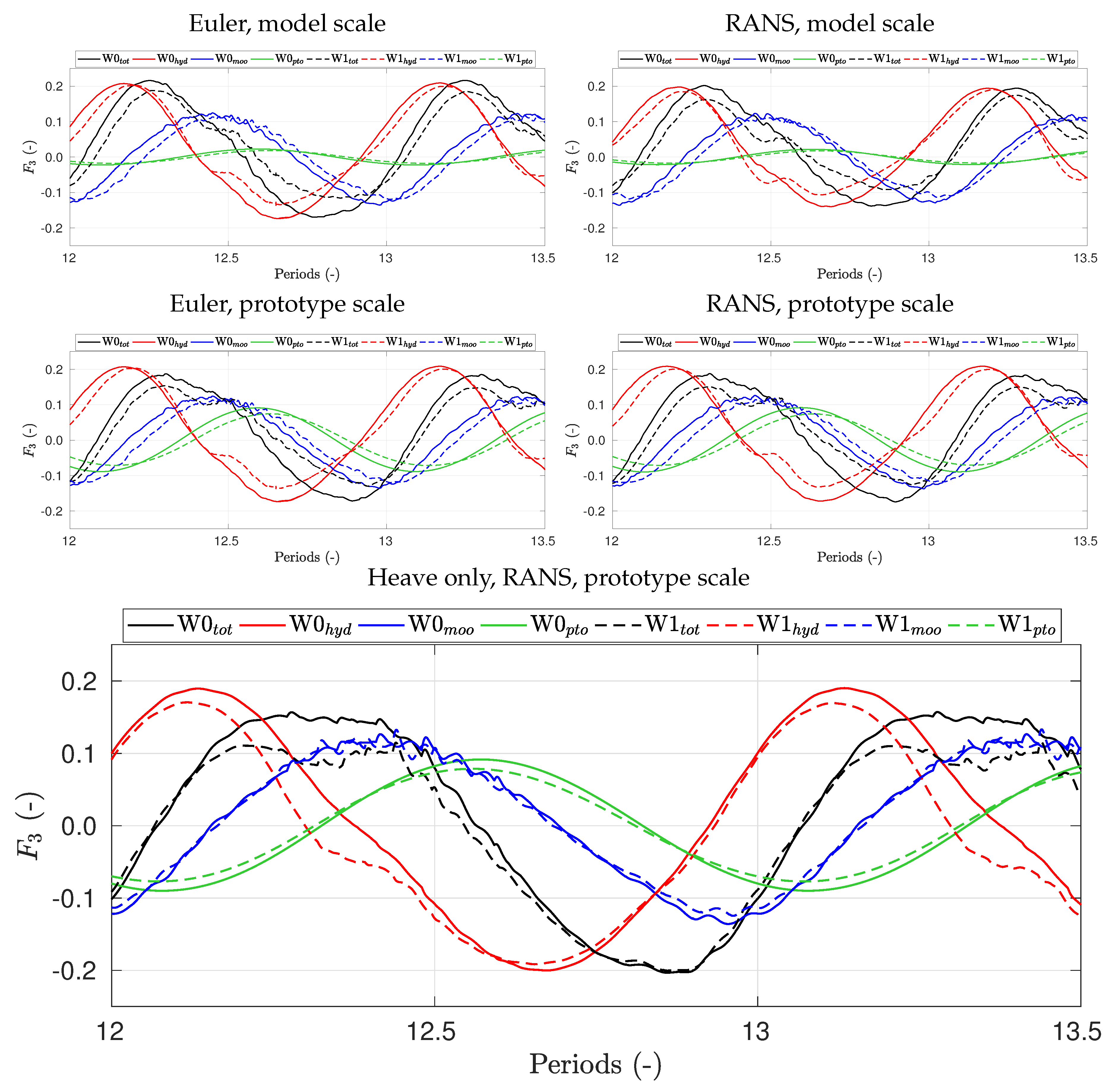These results are then compared with the model scale results in Section 5.2, followed by a detailed analysis of the heave response in Section 5.3. The heave analysis includes a force decomposition and visualisation of local flow structures and pressure distributions. The paper ends with a discussion in Section 6 and a conclusion in Section 7.

2. WEC Description

This paper uses the moored, generic buoy designed by Fitzgerald & Bergdahl [31] as a baseline prototype scale WEC. In addition, we study the same buoy as a 1:16 Froude scale model with scaled WEC, moorings, waves and wave tank dimensions. In the paper the subscripts p and m denote prototype and model scale, respectively. The (1:1) and (1:16) notation is also used when suitable. The prototype device is a vertical cylinder of 5 m diameter and 5 m draft in the unmoored equilibrium position. 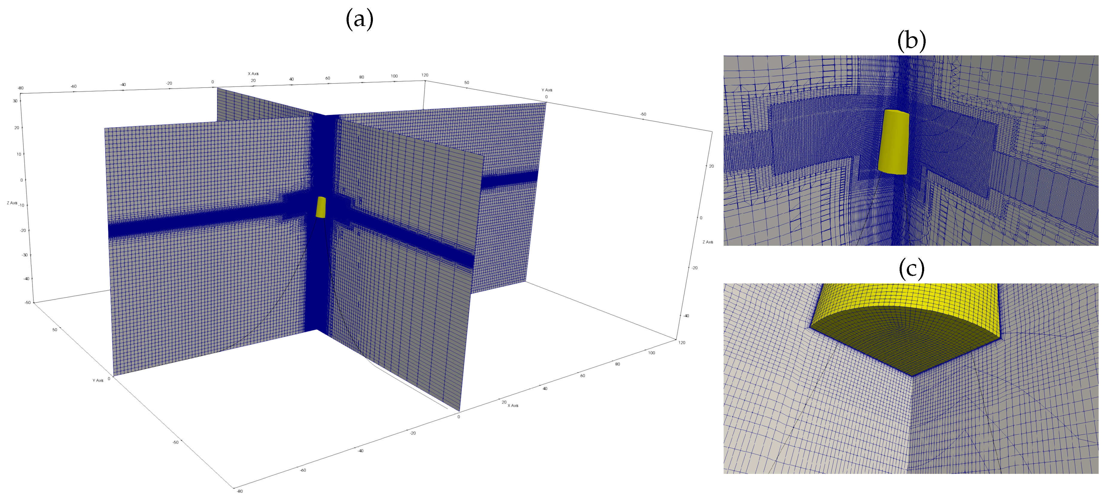The WEC is initially placed at $(x,y)=(0,0)$ m in a numerical wave tank (NWT) of 50 m water depth in prototype scale. It is moored with four steel chains that are axi-symmetrically attached to the bottom plate of the cylinder, as shown in Figure 1. The mooring chains are initially aligned with the horizontal coordinate axes (x and y) of the tank. The properties of the WEC itself and the mooring chains are for both scales detailed in

Table 1. Description of the WEC properties in prototype and model scales including scaling factors. Please note that the center of gravity refers to a position relative to an equilibrium still water level in unmoored conditions.

Property	Scaling	Value (1:1)	Value (1:16)
Water density, ${\rho }_w$ (kg/m${}^3$)	1	1025	1025
Diameter, D (m)	${\lambda }^{*}$	5	3.125 × 10${}^{-1}$
Draft, unmoored (m)	${\lambda }^{*}$	5	3.125 × 10${}^{-1}$
Draft, moored (m)	${\lambda }^{*}$	5.63	3.519 × 10${}^{-1}$
Center of gravity (m)	${\lambda }^{*}$	(0, 0, −2.418)	(0, 0, −1.511) × 10${}^{-1}$
Pitch and roll inertia (kgm${}^2$)	${{\lambda }^{*}}^5$	1.244 × 10${}^6$	1.186
Yaw inertia (kgm${}^2$)	${{\lambda }^{*}}^5$	4.717 × 10${}^5$	4.498 × 10${}^{-1}$
PTO damping coefficient, $b_{33}$ (Ns/m)	${{\lambda }^{*}}^{5/2}$	1.5 × 10${}^4$	1.465 × 10${}^1$

and

Table 2. Description of the mooring cable properties in prototype scale. Please note that the values of anchor and fairlead positions apply to the seaward cable, facing the wave direction. The other three mooring cables are found from rotation about the vertical axis with 90, 180, and 270 degrees respectively.

Property	Scaling	Value (1:1)	Value (1:16)
Cable density, ${\rho }_c$ (kg/m${}^3$)	1	7.8× 10${}^3$	7.8 × 10${}^3$
Mass per meter, ${\gamma }_0$ (kg/m)	${{\lambda }^{*}}^2$	6.1 × 10${}^1$	2.383 × 10${}^{-1}$
Length, L (m)	${\lambda }^{*}$	1 × 10${}^2$	6.25
Diameter, d (m)	${\lambda }^{*}$	5 × 10${}^{-2}$	3.125 × 10${}^{-3}$
Axial stiffness, $EA$ (N)	${{\lambda }^{*}}^3$	1 × 10${}^8$	2.441 × 10${}^4$
Added mass coefficient, $C_M$ (-)	1	3.8	3.8
Normal drag coefficient, $C_{DN}$ (-)	1	2.5	2.5
Tangential drag coefficient, $C_{DT}$ (-)	1	0.5	0.5
Seaward anchor point, $P_{\mathrm{A}}$ (m)	${\lambda }^{*}$	(−76.663, 0, −50)	(−4.791, 0, −3.125)
Seaward fairlead, $P_{\mathrm{B}}$ (m)	${\lambda }^{*}$	(−1.863, 0, −5)	(−1.164, 0, −3.125) × 10${}^{-1}$
Seabed stiffness (Pa/m)	1	1 × 10${}^6$	1 × 10${}^6$
Seabed damping ratio (-)	1	1.0	1.0
Seabed friction coefficient (-)	1	1	1
Seabed friction speed, $v_c$ (m/s)	${{\lambda }^{*}}^{1/2}$	0.1	2.5 × 10${}^{-2}$

, respectively. The fair-lead positions are in this study moved closer to the symmetry-axis of the cylinder compared with the original design [31]. Further, the PTO of the device has been changed to operate only in heave. It is implemented as a linear dash-pot directed along the instantaneous symmetry-axis of the cylinder, thus only acting on the body-local heave velocity.

Froude Scaling

We apply Froude scaling to achieve dynamic similitude between simulations at different scales. Froude scaling accounts for all potential flow parameters as well as separation due to large pressure gradients in the simulation, but it does not compensate for the viscous contribution of the shear stress. That depends on the Reynolds number. Hence, we expect the differences between Euler and RANS simulations to increase as we go from prototype to model scale size where the viscous effects are expected to be larger.

The length scale factor from prototype to model was ${\lambda }^{*}=1/16$. In simulations with waves, dynamic similitude of the wave form is only achieved when the time scale $t^{*}$ is set to $t^{*}=\sqrt{{\lambda }^{*}}$, based on the first order dispersion relation in deep water. For the moorings to have dynamic similitude, they are scaled according to the description in Bergdahl et al. [32]. Table 1 and Table 2 present the properties of the scaling used in this study. The parameters of drag and added mass for the mooring cables were kept constant across the scales, although the drag force would be scale-dependent in physical tests because of the difference in Reynolds number. Please note that the mooring drag forces are parametrised and modelled independently of the viscosity of the fluid in the CFD simulations, and that the moorings are simulated in still water conditions. Hence, the drag damping of the moorings is consistently modelled in all simulations and we therefore consider all differences between Euler and RANS results in the same scale to be attributed to differences in flow characteristics and in wave–body interactions.

3. Numerical Method

The WEC is modelled with the volume of fluid method on the Reynolds averaged Navier–Stokes equations (VOF-RANS). For this we use the OpenFOAM platform for finite volume simulations [33,34], via the interDyMFoam solver with its Arbitrary Lagrangian-Eularian (ALE) formulation. We use the waves2Foam library for wave generation and absorption [35], and coupled simulations with Moody [36,37] for dynamic mooring response. The dynamic mooring coupling to OpenFOAM and the methodology of the numerical setup was validated in model scale in [6].

3.1. VOF-RANS Equations

The incompressible RANS equations for a single fluid in an ALE formulation read:

$$\nabla ·{\mathbf{u}}_{\mathrm{r}}=0$$

(1)

$$\frac{\partial }{\partial t}(\rho \mathbf{u})+\nabla ·(\rho \mathbf{u}{\mathbf{u}}_{\mathrm{r}})=-\nabla p+\nabla ·\mathbf{S}+\rho {\mathbf{f}}_{\mathbf{b}}$$

(2)

where $\mathbf{u}$ is the fluid velocity. Further ${\mathbf{u}}_{\mathrm{r}}=\mathbf{u}-{\mathbf{u}}_{\mathrm{g}}$ is the relative velocity with respect to the grid velocity ${\mathbf{u}}_{\mathrm{g}}$. p is the total pressure, $\rho$ is the mixture density, $\mathbf{S}$ is the viscous stress tensor and ${\mathbf{f}}_{\mathbf{b}}$ is the volume force from buoyancy. OpenFOAM solves the RANS equations with a cell-centred method on unstructured polyhedral cells [34].

The VOF method solves the two-phase problem for a single fluid mixture with a so-called phase fraction $\alpha \in [0,1]$, which indicates air or water for $\alpha =0$ and $\alpha =1$, respectively. The phase fraction $\alpha$ is subject to the transport equation

$$\frac{\partial \alpha }{\partial t}+\nabla ·(\alpha {\mathbf{u}}_{\mathrm{r}})=0.$$

(3)

The fluid density $\rho$ and the fluid kinematic viscosity $\nu$ are then assumed to be linear functions of $\alpha$

$$\rho =\alpha {\rho }_w+(1-\alpha ){\rho }_a$$

(4)

$$\nu =\alpha {\nu }_w+(1-\alpha ){\nu }_a$$

(5)

where the indexes w and a denote water and air, respectively.

Turbulence modelling is done with the RNG $k-ϵ$ model [38] with wall functions, as implemented in the OpenFOAM turbulence library.

3.2. Euler Simulations

Inviscid simulations based on the incompressible Euler equations are used to identify and quantify the viscous effects in the RANS results. The Euler equations are obtained from Equation (2) by removing the viscous stress tensor $\mathbf{S}$. We use the same interDyMFoam solver as for the RANS cases but the transport properties of the fluid are modified to ${\nu }_w=0$ in Equation (4). The boundary condition for $\mathbf{u}$ on the moving WEC hull is also modified from no-slip wall condition to a slip condition in the local tangential direction of the body surface. In addition, the same mesh as in the RANS simulation is used for consistency.

The Euler equations differ from potential flow in that they support flow rotation (i.e., vorticity). The Euler method has been widely used to model the primary tip vortex of air-craft wings at high angles of attack [39,40], by utilizing the numerical viscosity from the discretisation as an inherent trigger of vorticity generation. There are no shear stresses on walls in the Euler simulations so there is no boundary layer separation effects, but close to regions of high wall curvature (such as the bottom corner of the truncated cylinder) the high gradients of pressure and velocity generate vortex shedding. Then, the separation always occurs at a specific location based on the geometry, so the drag caused by this vorticity is geometrically induced and we will refer to it as the induced drag.

3.3. Mooring Dynamics

The mooring cable dynamics are solved with Moody [36]. It is a high-order discontinuous Galerkin (DG) finite element method for mooring cables with negligible bending stiffness. Moody models the equation of motion of the cable as

$$\ddot{\mathbf{r}}{\gamma }_0=\frac{\partial }{\partial s}\left(\frac{T(ϵ)}{1+ϵ}\frac{\partial \mathbf{r}}{\partial s}\right)+{\mathbf{f}}_e$$

(6)

$$ϵ=|\frac{\partial \mathbf{r}}{\partial s}|-1,$$

(7)

where $\mathbf{r}$ is the cable position, T is the tension magnitude, $ϵ$ is the elongation and $s\in [0,L_{\mathrm{c}}]$ is the unstretched line coordinate for a cable of length $L_{\mathrm{c}}$. The external forces, ${\mathbf{f}}_e$, include the effects of added mass, buoyancy, ground contact forces and drag. The added mass and the drag forces are computed via Morisons equations [15] based on the relative acceleration and relative velocity of the fluid and the cable. Moody computes the hydrodynamic forces of added mass and drag in still water [41].

A dynamic mooring restraint is implemented in OpenFOAM’s rigid body solver to serve as an interface between the codes. At each rigid body time step, the restraint updates the mooring fairlead and returns the corresponding mooring force for each attached fairlead position. The maximum time step size in Moody is much smaller than the time step used by the fluid solver. We therefore use a sub-stepping interpolation scheme based on staggered quadratic interpolation in between each rigid body time step to generate smoothly varying boundary conditions for Moody [37].

3.4. Linear Radiation-Diffraction

Results from the propriety tool ANSYS AQWA [42] are used for reference in Section 5.1. AQWA solves the Cummin’s equation using a state-space representation of the retardation function, and the hydrodynamic coefficients are computed based on the linear radiation-diffraction method. The model supports nonlinear FK correction and the mooring dynamics are computed using the discrete lumped mass approach. Please note that no drag correction was used as the AQWA simulations only serve as reference to the linear potential flow method including the effects of moorings, nonlinear FK and PTO on the device motion.

3.5. Computational Settings

The numerical wave tank (NWT) is shown in Figure 2. The prototype dimensions scale are (length, width, height) $=(200,65,82.5)$ m for the fixed simulations and $(200,160,82.5)$ m for the moored WEC simulations. The WEC was placed 80 m from the inlet (x-direction) in the center of the span direction (y-direction). The water depth was 50 m, leaving 32.5 m of air phase above the free surface. Relaxation zone lengths of 40 m (approximately equal to the wavelength L) at the inlet and 80 m (≈2 L) at the outlet were used for wave generation and absorption, respectively. This left 40 m of free computational domain both upstream and downstream of the body position.

The hexahedral dominant meshes are created from a combination of the snappyHexMesh and refineMesh utilities in OpenFOAM. The meshes have regions of refinement surrounding the free surface and around the WEC. Three different mesh resolutions were used in this work, the details are summarized in

Table 3. The wave band cell sizes and the cell count of the three meshes used in the simulations. All meshes had aspect ratio $\Delta x/\Delta z=2$ in the wave band. The cell count is for the narrower version of the wave tank. The wider mesh M2 cell count was 8.64 million cells.

Mesh Name	M0	M1	M2
$\Delta x$ (m)	0.250	0.200	0.156
$\Delta z$ (m)	0.125	0.100	0.078
Cell count	2.11 × 10${}^6$	3.79 × 10${}^6$	7.48 × 10${}^6$

.

The initial and boundary conditions for the RNG $k-ϵ$ model follow the work of Lin and Liu [43]. Artificial compression [44] was used with compression parameter $c_{\alpha }=0.5$. This was enough to maintain a sharp interface, aided by the compressive SuperBee convection scheme limiter used. Turbulent convection terms were upwinded, and the momentum convection was achieved with a limited second order scheme. The backward Euler method was used for time stepping of the fluid, at a fixed time step size of 1 × 10${}^{-3}$ s in prototype scale. The mooring cable dynamics used 25 elements of order 4 per mooring line, using a Leap-Frog time step scheme with a fixed time step size of 5 × 10${}^{-5}$ s in the prototype scale.

4. Preliminaries

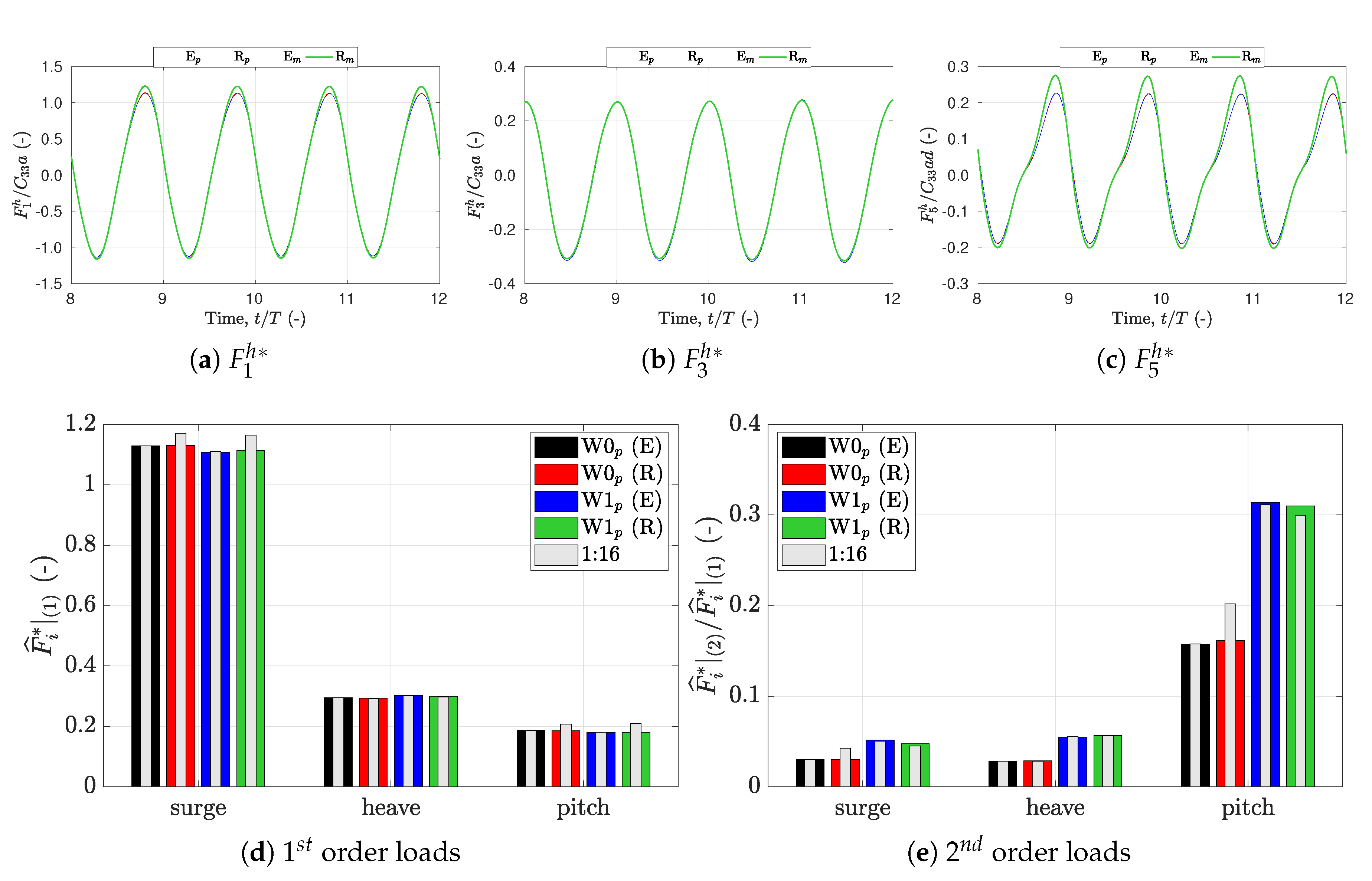
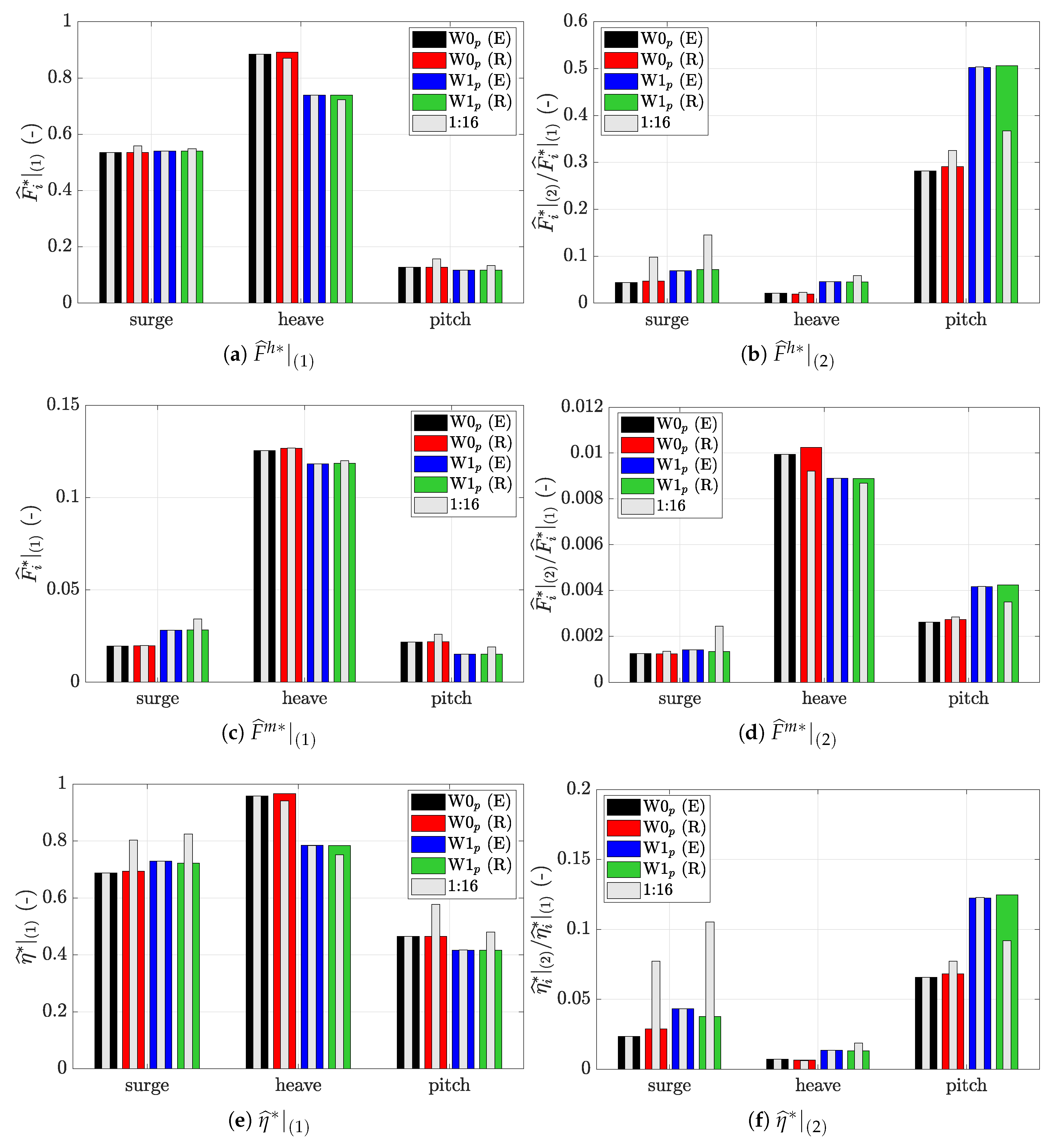
Although the WEC is allowed to move in six degrees-of-freedom (DoF), only the surge, heave and pitch modes of motion are excited by the long-crested waves studied in this paper. The results are therefore presented in terms of forces in surge, heave and pitch ($F_1,F_3,F_5$) and motions in surge, heave and pitch (${\eta }_1,{\eta }_3,{\eta }_5$). A hat $\left(\widehat{·}\right)$ denotes force or motion amplitude from the Fourier decomposition of the time signal. The first harmonic (or order) refers to the wave frequency, while the second order effects are in twice the wave frequency.

4.1. Non-Dimensionalisation

Results are presented in non-dimensional form according to the quantities described in

Table 4. Overview of the non-dimensionalisation factors used in results.

Factor	Description	Unit	Quantities
a	Incoming wave amplitude	m	${\eta }_1$, ${\eta }_3$
$ak$	Maximum wave slope	deg	${\eta }_5$
$C_{33}a$	Hydrostatic heave stiffness × wave amplitude	N	$F_1$, $F_3$
$C_{33}ad$	Hydrostatic heave stiffness × wave amplitude × diameter	Nm	$F_5$
T	Wave period	s	t

The heave stiffness for a cylinder reads $C_{33}=\pi \rho g{D}^2/4$

. Throughout the paper non-dimensional quantities are marked with an asterisk (${}^{*}$).

4.2. Wave Load Cases

The WEC is subjected to regular 5th order Stokes waves of period $T=5$ s in prototype scale, which is very close to the heave resonance period [31]. Two wave heights are studied, corresponding to steepness $H/L=2.5$% and $H/L=5$%. See

Table 5. Details on the regular wave cases studied. T is period time, L is the wave length (from k), a is wave amplitude and k is the wave number computed from linear theory.

Label	T (s)	a (m)	k (rad/m)	$\mathit{ak}$ (rad)	L (m)	$2\mathit{a}/\mathit{\lambda }$ (%)	KC (-)	Re (-)
W0 (1:1)	5	0.488	0.16	0.08	39.0	2.5	6.131 × 10${}^{-1}$	2.516 × 10${}^6$
W1 (1:1)	5	0.976	0.16	0.16	39.0	5.0	1.226	5.032 × 10${}^6$
W0 (1:16)	0.313	3.05 × 10${}^{-2}$	2.56	0.08	2.437	2.5	6.131 × 10${}^{-1}$	3.931 × 10${}^4$
W1 (1:16)	0.313	6.10 × 10${}^{-2}$	2.56	0.16	2.437	5.0	1.226	7.862 × 10${}^4$

for more details on the wave cases. Reference to a wave case will in the remainder of the paper be given by its label W0 or W1, where W0 is the more linear wave and W1 is the steeper wave. The wave period is chosen to be well inside the region of heave resonance of the WEC in order to study the nonlinear content of the interaction between wave forces and WEC motions.

4.3. Meshing for Wave Propagation

A two-dimensional wave tank was first implemented to check the mesh resolutions for any differences in wave propagation. The results are compiled in

Table 6. Wave propagation tests in a two-dimensional NWT. Results are for the RANS simulations. Euler results are within $\pm 0.0001a$ of the RANS results for all cases studied. ${\widehat{\zeta }}^{*}$ is nondimensionalised wave amplitude, $\delta \alpha /a$ is the non-dimensional interface spread between the iso-lines of $\alpha =0.95$ and $\alpha =0.05$.

Wave	Mesh	${\widehat{\mathit{\zeta }}}^{*}{|}_{(1)}$	$\mathit{\delta }\mathit{\alpha }/\mathit{a}$	${\widehat{\mathit{\zeta }}}^{*}{{|}_{(2)}/{\widehat{\mathit{\zeta }}}^{*}|}_{(1)}$
W0	M0	0.995	0.651	0.040
W0	M1	0.995	0.582	0.039
W0	M2	0.998	0.367	0.039
W1	M0	0.991	0.298	0.080
W1	M1	0.995	0.275	0.081
W1	M2	0.995	0.184	0.080

based on a Fourier transform of the wave elevation two wavelengths from the inlet at the location of the absent WEC, i.e., $(x,y)=(0,0)$ m. The wave was sampled 200 times per wave period. The M2 results were also verified in the full 3D NWT with no WEC present. The first order wave height at the WEC location is well predicted by all three mesh resolutions, with differences below $0.004a$. We conclude that all meshes are capable of transmitting sufficient wave energy from the inlet to the WEC, although the sharpness of the interface is clearly very much improved by increasing the cell density (see the $\delta \alpha /a$ value in Table 6). The nonlinear content of the waves can be quantified by the second order content of the amplitude spectrum shown in the last column of Table 6. Second harmonic content increases from 4% of the first order amplitude in W0 to 8% in W1. This is interesting to keep in mind when we compare the high-order contributions of the WEC loading later.

4.4. Meshing for Response

A mesh sensitivity study was made on the W1 case for the moored full-scale WEC in operation. Figure 3 shows the resulting time history of the three meshes. All three meshes agree on the predicted heave and pitch motions, but the coarsest mesh outputs a larger surge offset than the finer grids. The restoring mooring force is of low frequency with a small damping, which results in the long-lived initial transient seen in Figure 3a. A ramp time of 8 wave periods was put on the incident wave amplitude to keep this effect within acceptable amplitudes, but for the purpose of the current investigation we have chosen to accept a remainder of low frequency surge oscillation to save computational time. The transients in heave and pitch are quickly damped by the hydrodynamics and they quickly enter harmonic or bi-harmonic behaviour after the ramp period, as can also be seen from Figure 3. In order to obtain high resolution on flow details surrounding the WEC, the remainder of the results in this paper are from the finest (M2) mesh resolution.

Geometric similitude was used to scale the meshes, which in practice rendered a difference in resolution of the boundary layer due to the scaling factors. In the RANS simulations of the W1 wave, the prototype results had approximately $y_{max}^{+}\approx 80$ and the model scale results had approximately $y_{max}^{+}\approx 10$.

4.5. Fixed and Moored Simulations

In the fixed simulations the stationary WEC was held at the moored equilibrium position from Table 1, so that the mesh was statically morphed according to a draft of $5.63$ m.

Preliminary tests of the moored WEC showed a small but notable force in the span-wise direction, which was found to be caused by reflections from the side walls [45]. Although it was too small to affect the surge, heave and pitch response, we chose to simulate the moored WEC in a significantly widened tank to avoid any pollution of the results from the side walls. The blockage factor in the span-wise direction was decreased from 5/65 = 0.077 in the narrow tank, to 5/160 = 0.031 in the widened tank.

5. Results

This section presents the main results of the simulation campaign. Results from both fixed WEC and moored WEC simulations are presented for each of the two scales.

5.1. Prototype Results

The fixed WEC results are presented with hydrodynamic force amplitudes in

Table 7. Prototype scale force amplitudes for the fixed WEC. $\left({\widehat{F}}_i^{*}{|}_{(k)}\right)$ denotes the $k^{th}$ order amplitude in mode i. Simulation types are headlined: R for RANS; E for Euler; and L for linear. See Table 4 for non-dimensionalisation factors.

Wave	Type	${\widehat{\mathit{F}}}_1^{*}{|}_{(1)}$	${\widehat{\mathit{F}}}_3^{*}{|}_{(1)}$	${\widehat{\mathit{F}}}_5^{*}{|}_{(1)}$	${\widehat{\mathit{F}}}_1^{*}{|}_{(2)/(1)}$	${\widehat{\mathit{F}}}_3^{*}{|}_{(2)/(1)}$	${\widehat{\mathit{F}}}_5^{*}{|}_{(2)/(1)}$
W0	R	1.131	0.294	0.186	0.030	0.029	0.161
W0	E	1.129	0.295	0.187	0.030	0.028	0.157
W0	L	1.168	0.293	0.190	0.030	0.000	0.115
W1	R	1.113	0.299	0.180	0.047	0.056	0.310
W1	E	1.109	0.302	0.181	0.052	0.055	0.314
W1	L	1.166	0.291	0.192	0.061	0.001	0.227

. The forces agree very well across all three computational methods for first order heave and pitch response, but the linear method has a lower amplitude of second order content compared with the RANS and Euler results. In surge, the force is linear with respect to wave steepness, but the linear method gives approximately 4% larger force. The first order heave force amplitude is between 0.291 and 0.302. Clearly the heave force amplitude is linear with respect to wave steepness and the diffraction problem of a vertical cylinder is well captured by a linear radiation-diffraction approach. The errors of the linear results are dominated by the missing second order heave contribution, which is very close to the steepness of the wave case for both W0 and W1.

The moored WEC results are presented as motion amplitudes in

Table 8. Prototype scale motion amplitude response for the moored WEC. $\left({\widehat{\eta }}_i^{*}{|}_{(k)}\right)$ denotes the $k^{th}$ order amplitude of motion mode i. Simulation types are headlined: R for RANS; E for Euler; and L for linear. See Table 4 for non-dimensionalisation factors.

Wave	Type	${\widehat{\mathit{\eta }}}_1^{*}{|}_{(1)}$	${\widehat{\mathit{\eta }}}_3^{*}{|}_{(1)}$	${\widehat{\mathit{\eta }}}_5^{*}{|}_{(1)}$	${\widehat{\mathit{\eta }}}_1^{*}{|}_{(2)/(1)}$	${\widehat{\mathit{\eta }}}_3^{*}{|}_{(2)/(1)}$	${\widehat{\mathit{\eta }}}_5^{*}{|}_{(2)/(1)}$
W0	R	0.694	0.966	0.465	0.029	0.007	0.068
W0	E	0.688	0.958	0.465	0.023	0.007	0.066
W0	L	0.723	1.066	0.519	0.032	0.009	0.089
W1	R	0.723	0.784	0.417	0.038	0.013	0.125
W1	E	0.729	0.785	0.417	0.043	0.014	0.122
W1	L	0.761	1.036	0.591	0.066	0.015	0.164
W1/W0	R	1.042	0.812	0.897	1.310	1.857	1.838
W1/W0	E	1.060	0.819	0.897	1.870	2.000	1.849
W1/W0	L	1.053	0.972	1.139	2.063	1.667	1.843

. The Euler and the RANS results agree very well across the signals, but the linear motion results are significantly larger in first order amplitudes than the corresponding CFD (i.e., both Euler and RANS) results. In heave this effect is 10% for W0 and 24% for W1. The trend in moving from W0 to W1 is the same for all simulations in heave and surge, where the surge amplitude is increasing and the heave amplitude is decreasing, although to a much larger extent in the CFD results. In pitch however, the RAO increases for larger waves using the linear approach, while it is decreasing somewhat in the CFD simulations. The most important result in this context is that the heave RAO decreases due to increased wave height. The decrease is only 3% using the linear method, while both Euler and RANS give an 18–19% reduction.

Further, Table 8 shows that the second order content is most evident in pitch, with contributions of roughly 12% of the first order amplitude for CFD, and 16% for the linear model. The heave response is completely dominated by the first order response and second harmonic content is below 2% for W1. Although still small, we note that the second harmonic contribution of all responses grows with the wave height, increasing from e.g., 0.7–1.4% in heave response between W0 to W1.

5.2. Scale Effects

The top row of Figure 4 shows the force time history on the fixed WEC in both model and prototype scale. The first and second harmonic amplitudes are also presented in the bottom row bar charts of Figure 4. The same linear trend with respect to wave height is seen in the model scale results. We note negligible scale effects in heave response but see a minor viscous contribution in surge and pitch excitation, which experience a slight increase in the model scale compared with the prototype. We also note that the Euler simulations are, as expected, independent of scale.

Figure 5 and Figure 6 present the model and prototype scale results of the CFD simulations for the moored WEC. As in the fixed case of Figure 4, all Euler results are consistently scale-independent also in the moored case. For the RANS results however, the surge direction is sensitive to scale, which gives both an increased first order amplitude in Figure 6 and an increased maximum drift offset in Figure 5. Heave is less affected by the shift in scale, but the model scale RANS results are 2.5% lower than the prototype scale for W0, and 4.2% lower in W1. Due to the closeness of the RANS and Euler response in prototype scale, similar values are obtained for the pure viscous difference between RANS and Euler simulations in model scale (1.7% for W0 and 4.2% for W1). The relative reduction of RAO from W0 to W1 in model scale RANS is however similar to the full-scale results in Table 8. So we conclude that the 18–19% reduction seen in the heave RAO is scale-independent, and that a 1–4% reduction due to purely viscous drag is applicable for the model scale case.

5.3. Heave Analysis

In this section we present a detailed analysis of the loss of heave RAO between wave heights. Figure 7 shows the decomposition of the total dynamic force in heave due to hydrodynamics, moorings and power take-off. The hydrostatic heave force component $\left(C_{33}{\eta }_3\right)$ has been subtracted from the hydrodynamic force. Two additional RANS simulations with heave only were made in prototype scale to identify the effects of surge and pitch on the heave results. These results are also presented in Figure 7.

From the power take-off force ($F_{\mathrm{pto}}$), we can compute the mean power extraction

$$\begin{array}{cc}\hfill \overline{P}& ={\displaystyle \frac{1}{T}}{\int }_T{F}_{\mathrm{pto}}(t)v(t)\mathrm{dt}.\hfill \end{array}$$

(8)

If normalised with the square of the wave amplitude, it shows that the power output due to the decreasing RAO drops from $\overline{P}/a^2=11.04$ kW/m${}^2$ in W0 to $\overline{P}/a^2=7.34$ kW/m${}^2$ in W1 for the moored RANS prototype simulations, a decrease with 33%. The power take-off and the mooring forces are of similar amplitudes, where both forces contribute significantly to the damping of the heave motion, see preliminary work in [46]. However, by comparing the heave only results of Figure 7 to the fully moored cases we note that the only clear differences seen between mooring forces in W0 and W1 are due to the slight surge offset between the cases. Hence, the moorings are not the cause of the RAO loss from Figure 6, and neither is the PTO. The PTO force is a pure linear damper, and the relative amplitude loss in PTO force in the W1 wave is simply the consequence of a reduced RAO. A comparison between the hydrodynamic force in RANS and Euler results shows that the surge phase difference is shifting the response in time, but that the peak values of the forces are very similar across the simulation types. The viscous influence is most evident around $t=12.5T$ for all W1 cases. RANS simulations give an extra oscillation here, where the Euler simulations show more of a plateau in the force. Consequently, there is a clear difference around the negative peak amplitude between W0 and W1 simulations. The results can be discussed further based on the pressure distribution underneath the buoy.

Figure 8 shows the Q = 200 iso-surface and the dynamic pressure on the bottom of the fixed buoy in the W1 RANS model scale simulation over one wave period. It is easy to follow the progression of the incoming wave pressure and its relatively smooth variation over the bottom surface as time progresses. Please note that Table 7 shows that the heave force amplitude of this case is linear with respect to wave steepness.

When the WEC is moored and allowed to move, the Q = 200 iso-surface shown in Figure 9 presents coherent vortex tubes below or around the body during both upward and downward motion of the WEC. A vortex torus is formed underneath the buoy during the upward motion. The upward motion is shown in the top line of Figure 9, where Q has been colored in red for a clock-wise rotating vorticity vector (seen from below). The vortex is detached and follows the buoy until it reaches the top position. As the WEC turns, the torus radius increases and the vorticity decreases until it dissolves on the side of the buoy. During the downward motion, a counter-rotating torus (see blue surfaces in Figure 9) is generated on the side of the buoy as water underneath is pushed towards the outside. Also these vortices separate from the buoy and dissolve away from the buoy. The geometry of the rotating flow regions are consistent with those previously reported [6,23,25].

The presence of the vortices correspond very well to a local variation of pressure underneath the buoy. The effect of the vortex structures is clearly seen in the dynamic pressure distribution on the bottom plate of the cylinder shown in the bottom row of Figure 9. Figure 10 provides a qualitative comparison of the effect of the vortex on the pressure field beneath the WEC by snap shots of the 0.1 iso-pressure contour around the peak of the hydrodynamic force in Figure 7 (0.2 T into the wave period). Also shown is the corresponding pressure distribution under the buoy. The clearest effect is between wave heights, where the W1 waves consistently show larger, more coherent and stronger pressure tubes than the W0 results. We also highlight the similar vortex structures seen in the Euler and the RANS simulations at both scales, which enforces the induced drag term as scale independent and geometrically induced. The vortex regions are acting obtrusively on the dynamic pressure field of the wave so that a smaller portion of the bottom area is subjected to the driving wave force, which in turn can cause the loss of RAO with increasing wave height shown in Figure 6c. The vorticity of the flow also adds to the inertial effects of the surrounding water, which may be the cause of the plateau of hydrodynamic force around $t=12.5T$ in Figure 7.

6. Discussion

The scale effects of WECs are connected to the viscous contribution and the incompatibility of Reynolds scaling and Froude scaling. For oscillating systems, the importance of viscous forces in relation to inertial forces is traditionally determined by the Keulegan–Carpenter number (KC) [27,47]. However, KC is typically defined with respect to an oscillating fluid or an oscillating body in still water, so that an expected relative velocity can be easily obtained from the maximum velocity of the loading. For PAWECs it is more complicated. The actual KC number comes from the maximum relative velocity in each cycle of the case, which depends on the phase lag between the wave particle motion and the WEC response. Obviously these relative velocities also depend on the power take-off and the control of the device. As an example we refer to [29] where the relevant KC number for acceptable Froude scaling accuracy of an oscillating wave surge converter was transformed from 10 in pitch decay to 4.18 for response in waves. The surge force is also in this paper the most prone to effects of scale. Figure 6 shows the scale effect on both surge force and surge amplitude response, while the Euler simulations agree well with the RANS results in prototype scale. There is some uncertainty in the surge (and pitch) results due to the numerical treatment of the boundary layer in the near-wall region. First, the VOF method of a free surface near the WEC hull can cause fractions of air to get stuck on the wall due to the no-slip condition. This can cause a pressure disturbance as the wave crest passes. The slip condition in the Euler simulation has no problems of this kind, despite the continued use of a boundary layer mesh. Then, there is the question of wall functions in oscillating flow. Both Schmitt & Elsaesser [28] and Gu et al. [20] highlight the difficulty of boundary layer treatment at different scales. Our choice of wall functions are continuously shifting over low-RE to high-RE for the turbulent viscosity, while remaining high-RE for the kinetic energy and the dissipation rate. The shear forces in all simulations are however very small, as was also reported by Gu et al. [20]. They also achieved good surge force results regardless of a trailing shear force resolution dependence. In light of this, we consider the surge mode to be adequately modelled. However, increasing the fidelity of RANS surge models at model-scale is a very important topic for further investigations, particularly from the perspective of mooring design. A good surge model is essential to a good validation and design of the mooring system and the survivability of the WEC, as was observed by Harnois et al. [48] when comparing numerical results to both controlled tank test data and to more uncertain field test data. Understanding the model scale effects in all modes of motion is imperative for mooring designs based on wave-to-wire simulations calibrated with tank test data in smaller scales. An overestimation of the surge loads results in stiffer moorings (for the same maximum allowed offset) which are typically more expensive and give rise to larger forces than more compliant systems.

The WEC is a truncated vertical cylinder, whose flat bottom is generally regarded as the bottom shape most affected by drag damping effects in the heave direction [7,20,30]. The results of induced drag influence in this paper should therefore be considered as higher than more realistic designs. As the RAO increases (which a better PAWEC design should accomplish) the importance of drag damping from the wall-shear stress increases and larger differences between Euler and RANS simulations can be obtained. These differences will then be the subject of scaling effects as they will scale with the Reynolds number.

We argue that a combined analysis using both VOF-Euler and VOF-RANS simulations provides a powerful tool for understanding how a WEC concept behaves at different scales and conditions. Vast experience with Euler simulations on air-craft wings has showed that although vortex generation is triggered by the existence of a numerical viscosity, the results are rather insensitive to its magnitude [49]. Therefore, we argue that as the heave motion was insensitive to mesh resolution, and as the drag damping is shown to be dominated by the induced drag also captured by the Euler simulations, the vortex formation is reasonably well modelled in this paper. Our results show that the Euler simulations are indeed scale-independent and therefore they can be used to quantify the uncertainties due to viscosity and scale of the device. As the scale increases, the viscous influence decreases and the results of Euler and RANS simulations start to converge. As such, when validating CFD simulations to model scale experiments, the RANS results should be in good agreement with the physical model. If so, an Euler simulation using the same mesh can be used to separate the drag influence into a scale-dependent viscous part and a near inviscid scale-independent part. For the same reason, the difference between Euler and RANS results at model scale provides an upper bound on the viscous effects on the WEC concept.

7. Conclusions

The paper has shown how combined VOF-RANS and VOF-Euler simulations can be used to analyse viscous effects and effects of scale on a generic moored point-absorber wave energy converter (PAWEC). Using dynamic mooring simulations via a coupled finite element solver and a linear power take off, the studied case represents a highly realistic scenario for slack-moored PAWECs. This type of analysis is of particular importance for CFD studies aimed at producing drag coefficients for use in wave-to-wire models. A thorough analysis of the underlying factors of the drag force can for a given geometry provide valuable understanding of the design and improve the device performance at a desired scale.

We have focused on a very simple geometry studied in the resonance region. The conclusions and results below should therefore be considered as indicative for this particular case. Obviously the numbers and percentages will differ significantly upon changing the device geometry, its mooring design or indeed increasing its PTO complexity. Below we list the main results and findings of the simulation campaign. For brevity we refer to W0 and W1 as the regular wave cases of 2.5% and 5% steepness, respectively.

• First order hydrodynamic forces scale linearly with wave height for a fixed WEC. No viscous effects are seen in the full scale prototype, but scale effects are observed via increased surge force and pitch moment in the model scale RANS simulation. The method error of using a linear model to compute the heave diffraction problem is contained in the second harmonic and is of the same order as the steepness of the waves, i.e., 2.8% for W0 and 5.5% for W1.
• Euler simulations of both fixed and moored WECs are scale independent, also in the presence of induced drag forces from vortex formation surrounding the sharp bottom edge of the truncated cylinder.
• Compared to the linear simulation, the CFD prototype heave amplitudes are 10% and 24% smaller for W0 and W1, respectively, attributed mainly to drag forces.
• Doubling the wave steepness reduces the heave RAO by 3% due to moorings and Froude–Krylov forces, by some 1–4% due to viscous effects in model scale, and by 18–19% due to induced drag and other nonlinearities.
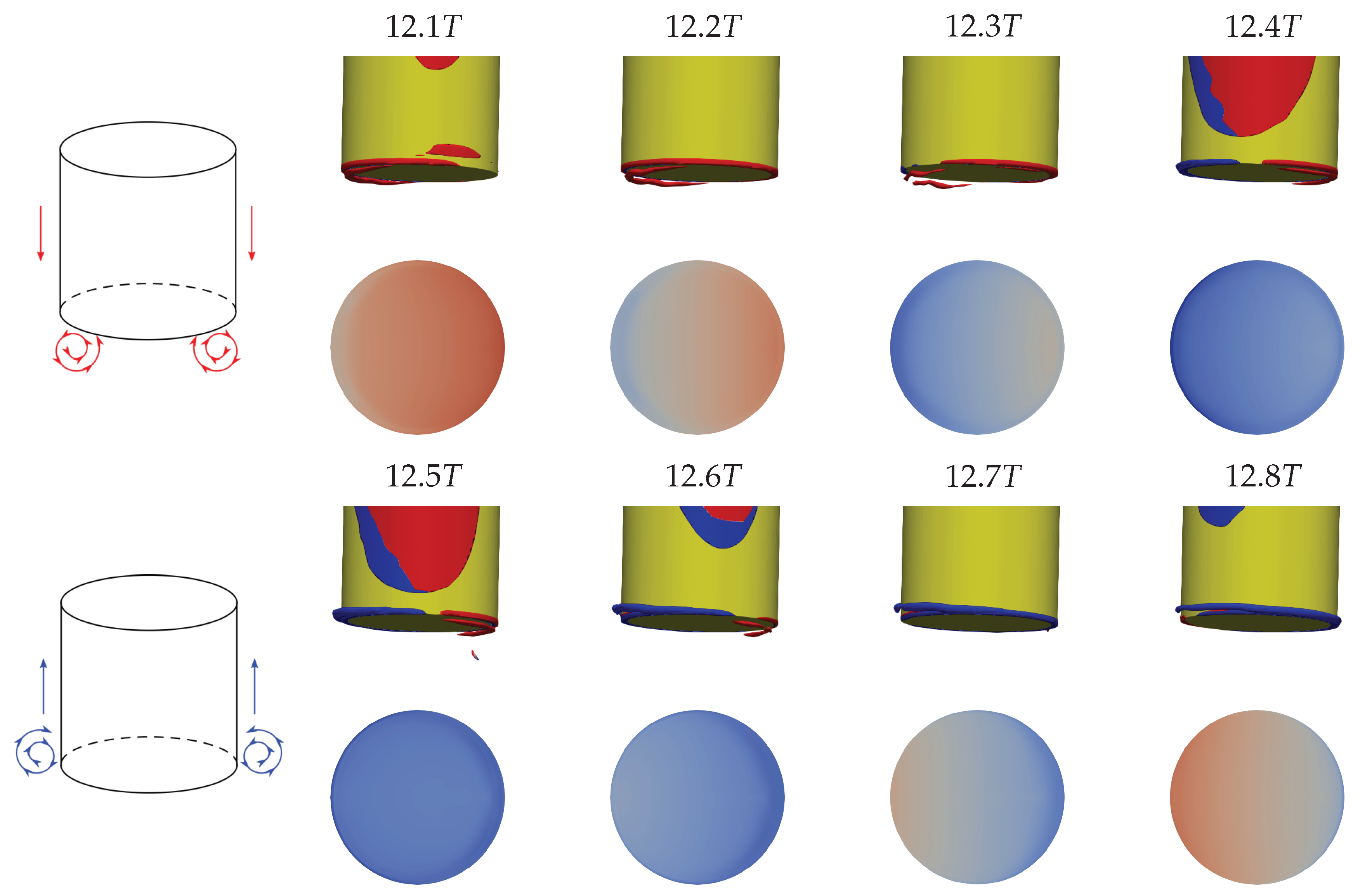
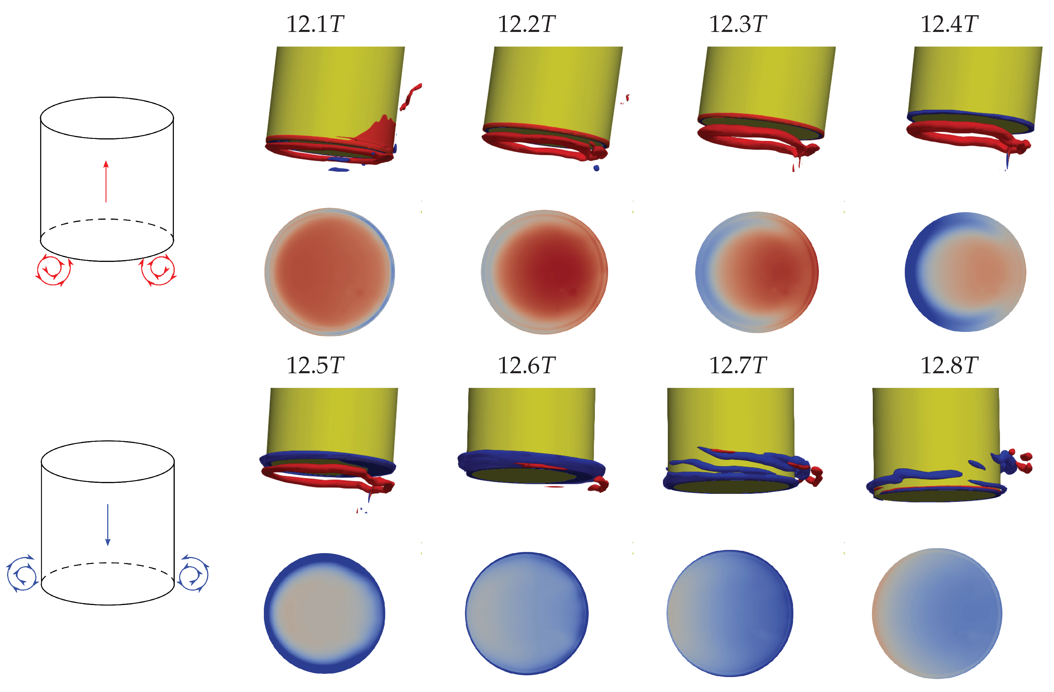
• The heave drag force is clearly affected by scale-independent induced drag effects. Via analysis of the pressure distribution surrounding the bottom of the WEC, we show that the induced drag is caused by regions of low pressure from vortex tubes underneath the buoy. The vorticity of the flow affects the driving wave pressure and prevents it from acting on the whole area of the buoy, which reduces the wave force amplitude.
• Scale effects are most dominant in the surge direction of the RANS simulation. There are uncertainties in the results due to the numerical treatment of the boundary layer in the VOF method, and due to the use of wall-functions in oscillatory flow. More numerical development is needed to avoid these issues and ascertain high-fidelity surge forces.

Based on the results obtained in this study we argue that the use of calibrated drag correction coefficients can be suitable for all scales of a device if it has regions of sharp pressure gradients (such as the sharp corner of the truncated cylinder in this study). In these cases the scale-independent induced drag is the dominating drag influence and the viscous part is less important. For smoother geometries, another relation between viscous and induced drag applies. We recommend that both RANS and Euler simulations are used during numerical validation against experimental model scale tests in order to separate the viscous drag influence from the induced drag. Consequently, this approach can be used to quantify the effects of scale on wave energy converters.

References

1. Pecher, A.; Kofoed, J.P. Handbook of Ocean Wave Energy; Springer: Berlin, Germany, 2017. [Google Scholar]
2. Fitzgerald, J.; Bolund, B. Technology Readiness for Wave Energy Projects; ESB and Vattenfall classification system. In Proceedings of the 4th International Conference on Ocean Energy, Dublin, Ireland, 17–19 October 2012. [Google Scholar]
3. Windt, C.; Davidson, J.; Ringwood, J. High-fidelity numerical modelling of ocean wave energy systems: A review of computational fluid dynamics-based numerical wave tanks. Renew. Sustain. Energy Rev. 2018, 93, 610–630. [Google Scholar] [CrossRef]
4. Yu, Y.; Li, Y. Reynolds-Averaged Navier-Stokes simulation of the heave performance of a two-body floating-point absorber wave energy system. Comput. Fluids 2013, 73, 104–114. [Google Scholar] [CrossRef]
5. Chen, L.; Zang, J.; Hillis, A.; Morgan, G.; Plummer, A. Numerical investigation of wave-structure interaction using OpenFOAM. Ocean Eng. 2014, 88, 91–109. [Google Scholar] [CrossRef] [Green Version]
6. Palm, J.; Eskilsson, C.; Paredes, G.; Bergdahl, L. Coupled mooring analysis for floating wave energy converters using CFD: Formulation and validation. Int. J. Mar. Energy 2016, 16, 83–99. [Google Scholar] [CrossRef]
7. Chen, Z.; Zhou, B.; Zhang, L.; Zhang, W.; Wang, S. Geometrical Evaluation on the Viscous Effect of Point-Absorber Wave-Energy Converters. China Ocean Eng. 2018, 32, 443–452. [Google Scholar] [CrossRef]
8. Penalba, M.; Davidson, J.; Windt, C.; Ringwood, J.V. A high-fidelity wave-to-wire simulation platform for wave energy converters: Coupled numerical wave tank and power take-off models. Appl. Energy 2018, 226, 655–669. [Google Scholar] [CrossRef]
9. Devolder, B.; Stratigaki, V.; Troch, P.; Rauwoens, P. CFD Simulations of Floating Point Absorber Wave Energy Converter Arrays Subjected to Regular Waves. Energies 2018, 11, 641. [Google Scholar] [CrossRef]
10. Wang, W.; Wu, M.; Palm, J.; Eskilsson, C. Estimation of numerical uncertainty in CFD simulations of a passively controlled wave energy converter. Proc. Inst. Mech. Eng. Part M J. Eng. Marit. Environ. 2018, 232, 71–84. [Google Scholar]
11. Coe, R.; Neary, V. Review of methods for modeling wave energy converter survival in extreme sea states. In Proceedings of the 2nd Marine Energy Technology Symposium, Seattle, WA, USA, 15–18 April 2014. [Google Scholar]
12. Wolgamot, H.; Fitzgerald, C. Nonlinear hydrodynamic and real fluid effects on wave energy converters. Proc. Inst. Mech. Eng. Part A J. Power Energy 2015, 229, 772–794. [Google Scholar] [CrossRef]
13. Davidson, J.; Giorgi, S.; Ringwood, J. Linear parametric models for ocean wave energy converters identified from numerical wave tank experiments. Ocean Eng. 2015, 103, 31–39. [Google Scholar] [CrossRef]
14. Giorgi, S.; Ringwood, J. Comparing nonlinear hydrodynamic forces in heaving point absorbers and oscillating wave surge converters. J. Ocean Eng. Mar. Energy 2017, 4, 25–35. [Google Scholar] [CrossRef]
15. Morison, J.; O’Brien, M.; Johnson, J.; Schaaf, S. The Force Exerted by Surface Waves on Piles. J. Pet. Technol. 1950, 186, 149–154. [Google Scholar] [CrossRef]
16. Rodrigues, M.; Spinneken, J. A laboratory study on the loading and motion of a heaving box. J. Fluids Struct. 2016, 64, 107–126. [Google Scholar] [CrossRef]
17. Rodrigues, M.; Spinneken, J.; Swan, C. Nonlinear loading of a two-dimensional heaving box. J. Fluids Struct. 2016, 60, 80–96. [Google Scholar] [CrossRef] [Green Version]
18. Bhinder, M.; Babarit, A.; Gentaz, L.; Ferrant, P. Potential time domain model with viscous correction and CFD analysis of a generic surging floating wave energy converter. Int. J. Mar. Energy 2015, 10, 70–96. [Google Scholar] [CrossRef]
19. Stansby, P.; Gu, H.; Moreno, E.; Stallard, T. Drag minimisation for high capture width with three float wave energy converter M4. In Proceedings of the 11th European Wave and Tidal energy Conference, Nantes, France, 6–11 September 2015. [Google Scholar]
20. Gu, H.; Stansby, P.; Stallard, T.; Carpintero Moreno, E. Drag, added mass and radiation damping of oscillating vertical cylindrical bodies in heave and surge in still water. J. Fluids Struct. 2018, 82, 343–356. [Google Scholar] [CrossRef]
21. Giorgi, S.; Ringwood, J. Importance of Nonlinear Wave Representation for Nonlinear Froude–Krylov Force Calculations for Wave Energy Devices. In Proceedings of the 12th European Wave and Tidal Energy Conference, Cork, Ireland, 27 August–1 September 2017. [Google Scholar]
22. Giorgi, S.; Ringwood, J. Nonlinear Froude–Krylov and viscous drag representations for wave energy converters in the computation/fidelity continuum. Ocean Eng. 2017, 141, 164–175. [Google Scholar] [CrossRef]
23. Jin, S.; Patton, R.; Guo, B. Viscosity effect on a point absorber wave energy converter hydrodynamics validated by simulation and experiment. Renew. Energy 2018, 124 Pt A, 500–512. [Google Scholar] [CrossRef]
24. Det Norske Veritas. DNV-RP-C205: Envirnonmental Conditions and Environmental Loads; Det Norske Veritas: Høvik, Norway, 2010. [Google Scholar]
25. Longbin Tao, L.; Thiagarajan, K. Low KC flow regimes of oscillating sharp edges I. Vortex shedding observation. Appl. Ocean Res. 2003, 25, 21–35. [Google Scholar]
26. Wei, Y.; Rafiee, A.; Henry, A.; Dias, F. Wave interaction with an oscillating wave surge converter, Part I: Viscous effects. Ocean Eng. 2018, 104, 185–203. [Google Scholar] [CrossRef]
27. Sarpkaya, T.; Isaacson, M. Mechanics of Wave Forces on Offsore Structures; Van Nordstrand Reinhold: New York, NY, USA, 1981. [Google Scholar]
28. Schmitt, P.; Elsaesser, B. The application of Froude scaling to model tests of Oscillating Wave Surge Converters. Ocean Eng. 2017, 141, 108–115. [Google Scholar] [CrossRef]
29. Pathak, A.; Freniere, C.; Raessi, M. Advanced computational simulations of water waves interacting with wave energy converters. Eur. J. Comput. Mech. 2017, 26, 172–204. [Google Scholar] [CrossRef]
30. Stansby, P.; Carpinteno Moreno, E.; Stallard, T. Capture width of the three-float multi-mode multi-resonance broadband wave energy line absorber M4 from laboratory studies with irregular waves of different spectral shape and directional spread. J. Ocean Eng. Mar. Energy 2015, 1, 287–298. [Google Scholar] [CrossRef] [Green Version]
31. Fitzgerald, J.; Bergdahl, L. Including moorings in the assessment of a generic offshore wave energy converter: A frequency domain approach. Mar. Struct. 2008, 21, 23–46. [Google Scholar] [CrossRef]
32. Bergdahl, L.; Palm, J.; Eskilsson, C.; Lindahl, J. Dynamically Scaled Model Experiment of a Mooring Cable. J. Mar. Sci. Eng. 2016, 4, 5. [Google Scholar] [CrossRef]
33. OpenCFD Ltd. OpenFOAM Homepage; 2014. Available online: http://www.openfoam.org (accessed on 1 December 2014).
34. Weller, H.; Tabor, G.; Jasak, H.; Fureby, C. A tensorial approach to CFD using object oriented techniques. Comput. Phys. 1998, 12, 620–631. [Google Scholar] [CrossRef]
35. Jacobsen, N.; Fuhrman, D.; Fredsoe, J. A wave generation toolbox for the open-source CFD-library OpenFOAM. Int. J. Numer. Meth. Fluids 2012, 70, 1073–1088. [Google Scholar] [CrossRef]
36. Palm, J.; Paredes, G.; Eskilsson, C.; Taveira-Pinto, F.; Bergdahl, L. Simulation of mooring cable dynamics using a discontinuous Galerkin method. In Proceedings of the 5th International Conference on Computational Methods in Marine Engineering, Hamburg, Germany, 29–31 May 2013. [Google Scholar]
37. Palm, J. Mooring Dynamics for Wave Energy Applications. Ph.D. Thesis, Chalmers University of Technology, Gothenburg, Sweden, 2017. [Google Scholar]
38. Yakhot, V.; Orszag, S.; Thangam, S.; Gatski, T.; Speziale, C. Development of turbulence models for shear flows by a double expansion technique. Phys. Fluids A 1992, 4, 1510–1520. [Google Scholar] [CrossRef] [Green Version]
39. Spalart, P. Airplane Trailing Vortices. Annu. Rev. Fluid Mech. 1998, 30, 107–138. [Google Scholar] [CrossRef]
40. Yang, S.; Luo, S.; Liu, F. Euler Solutions of Flow around a Rectangular Wing with Square Tip. In Proceedings of the 45th AIAA Aerospace Sciences Meeting and Exhibit, Reno, NV, USA, 8–11 January 2007. [Google Scholar]
41. Palm, J.; Eskilsson, C. MOODY, User’s Manual Version m-1.0. 2014. Available online: www.sdwed.civil.aau.dk (accessed on 1 January 2015).
42. ANSYS Inc. AQWA Theory Manual 19.1; ANSYS Inc.: Canonsburg, PA, USA, 2018. [Google Scholar]
43. Lin, P.; Liu, P. A numerical study of breaking waves in the surf zone. J. Fluid Mech. 1998, 359, 239–264. [Google Scholar] [CrossRef]
44. Rusche, H. Computational Fluid Dynamics of Dispersed Two-Phase Flow at High Phase Fractions. Ph.D. Thesis, Imperial College London, London, UK, 2003. [Google Scholar]
45. Palm, J.; Eskilsson, C.; Bergdahl, L. Parametric excitation of moored wave energy converters using viscous and non-viscous CFD simulations. In Progress in Renewable Energies Offshore; Guedes Soares, C., Ed.; Taylor & Francis Group: Abingdon, UK, 2018; pp. 455–462. [Google Scholar]
46. Palm, J.; Eskilsson, C.; Paredes, G.; Bergdahl, L. CFD simulations of a moored floating wave energy converter. In Proceedings of the 10th European Wave and Tidal Energy Conference, Aalborg, Denmark, 2–5 September 2013. [Google Scholar]
47. Dean, R.; Dalrymple, R. Water Wave Mechanics for Engineers and Scientists; World Scientific: Singapore, 1991. [Google Scholar]
48. Harnois, V. Analysis of Highly Dynamic Mooring Systems: Peak Mooring Loads in Realistic Sea Conditions. Ph.D. Thesis, University of Exeter, Exeter, UK, 2014. [Google Scholar]
49. Fujii, K.; Gavali, S.; Holst, T. Evaluation of Navier–Stokes and Euler Solutions for leading-edge separation vortices. Int. J. Numer. Meth. Fluids 1988, 8, 1319–1329. [Google Scholar] [CrossRef]
Figure 1. Layout of the numerical wave tank. The WEC is in the origin and the four mooring cables are symmetrically placed along the xy coordinate axes.
Jmse 06 00124 g001
Figure 2. Overview of the discretised numerical wave tank: (a) global mesh; (b) morphing mesh region; and (c) discretisation of the body.
Jmse 06 00124 g002
Figure 3. Mesh dependence of motion response in (a) surge, (b) heave, and (c) pitch.
Jmse 06 00124 g003
Figure 4. Hydrodynamic forces acting on the fixed WEC. (ac) are time histories in the W1 wave. (d) is first order amplitudes, and (e) is second order amplitudes relative to the first order. Coloured bars are prototype results and thinner grey bars are the model scale (1:16) results. See Table 4 for non-dimensionalisation factors.
Jmse 06 00124 g004
Figure 5. Time histories of hydrodynamic forces (top row) and the motion response (bottom row) in W1 for Euler (E) and RANS (R) simulations at prototype (p) and model (m) scales.
Jmse 06 00124 g005
Figure 6. Euler (E) and RANS (R) results for the moored WEC in waves W0 and W1 showing first and second harmonic amplitudes in surge, heave and pitch. Top row shows hydrodynamic forces, middle row shows mooring forces and bottom row shows motion response. Left side is first order, and right side is second order. The coloured bars are prototype scale results, and the corresponding model scale (1:16) results are displayed as thinner grey bars. See Table 4 for non-dimensionalisation factors.
Jmse 06 00124 g006
Figure 7. Force decomposition depending on wave steepness (W0-solid lines, W1-dashed lines).
Jmse 06 00124 g007
Figure 8. Vortex formation and pressure distribution over a wave cycle in the fixed case. The Q = 200 iso-surface is colored by rotation direction (inward rotation is red and outward is blue, see schematics on the left). Top two rows are upward motion, bottom two rows are downward motion. The colour-scale of the pressure distribution goes from blue to red in [−0.5, 0.5] (-). The wave propagates from left to right in all figures.
Jmse 06 00124 g008
Figure 9. Vortex formation over the wave period T with corresponding dynamic pressure distribution on the bottom of the buoy for the W1 RANS model scale simulations. Vortices are visualized by the Q = 200 iso-surface and colored by rotation direction (inward rotation is blue and outward is red, see schematics on the left). Top two rows are upward motion, top bottom rows are downward motion. The colour-scale of the pressure distribution goes from blue to red in [−0.25, 0.25], in non- dimensionalised values. The wave propagates from left to right in all figures, while the positive y-direction is into the figure in the top row, and is directed downwards in the pressure plots.
Jmse 06 00124 g009
Figure 10. Pressure distribution at the y = 0 plane, including p ˜ = 0.1 iso-surface showing the extent of the vortex influence over dynamic pressure. p ˜ = ( p + ρ g z ) / ( ρ g a ) . Also shown is the corresponding pressure distribution on the WEC bottom. Results are from t * = 12.2 T for the Euler simulation and t * = 14.2 T for the RANS simulations. The colour scale is from blue to red [−0.1, 0.25].
Jmse 06 00124 g010