Wave and Tidal Controls on Embayment Circulation and Headland Bypassing for an Exposed, Macrotidal Site

 , ,
, , 
Abstract
1. Introduction
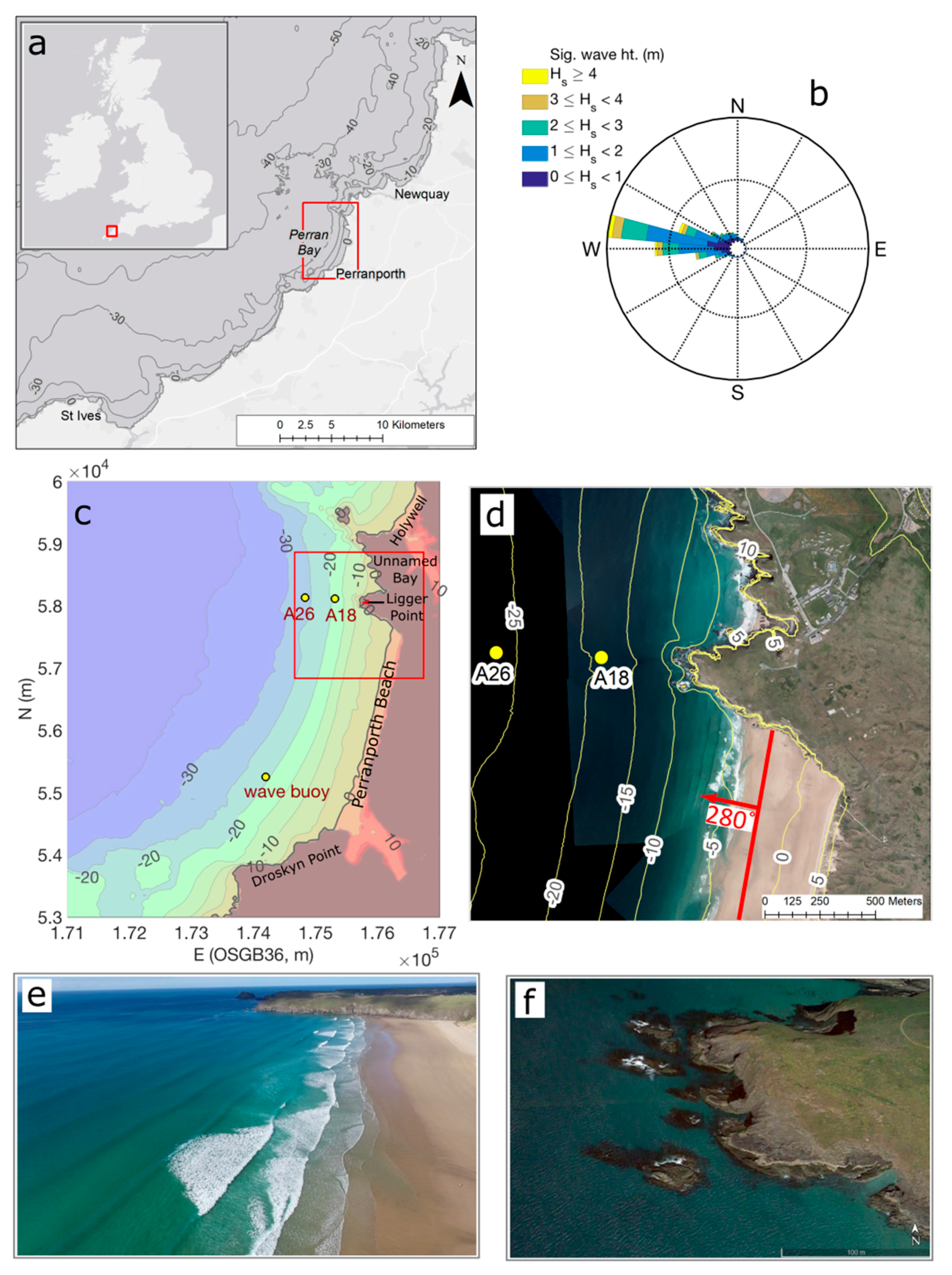
2. Study Site
3. Materials and Methods
3.1. Field Observations
3.1.1. Wave and Hydrodynamic Observations
3.1.2. Survey Data
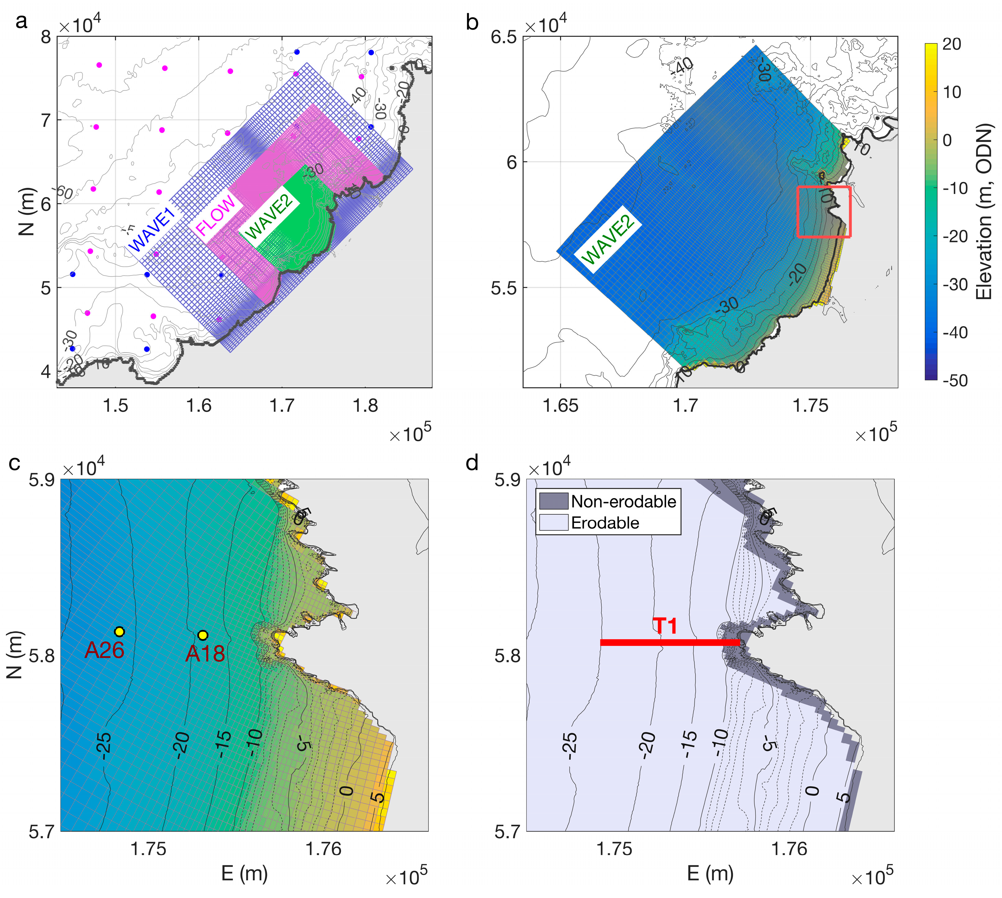
3.2. Numerical Modelling
3.2.1. Wave Model
3.2.2. Hydrodynamic Model
3.2.3. Wind and Pressure Inputs
3.2.4. Non-Erodible Layer
3.2.5. Model Calibration
3.2.6. Additional Synthetic Simulations
3.2.7. Headland Transect for Bypassing Analysis
3.2.8. Model Design Assumptions and Limitations
4. Results
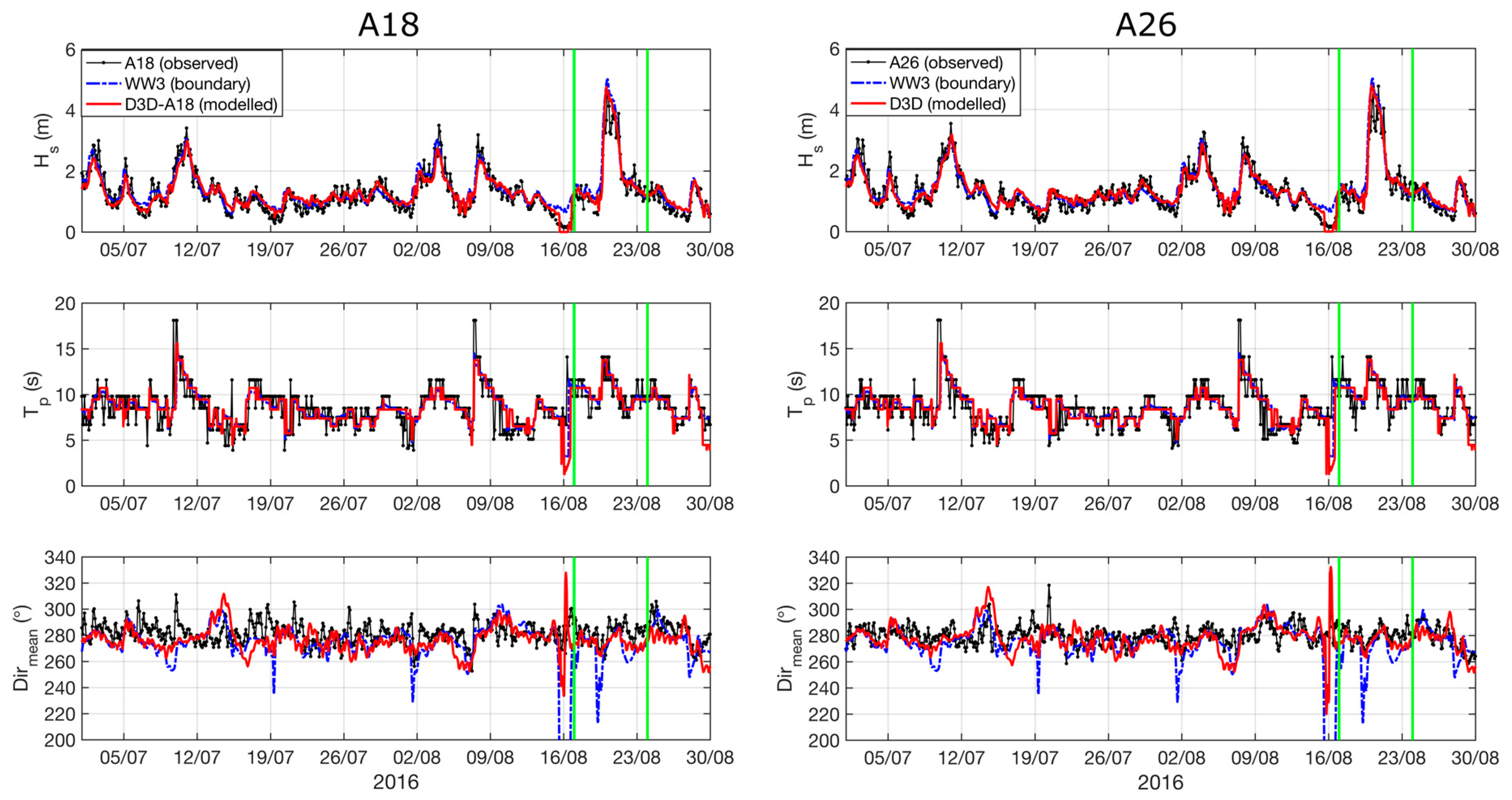
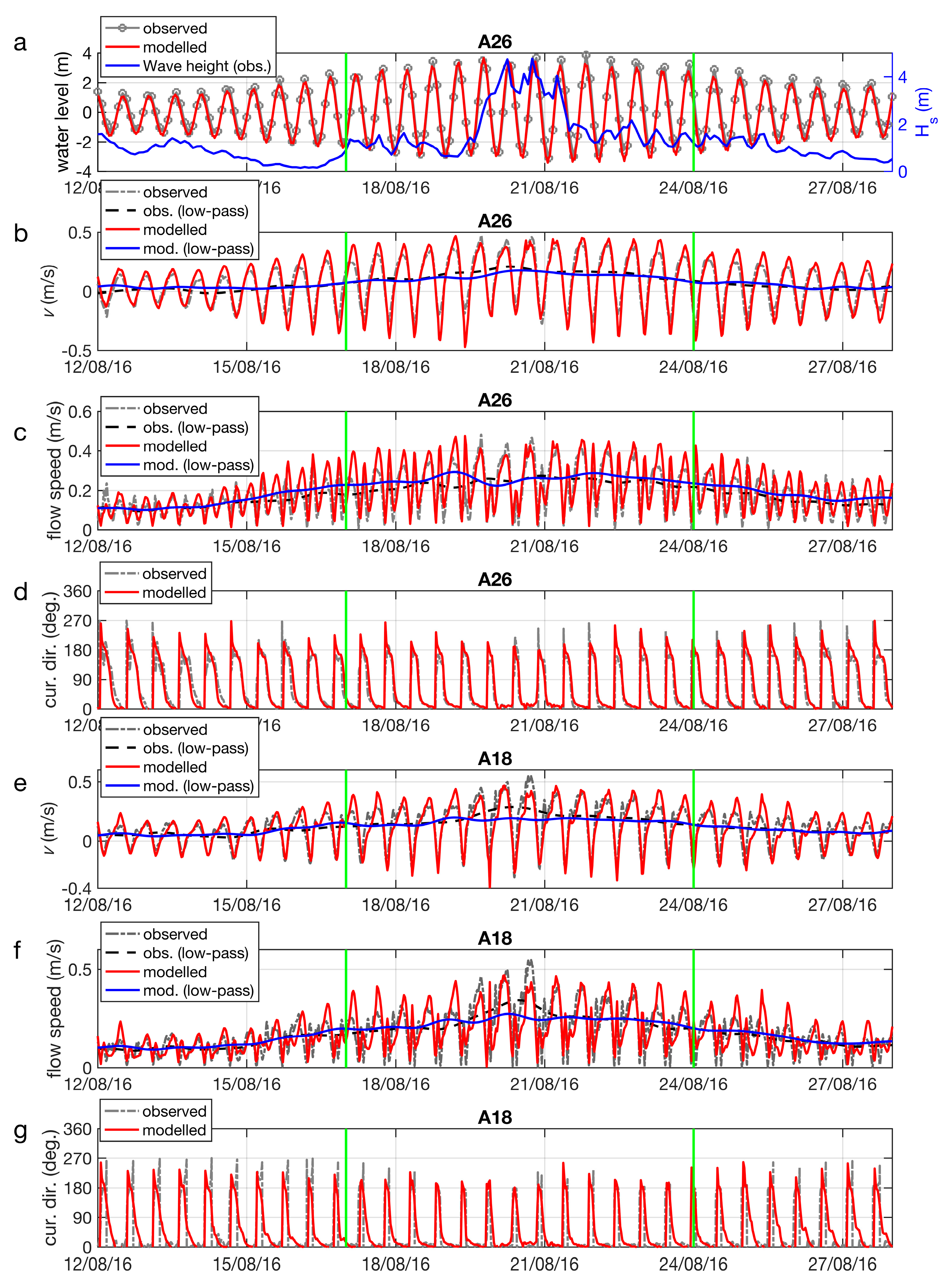
4.1. Model Calibration and Validation
4.1.1. Additional Tests to Assess Sediment Transport Rates
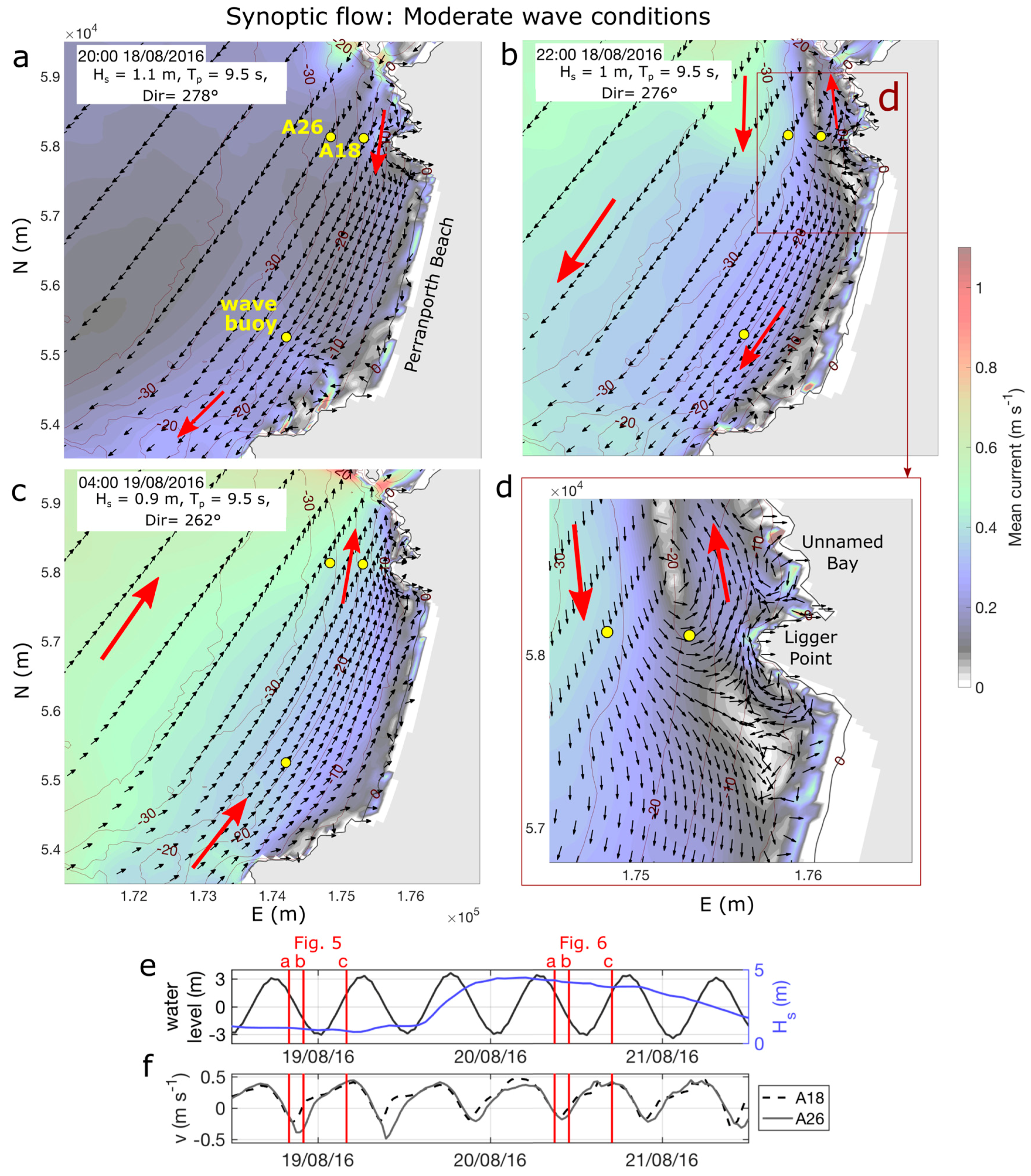
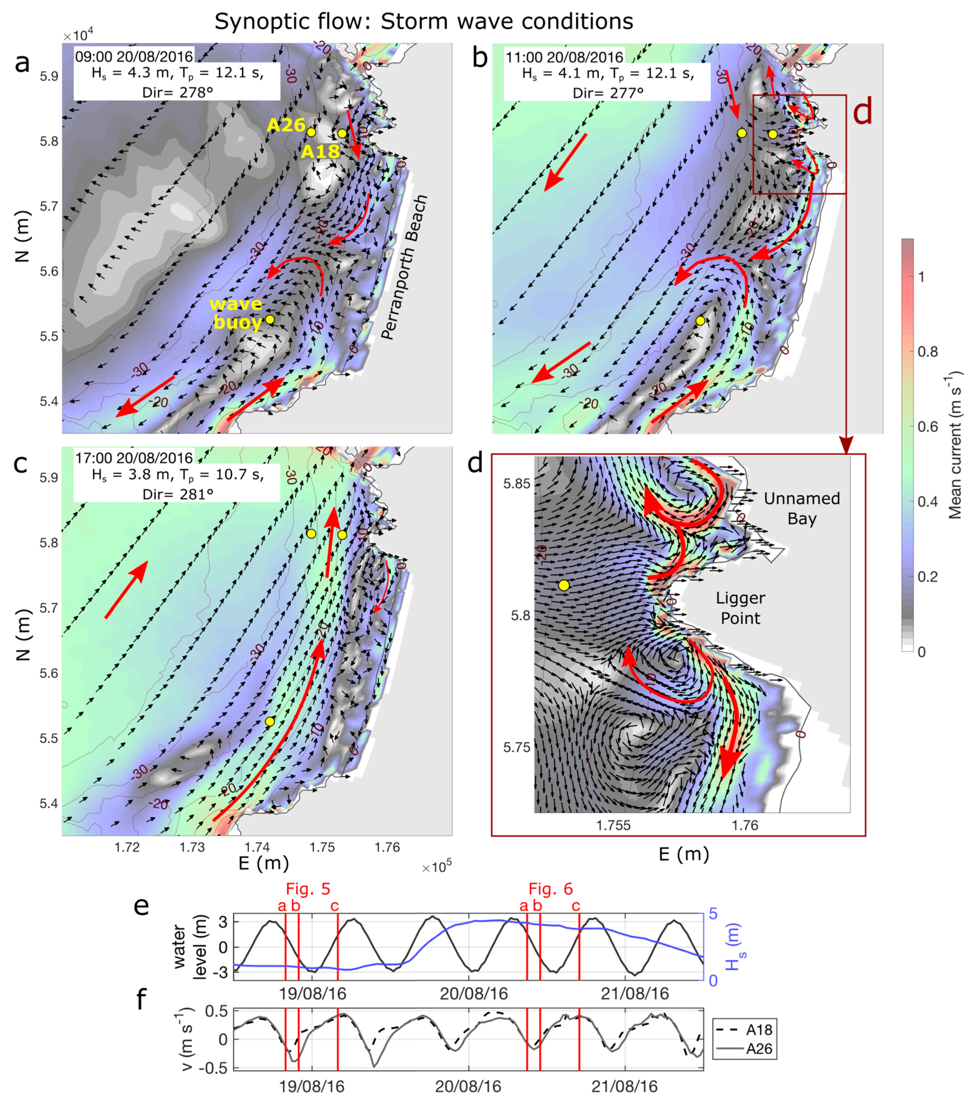
4.2. Synoptic Flow Behaviour
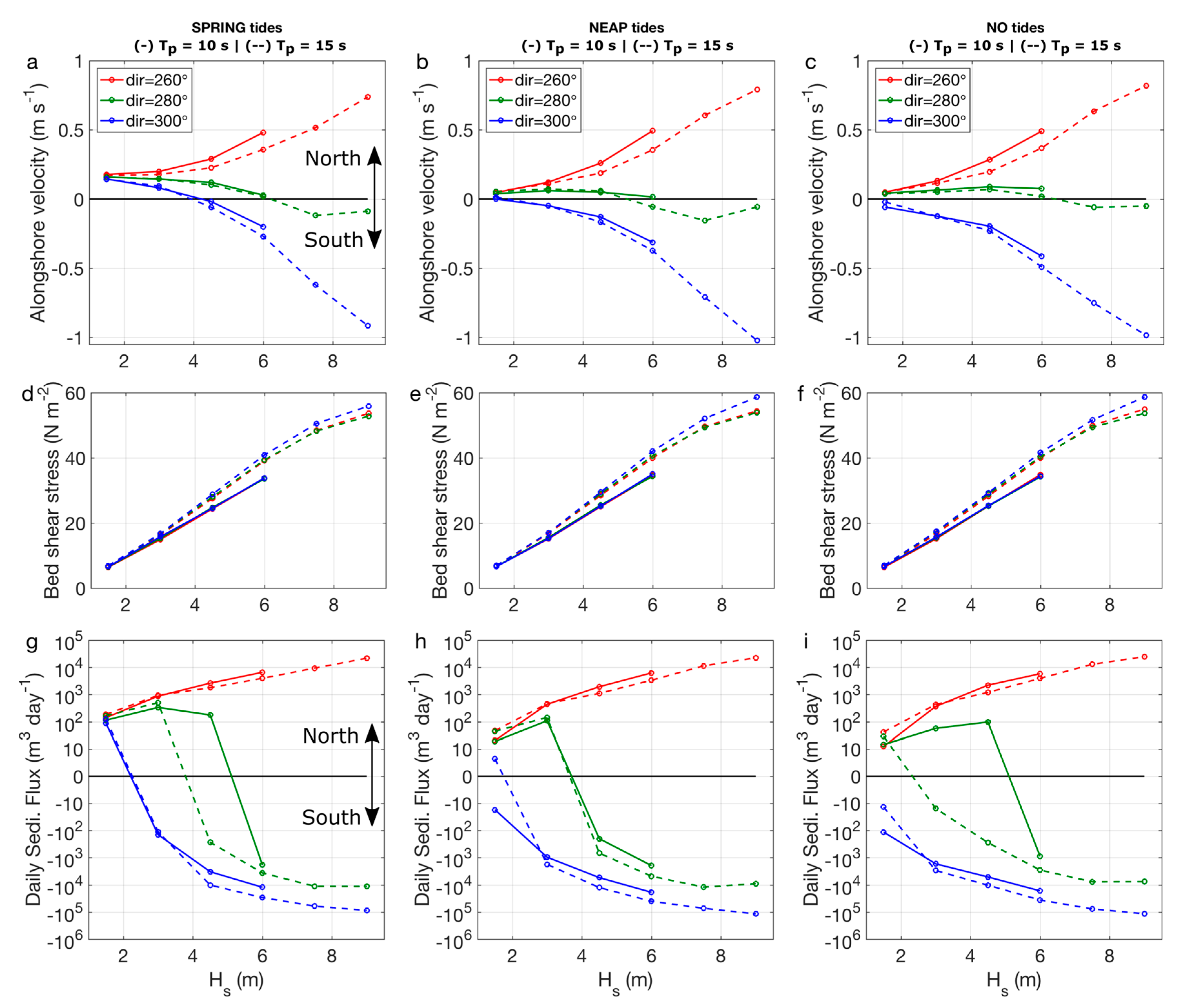
4.3. Wave and Tidal Controls on Flow and Sediment Transport
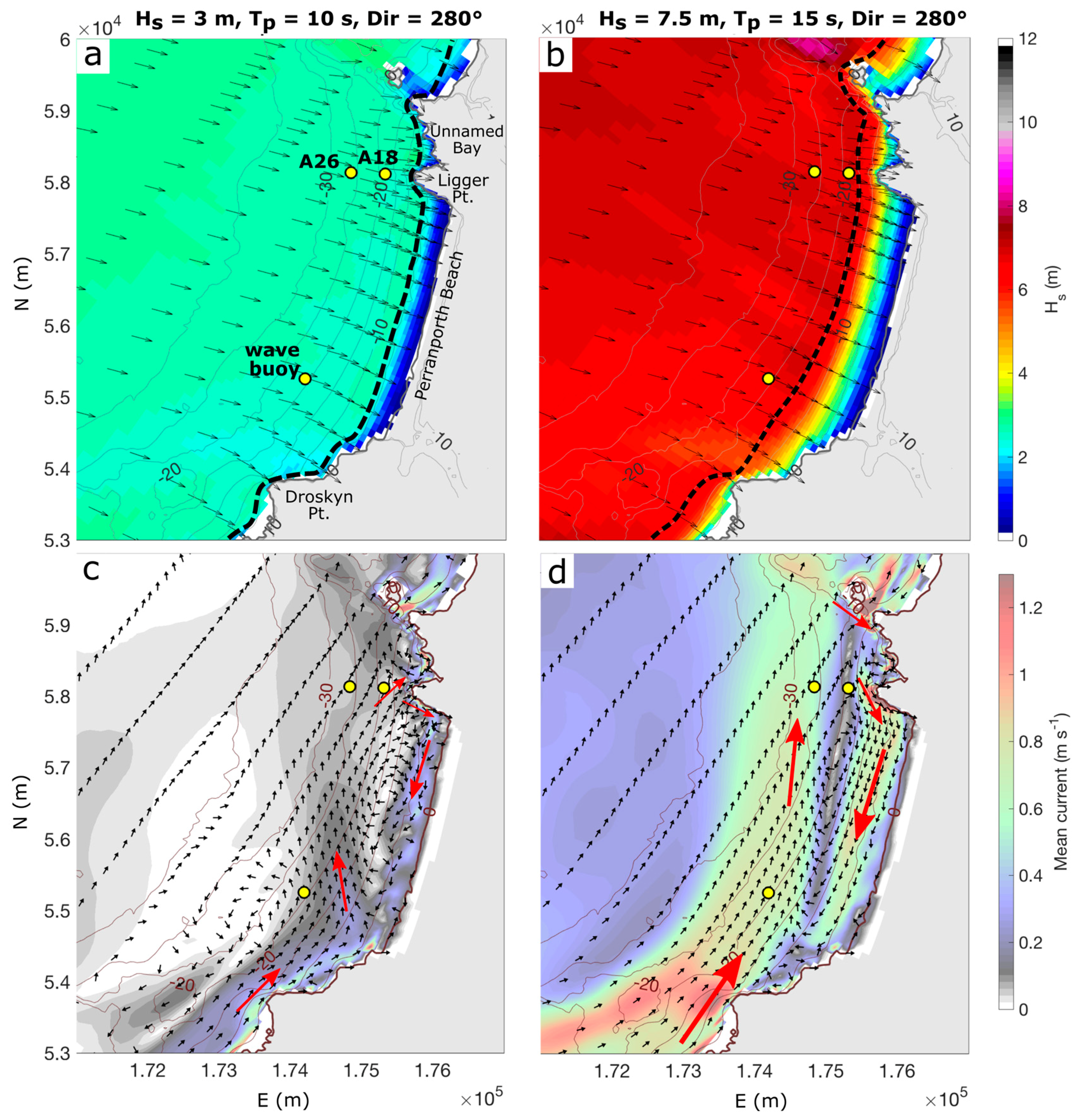
4.4. Synthetic Wave–Tide Scenarios
4.5. Tide-Averaged Embayment-Circulation
5. Discussion
5.1. Modes of Embayment Circulation and Bypassing
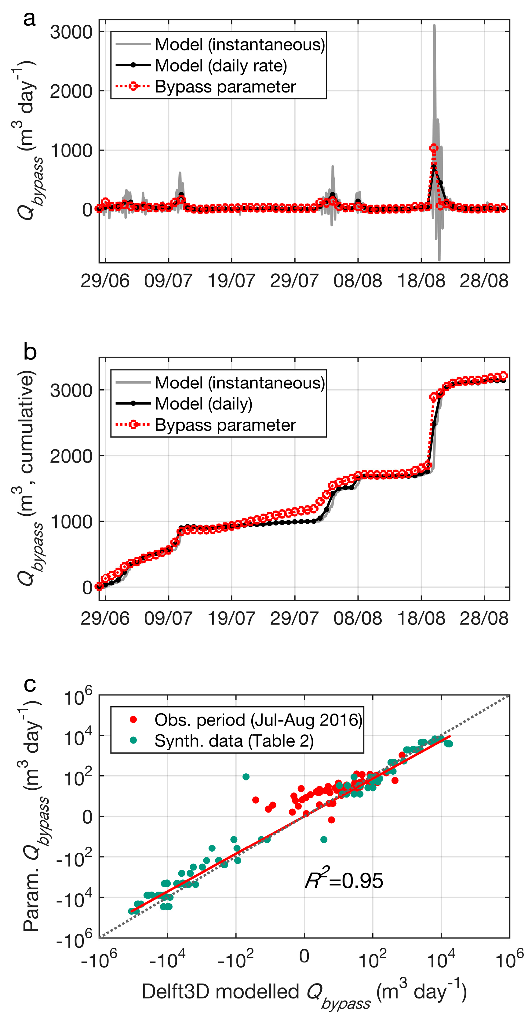
5.2. Daily Headland Bypass Parameter
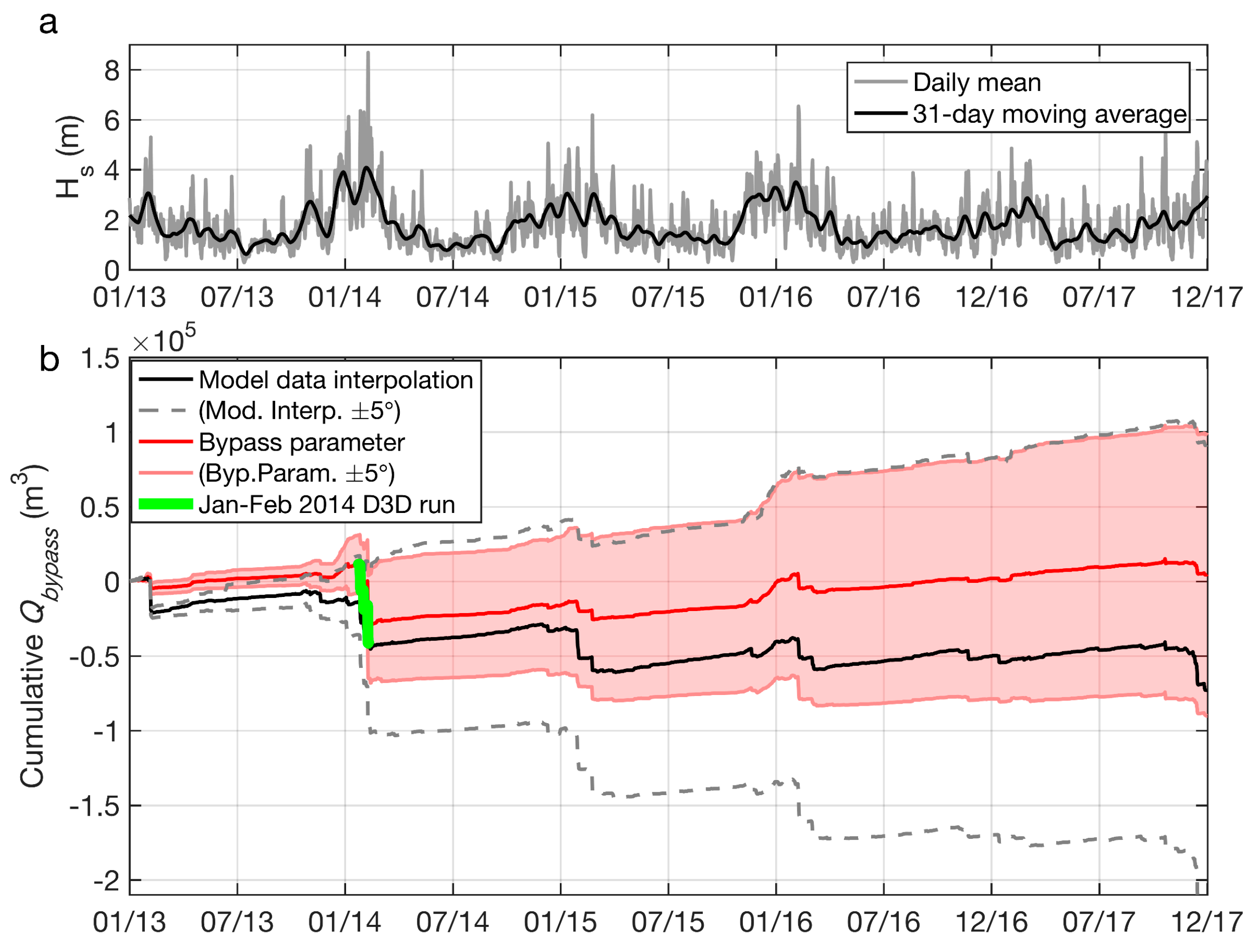
5.3. Prediction of Annual Headland Bypassing Rates
5.4. Implications, Limitations, and Future Research
6. Conclusions
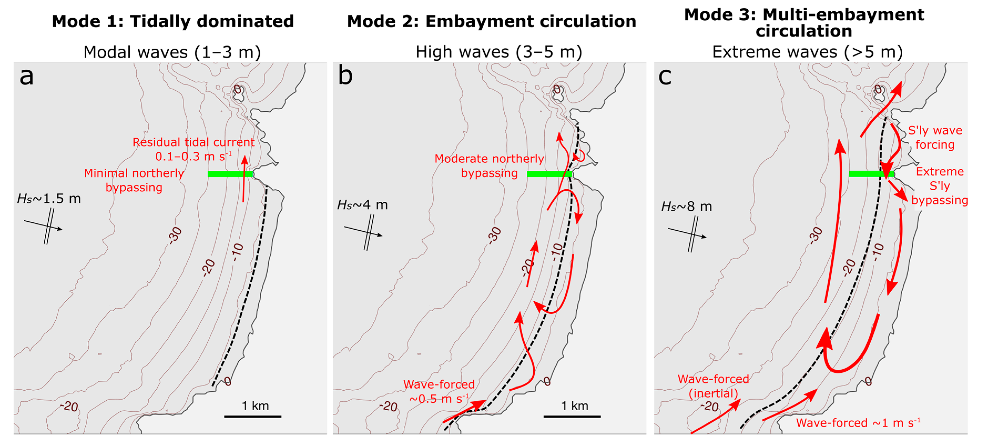
- During low–moderate wave conditions (Hs = 1–3 m), residual tidal currents are the primary control on bypassing direction and magnitude. However, wave-induced shear stress is required to initiate transport. Bypassing rates at the headland of interest are O (0 to +102 m3 day−1).
- For higher waves (Hs = 3–5 m), embayment scale circulation is initiated. For the studied headland, embayment circulation and residual tidal current predominantly acted in the same direction. Bypassing rates are O (103 m3 day−1).
- For extreme waves (Hs > 5 m), waves begin to break beyond the headland, and multi-embayment circulation occurs. For this site, the result was a reversal of the direction of bypassing, overwhelming the forcing of the residual tidal current. Bypassing rates are up to −104 m3 day−1.
Author Contributions
Funding
Acknowledgments
Conflicts of Interest
References
- Davies, J.L. The coastal sediment compartment. Aust. Geogr. Stud. 1974, 12, 139–151. [Google Scholar] [CrossRef]
- Bray, M.J.; Carter, D.J.; Hooke, J.M. Littoral Cell Definition and Budgets for Central Southern England. Source J. Coast. Res. J. Coast. Res. 1995, 11, 381–400. [Google Scholar] [CrossRef]
- Cowell, P.J.; Stive, M.J.F.; Niedoroda, A.W.; De Vriend, H.J.; Swift, D.J.P.; Kaminsky, G.M.; Capobianco, M. The Coastal-Tract (Part 1): A Conceptual Approach to Aggregated Modeling of Low-Order Coastal Change. J. Coast. Res. 2003, 19, 812–827. [Google Scholar] [CrossRef]
- Van Rijn, L.C. Coastal erosion and control. Ocean Coast. Manag. 2011, 54, 867–887. [Google Scholar] [CrossRef]
- Kinsela, M.; Morris, B.; Linklater, M.; Hanslow, D. Second-Pass Assessment of Potential Exposure to Shoreline Change in New South Wales, Australia, Using a Sediment Compartments Framework. J. Mar. Sci. Eng. 2017, 5, 61. [Google Scholar] [CrossRef]
- Castelle, B.; Bujan, S.; Ferreira, S.; Dodet, G. Foredune morphological changes and beach recovery from the extreme 2013/2014 winter at a high-energy sandy coast. Mar. Geol. 2017, 385, 41–55. [Google Scholar] [CrossRef]
- Masselink, G.; Austin, M.; Scott, T.; Poate, T.; Russell, P. Role of wave forcing, storms and NAO in outer bar dynamics on a high-energy, macro-tidal beach. Geomorphology 2014, 226, 76–93. [Google Scholar] [CrossRef]
- Ortiz, A.C.; Ashton, A.D. Exploring shoreface dynamics and a mechanistic explanation for a morphodynamic depth of closure. J. Geophys. Res. Earth Surf. 2016, 121, 442–464. [Google Scholar] [CrossRef]
- Van Rijn, L.C. A simple general expression for longshore transport of sand, gravel and shingle. Coast. Eng. 2014, 90, 23–39. [Google Scholar] [CrossRef]
- Dan, S.; Stive, M.J.F.; Walstra, D.J.R.; Panin, N. Wave climate, coastal sediment budget and shoreline changes for the Danube Delta. Mar. Geol. 2009, 262, 39–49. [Google Scholar] [CrossRef]
- Evans, O.F. The relation of the action of waves and currents on headlands to the control of shore erosion by groins. Proc. Okla. Acad. Sci. 1943, 24, 9–13. [Google Scholar]
- Da Silva, G.V.; Toldo, E.E.; Klein, A.H.D.F.; Short, A.D.; Woodroffe, C.D. Headland sand bypassing—Quantification of net sediment transport in embayed beaches, Santa Catarina Island North Shore, Southern Brazil. Mar. Geol. 2016, 379, 13–27. [Google Scholar] [CrossRef]
- Hsu, J.R.C.; Evans, C. Parabolic Bay Shapes and Applications. Proc. Inst. Civ. Eng. 1989, 87, 557–570. [Google Scholar] [CrossRef]
- Pelnard-Considere, R. Essai de theorie de l’evolution des formes de rivage en plages de sable et de galets. In Les Energies la Mer Compte Rendu Des Quatr. Journees L’hydraulique, Paris 13, 14 15 Juin 1956; Quest. III, Rapp. 1, 74–1-10; Société hydrotechnique de France: Paris, France, 1956. [Google Scholar]
- Larson, M.; Hanson, H.; Kraus, N.C. Analytical solutions of one-line model for shoreline change near coastal structures. J. Waterw. Port Coast. Ocean Eng. 1997, 123, 180–191. [Google Scholar] [CrossRef]
- Scott, T.; Austin, M.; Masselink, G.; Russell, P. Dynamics of rip currents associated with groynes—Field measurements, modelling and implications for beach safety. Coast. Eng. 2016, 107, 53–69. [Google Scholar] [CrossRef]
- Ab Razak, M.S.; Dastgheib, A.; Roelvink, D. Sand bypassing and shoreline evolution near coastal structure, comparing analytical solution and XBeach numerical modelling. J. Coast. Res. 2013, 65, 2083–2088. [Google Scholar] [CrossRef]
- Grant, W.D.; Madsen, O.S. Combined wave and current interaction with a rough bottom. J. Geophys. Res. Ocean. 1979, 84, 1797–1808. [Google Scholar] [CrossRef]
- Olabarrieta, M.; Medina, R.; Castanedo, S. Effects of wave-current interaction on the current profile. Coast. Eng. 2010, 57, 643–655. [Google Scholar] [CrossRef]
- Tambroni, N.; da Silva, J.F.; Duck, R.W.; McLelland, S.J.; Venier, C.; Lanzoni, S. Experimental investigation of the impact of macroalgal mats on the wave and current dynamics. Adv. Water Resour. 2016, 93, 326–335. [Google Scholar] [CrossRef]
- Short, A.D.; Masselink, G. Embayed and structurally controlled embayed beaches. In Handbook of Beach and Shoreface Morphodynamics; Wiley: Hoboken, NJ, USA, 1999; pp. 230–250. [Google Scholar]
- Goodwin, I.D.; Freeman, R.; Blackmore, K. An insight into headland sand bypassing and wave climate variability from shoreface bathymetric change at Byron Bay, New South Wales, Australia. Mar. Geol. 2013, 341, 29–45. [Google Scholar] [CrossRef]
- Castelle, B.; Scott, T.; Brander, R.W.; McCarroll, R.J. Rip current types, circulation and hazard. Earth-Sci. Rev. 2016, 163, 1–21. [Google Scholar] [CrossRef]
- Castelle, B.; Coco, G. The morphodynamics of rip channels on embayed beaches. Cont. Shelf Res. 2012, 43, 10–23. [Google Scholar] [CrossRef]
- Short, A.D. Rip-current type, spacing and persistence, Narrabeen Beach, Australia. Mar. Geol. 1985, 65, 47–71. [Google Scholar] [CrossRef]
- Coutts-Smith, A.J. The Significance of Mega-Rips along an Embayed Coast. Ph.D. Thesis, University of Sydney, Sydney, Australia, 2004. [Google Scholar]
- Loureiro, C.; Ferreira, Ó.; Cooper, J.A.G. Extreme erosion on high-energy embayed beaches: Influence of megarips and storm grouping. Geomorphology 2012, 139–140, 155–171. [Google Scholar] [CrossRef]
- McCarroll, R.J.; Brander, R.W.; Turner, I.L.; Leeuwen, B. Van Shoreface storm morphodynamics and mega-rip evolution at an embayed beach: Bondi Beach, NSW, Australia. Cont. Shelf Res. 2016, 116, 74–88. [Google Scholar] [CrossRef]
- Duarte, J.; Taborda, R.; Ribeiro, M.; Cascalho, J.; Silva, A.; Bosnic, I. Evidences of sediment bypassing at Nazaré headland revealed by a large scale sand tracer experiment. In Proceedings of the 3rd as Jornadas de Engenharia Hidrográica, Lisboa, Portugal, 24–26 June 2014; Volume 2014, pp. 289–292. [Google Scholar]
- Klein, A.H.F.; Ferreira, Ó.; Dias, J.M.A.; Tessler, M.G.; Silveira, L.F.; Benedet, L.; de Menezes, J.T.; de Abreu, J.G.N. Morphodynamics of structurally controlled headland-bay beaches in southeastern Brazil: A review. Coast. Eng. 2010, 57, 98–111. [Google Scholar] [CrossRef]
- George, D.A.; Largier, J.L.; Storlazzi, C.D.; Barnard, P.L. Classification of rocky headlands in California with relevance to littoral cell boundary delineation. Mar. Geol. 2015, 369, 137–152. [Google Scholar] [CrossRef]
- Castelle, B.; Coco, G. Surf zone flushing on embayed beaches. Geophys. Res. Lett. 2013, 40, 2206–2210. [Google Scholar] [CrossRef]
- Ab Razak, M.S.; Dastgheib, A.; Suryadi, F.X.; Roelvink, D. Headland structural impacts on surf zone current circulations. J. Coast. Res. 2014, 70, 65–71. [Google Scholar] [CrossRef]
- Daly, C.J.; Bryan, K.R.; Winter, C. Wave energy distribution and morphological development in and around the shadow zone of an embayed beach. Coast. Eng. 2014, 93, 40–54. [Google Scholar] [CrossRef]
- Daly, C.J.; Bryan, K.R.; Gonzalez, M.R.; Klein, A.H.F.; Winter, C. Effect of selection and sequencing of representative wave conditions on process-based predictions of equilibrium embayed beach morphology Topical Collection on the 7th International Conference on Coastal Dynamics in Arcachon, France, 24–28 June 2013. Ocean Dyn. 2014, 64, 863–877. [Google Scholar] [CrossRef]
- Ashton, A.; Murray, A.B.; Arnault, O. Formation of coastline features by large-scale instabilities induced by high-angle waves. Nature 2001, 414, 296–300. [Google Scholar] [CrossRef] [PubMed]
- Hurst, M.D.; Barkwith, A.; Ellis, M.A.; Thomas, C.W.; Murray, A.B. Exploring the sensitivities of crenulate bay shorelines to wave climates using a new vector-based one-line model. J. Geophys. Res. F Earth Surf. 2015, 120, 2586–2608. [Google Scholar] [CrossRef]
- George, D.A.; Largier, J.L.; Pasternack, G.B.; Erikson, L.H.; Storlazzi, C.D.; Barnard, P. Modeling Sediment Bypassing around Rocky Headlands. In AGU Fall Meeting Abstracts; American Geophysical Union: Washington, DC, USA, 2016. [Google Scholar]
- Da Silva, G.V.; Toldo, E.E.; Klein, A.H.F.; Short, A.D.; Tomlinson, R.; Strauss, D. A comparison between natural and artificial headland sand bypassing in Santa Catarina and the Gold Coast. In Proceedings of the Australasian Coasts & Ports 2017: Working with Nature, Cairns Convention Centre, Cairns, Australia, 21–23 June 2017; p. 1111. [Google Scholar]
- Da Silva, G.V.; Toldo, E.E., Jr.; Klein, A.H.D.F.; Short, A.D. The influence of wave-, wind-and tide-forced currents on headland sand bypassing–Study case: Santa Catarina Island north shore, Brazil. Geomorphology 2018, 312, 1–11. [Google Scholar] [CrossRef]
- Valiente, N.G.; Masselink, G.; Scott, T.; Conley, D. Depth of Closure Along an Embayed, Macro-Tidal and Exposed Coast: A Multi-Criteria Approach. Coast. Dyn. 2017, Paper 185. 1211–1222. [Google Scholar]
- Scott, T.; Masselink, G.; O’Hare, T.; Saulter, A.; Poate, T.; Russell, P.; Davidson, M.; Conley, D. The extreme 2013/2014 winter storms: Beach recovery along the southwest coast of England. Mar. Geol. 2016, 382, 224–241. [Google Scholar] [CrossRef]
- Masselink, G.; Scott, T.; Poate, T.; Russell, P.; Davidson, M.; Conley, D. The extreme 2013/2014 winter storms: Hydrodynamic forcing and coastal response along the southwest coast of England. Earth Surf. Process. Landf. 2016, 41, 378–391. [Google Scholar] [CrossRef]
- Prodger, S.; Russell, P.; Davidson, M.; Miles, J.; Scott, T. Understanding and predicting the temporal variability of sediment grain size characteristics on high-energy beaches. Mar. Geol. 2016, 376, 109–117. [Google Scholar] [CrossRef]
- Masselink, G.; Short, A.D. The effect of tide range on beach morphodynamics and morphology: A conceptual beach model. J. Coast. Res. 1993, 9, 785–800. [Google Scholar]
- Scott, T.; Masselink, G.; Russell, P. Morphodynamic characteristics and classification of beaches in England and Wales. Mar. Geol. 2011, 286, 1–20. [Google Scholar] [CrossRef]
- Valiente, N.G.; Masselink, G.; Scott, T.; Conley, D.; McCarroll, R.J. Evaluation of the role of waves and tides on depth of closure and potential for headland bypassing. Mar. Geol. 2018. under review. [Google Scholar]
- Lesser, G.R.; Roelvink, J.A.; van Kester, J.A.T.M.; Stelling, G.S. Development and validation of a three-dimensional morphological model. Coast. Eng. 2004, 51, 883–915. [Google Scholar] [CrossRef]
- Luijendijk, A.P.; Ranasinghe, R.; de Schipper, M.A.; Huisman, B.A.; Swinkels, C.M.; Walstra, D.J.R.; Stive, M.J.F. The initial morphological response of the Sand Engine: A process-based modelling study. Coast. Eng. 2017, 119, 1–14. [Google Scholar] [CrossRef]
- Booij, N.; Ris, R.C.; Holthuijsen, L.H. A third-generation wave model for coastal regions: 1. Model description and validation. J. Geophys. Res. 1999, 104, 7649–7666. [Google Scholar] [CrossRef]
- Tolman, H.L. A Third-Generation Model for Wind Waves on Slowly Varying, Unsteady, and Inhomogeneous Depths and Currents. J. Phys. Oceanogr. 1991, 21, 782–797. [Google Scholar] [CrossRef]
- Hsu, Y.L.; Dykes, J.D.; Allard, R.A.; Kaihatu, J.M. Evaluation of Delft3D Performance in Nearshore Flows; Naval Research Laboratory: Washington, DC, USA, 2006. [Google Scholar]
- Hydraulics, D. Delft3D-FLOW User Manual; Deltares: Delft, The Netherlands, 2006. [Google Scholar]
- O’Dea, E.J.; Arnold, A.K.; Edwards, K.P.; Furner, R.; Hyder, P.; Martin, M.J.; Siddorn, J.R.; Storkey, D.; While, J.; Holt, J.T.; et al. An operational ocean forecast system incorporating NEMO and SST data assimilation for the tidally driven European North-West shelf. J. Oper. Oceanogr. 2012, 5, 3–17. [Google Scholar] [CrossRef]
- Fredsøe, J. Turbulent boundary layer in wave-current motion. J. Hydraul. Eng. 1984, 110, 1103–1120. [Google Scholar] [CrossRef]
- Grunnet, N.M.; Walstra, D.J.R.; Ruessink, B.G. Process-based modelling of a shoreface nourishment. Coast. Eng. 2004, 51, 581–607. [Google Scholar] [CrossRef]
- Van Rijn, L.C. A unified view of sediment transport by currents and waves. II: Suspended transport. J. Hydr. Eng. 2006, 133, 649–667. [Google Scholar] [CrossRef]
- Davidson, M.A.; Lewis, R.P.; Turner, I.L. Forecasting seasonal to multi-year shoreline change. Coast. Eng. 2010, 57, 620–629. [Google Scholar] [CrossRef]
- Van Rijn, L.C.; Wasltra, D.J.R.; Grasmeijer, B.; Sutherland, J.; Pan, S.; Sierra, J.P. The predictability of cross-shore bed evolution of sandy beaches at the time scale of storms and seasons using process-based profile models. Coast. Eng. 2003, 47, 295–327. [Google Scholar] [CrossRef]
- Van Rijn, L.C.; Grasmeijer, B.T.; Ruessink, B.G. Measurement Errors of Instruments for Velocity, Wave Height, Sand Concentration and Bed Levels in Field Conditions; Hydraulic Engineering Reports; Deltares: Delft, The Netherlands, 2000. [Google Scholar]
- Masselink, G.; Castelle, B.; Scott, T.; Dodet, G.; Suanez, S.; Jackson, D.; Floc’h, F. Extreme wave activity during 2013/2014 winter and morphological impacts along the Atlantic coast of Europe. Geophys. Res. Lett. 2016, 43, 2135–2143. [Google Scholar] [CrossRef]
- Long, J.W.; Özkan-Haller, H.T. Offshore controls on nearshore rip currents. J. Geophys. Res. Ocean. 2005, 110, 1–21. [Google Scholar] [CrossRef]
- McCarroll, R.J.; Brander, R.W.; Turner, I.L.; Power, H.E.; Mortlock, T.R. Lagrangian observations of circulation on an embayed beach with headland rip currents. Mar. Geol. 2014, 355, 173–188. [Google Scholar] [CrossRef]


| Module | Parameter | Value/Setting | Comment |
|---|---|---|---|
| Hydrodynamics | Eddy diffusivity | 0.1 (m2 s−1) | As per [49]. |
| Horizontal eddy viscosity | 1.0 (m2 s−1) | As per [49]. | |
| Roughness | Chezy (55 m1/2 s−1) | Varying value tested but found to be ineffective. | |
| Waves | Roller model | ON | Reproduced observed currents during storm conditions. Default settings used. |
| Transport | Formulation | Van Rijn (2007b) | ‘TRANSPOOR2004’, as per [49,56]. |
| D50 | 330 microns | As per [44]. | |
| Transport multipliers | Sus (1.4), Bed (0.8), SusW (0.3), BedW (0.3) | Suspended and bed transport multipliers for currents (Sus, Bed) and waves (SusW, BedW). As per [56]. | |
| Morphology | ThetSD | 1.0 | Factor for erosion of adjacent dry cells, as per [49]. |
| MORFAC | 1.0 | Morphological acceleration disabled. |
| Variable | Values |
|---|---|
| Wave | |
| Significant wave height | 1.5 m, 3 m, 4.5 m, 6 m, 7.5 m, 9 m. |
| Peak period | 10 s, 15 s. |
| Direction (relative to shore normal) | 20° S, 0°, 20° N. |
| Tide | Springs, Neaps, No tide. |
| - | - | - | Calibration (1 Week) | Validation (2 Months) | |||||
|---|---|---|---|---|---|---|---|---|---|
| Model | - | Location | RMSE | R2 | BSS | RMSE | R2 | BSS | |
| WAVE | Significant wave height (m) | A26 | 0.39 | 0.89 | 0.90 | 0.25 | 0.85 | 0.91 | |
| - | A18 | 0.36 | 0.91 | 0.92 | 0.25 | 0.85 | 0.91 | ||
| - | Buoy | 0.35 | 0.92 | 0.92 | 0.24 | 0.85 | 0.91 | ||
| - | Peak period (s) | A26 | 1.20 | 0.48 | 0.79 | 1.65 | 0.42 | 0.60 | |
| - | - | A18 | 1.09 | 0.52 | 0.80 | 1.58 | 0.45 | 0.62 | |
| - | - | Buoy | 1.18 | 0.57 | 0.81 | 1.83 | 0.40 | 0.58 | |
| - | Mean direction (deg.) | A26 | 7.2 | 0.19 | 0.42 | 8.6 | 0.18 | 0.33 | |
| - | A18 | 10.4 | 0.10 | 0.10 | 10.6 | 0.05 | 0.11 | ||
| FLOW | Water level | A26 | 0.39 | 0.97 | 0.97 | 0.28 | 0.98 | 0.98 | |
| - | (m) | A18 | 0.42 | 0.97 | 0.96 | 0.28 | 0.98 | 0.98 | |
| - | Flow speed | A26 | 0.07 | 0.67 | 0.72 | 0.06 | 0.69 | 0.72 | |
| - | (m/s) | A18 | 0.08 | 0.55 | 0.67 | 0.06 | 0.55 | 0.66 | |
| - | Residual flow | A26 | 0.03 | 0.14 | 0.15 | 0.02 | 0.91 | 0.90 | |
| - | speed (m s−1) | A18 | 0.03 | 0.68 | 0.76 | 0.02 | 0.87 | 0.93 | |
| - | Flow direction | A26 | 29.9 | 0.88 | 0.84 | 36.1 | 0.81 | 0.77 | |
| - | (deg.) | A18 | 38.9 | 0.74 | 0.72 | 47.6 | 0.69 | 0.66 | |
| Forcing Scenario | DAILY Sediment Bypass Rates | Forcing Controls |
|---|---|---|
| Flat conditions, any tide. | ~0 m3 day−1 | Wave-stirring required for transport to initiate. Tidal current alone produces negligible flux (Figure 7, red line). |
| Modal waves, neap tides. | ~101 m3 day−1 | Combination of weak residual tidal flow (northward) and offshore wave direction, (Figure 8h). |
| Modal waves (1–3 m), spring tides. | ~102 m3 day−1 | In direction of residual tidal flow (northward), (Figure 8g). |
| High waves (3–5 m), any tide. | 102–103 m3 day−1 | Transport controlled by wave direction and residual tidal current, biased toward the north (Figure 8g,h; Figure 10-left column). |
| Extreme waves (>5 m), any tide. | 103–104 m3 day−1 | Multi-embayment circulation develops, transport biased toward the south (Figure 8g,h; Figure 10-right column). |
| Time Period | Sediment Bypass Rates | Comment |
|---|---|---|
| Spring–Autumn | ~ 104 m3 over 8–9 months | Gradual, persistent northward flux. |
| Winter | (0 to −5) × 104 m3 over 3–4 months | Episodic, rapid southward flux with large storms. |
| Annual rate | (+1 to −3) × 104 m3 year−1 | Net transport direction varies, depending on winter wave energy. |
© 2018 by the authors. Licensee MDPI, Basel, Switzerland. This article is an open access article distributed under the terms and conditions of the Creative Commons Attribution (CC BY) license (http://creativecommons.org/licenses/by/4.0/).
Share and Cite
McCarroll, R.J.; Masselink, G.; Valiente, N.G.; Scott, T.; King, E.V.; Conley, D. Wave and Tidal Controls on Embayment Circulation and Headland Bypassing for an Exposed, Macrotidal Site. J. Mar. Sci. Eng. 2018, 6, 94. https://doi.org/10.3390/jmse6030094
McCarroll RJ, Masselink G, Valiente NG, Scott T, King EV, Conley D. Wave and Tidal Controls on Embayment Circulation and Headland Bypassing for an Exposed, Macrotidal Site. Journal of Marine Science and Engineering. 2018; 6(3):94. https://doi.org/10.3390/jmse6030094
Chicago/Turabian StyleMcCarroll, R. Jak, Gerd Masselink, Nieves G. Valiente, Tim Scott, Erin V. King, and Daniel Conley. 2018. "Wave and Tidal Controls on Embayment Circulation and Headland Bypassing for an Exposed, Macrotidal Site" Journal of Marine Science and Engineering 6, no. 3: 94. https://doi.org/10.3390/jmse6030094
APA StyleMcCarroll, R. J., Masselink, G., Valiente, N. G., Scott, T., King, E. V., & Conley, D. (2018). Wave and Tidal Controls on Embayment Circulation and Headland Bypassing for an Exposed, Macrotidal Site. Journal of Marine Science and Engineering, 6(3), 94. https://doi.org/10.3390/jmse6030094