Free Surface Reconstruction for Phase Accurate Irregular Wave Generation

Abstract

The experimental wave paddle signal is unknown to the numerical modellers in many cases. This makes it quite challenging to numerically reproduce the time history of free surface elevation for irregular waves. In the present work, a numerical investigation is performed using a computational fluid dynamics (CFD) based model to validate and investigate a non-iterative free surface reconstruction technique for irregular waves. In the current approach, the free surface is reconstructed by spectrally composing the irregular wave train as a summation of the harmonic components coupled with the Dirichlet inlet boundary condition. The verification is performed by comparing the numerically reconstructed free surface elevation with theoretical input waves. The applicability of the present approach to generate irregular waves by reconstructing the free surface is investigated for different coastal and marine engineering problems. A numerical analysis is performed to validate the free surface reconstruction approach to generate breaking irregular waves over a submerged bar. The wave amplitudes, wave frequencies and wave phases are modelled with good accuracy in the time-domain during the higher-order energy transfers and complex processes like wave shoaling, wave breaking and wave decomposition. The present approach to generate irregular waves is also employed to model steep irregular waves in deep water. The free surface reconstruction method is able to simulate the irregular free surface profiles in deep water with low root mean square errors and high correlation coefficients. Furthermore, the irregular wave forces on a monopile are investigated in the time-domain. The amplitudes and phases of the force signal under irregular waves generated by using the current technique are modelled accurately in the time-domain. The proposed approach to numerically reproduce the free surface elevation in the time-domain provides promising and accurate results for all the benchmark cases.

1. Introduction

The real sea state is highly random and stochastic in nature. The most common external force responsible for generating the ocean surface waves is wind. The frequency range associated with wind is quite wide which causes a broad range of wavelengths, amplitudes, phases and periods in the ocean surface. This makes the study of the real sea state quite complex. The frequency-domain investigation provides information to understand the wave energy distribution at various frequencies. The time-domain analysis is equally important because parameters such as surface elevation, orbital velocities, instantaneous response forces, and higher-order effects can be computed from the time-series of a given quantity. The auto- and cross-correlation functions are determined from the measured wave records [1]. These functions can be further used to perform the harmonic analysis of the time-series data. The recent developments in the efficiency of computational resources and development of several numerical techniques have led to an increased application of numerical models in solving coastal and marine wave problems. Numerical models have been found to be reliable, cost effective and time saving tools [2,3,4,5]. However, a good validation with experiments is required in order to employ the numerical model for real-world applications with confidence. In the absence of experimental wavemaker kinematics information, numerical models usually employ random phases to generate irregular wave groups or focused wave groups, which then makes the wave phases in numerical signals to differ from the experimental signals. The calibration of the numerical waves in frequency-domain is the only solution in such conditions. Generally, the numerical models require experimental wavemaker input for reproducing the irregular wave signals in the time-domain. The wavemaker kinematics information is not available to numerical modellers in many cases. The phase and amplitude information of each individual wave component is required in order to reproduce the experimental free surface elevation time-series in the numerical models. Some researchers have made notable efforts in the past to investigate the free surface elevation in the time-domain using the stream functions, the wavelet approach and Fast Fourier Transform (FFT) technique [6,7,8].

Dean [9] suggested an analytical stream function method to represent the nonlinear ocean waves in the time-domain from either a measured wave form or specified gross wave characteristics (wave height, wave period, water depth). Tromans et al. [10] developed a new model to predict the kinematics of large ocean waves. They proposed a linear broad-banded wave theory in which the component wavelets are assigned amplitudes and phases. The wavelet approach was further utilised to post-process the time series and to detect a complex variability in both time and frequency domains for various applications including non-stationary deep water waves, waves breaking at the tropical coral reefs and mechanically generated waves in the wave flume [11]. Many studies have applied spectral decomposition methods in both space and time domains for resolving the large scale disturbances to their individual wave components [12,13,14,15]. They used the assumption of ergodic processes for the wind waves and performed the spectral, cross-spectral and bi-spectral analyses [16]. The spectral decomposition method for harmonic components can provide useful information about individual wave amplitudes, wave phases and wave frequencies for irregular waves. The computed wave parameters can be further utilized to reconstruct the irregular ocean wave surface with an assumption that the irregular sea state can be represented by the superposition of individual regular wave components [17]. This approach to replicate the experimental free surface elevation without any information about the experimental wavemaker inputs could be of great interest for the numerical modelling.

Many researchers in the past have applied CFD (Computational Fluid Dynamics) based numerical models to study different types of non-breaking and breaking waves [18,19,20,21,22]. The CFD models have been validated for irregular waves generated using the random phases in the frequency-domain [23,24,25,26]. Few researchers have made attempts to reconstruct the experimental non-breaking and breaking irregular waves in the time-domain without experimental wavemaker inputs. Panchang et al. [27,28] and Bredmose and Jacobsen [29], Bredmose et al. [30] applied the free surface reconstruction approach for different applications including the investigation of nonlinear and breaking wave loads on offshore wind turbine substructures with regular, irregular and focused wave groups and ideal flip-through impact on the vertical face of breakwater or seawall, respectively. They used an iterative method to reconstruct the target wave field by employing the linear approach initially given by Goda and Suzuki [31] and Mansard and Funke [32] for the reflection analysis. The complex wave amplitudes for the incident and reflected wave components were computed at different frequencies by using the linear least squares method. The computed linear wave field was imposed as a boundary condition. In the next step, an iterative ad hoc procedure was performed until the computed wave field matched the target wave field within a first-order of accuracy. They compared the reconstructed numerical and experimental results for free surface and wave forces in the time-domain. The numerical results with their wave reconstruction technique illustrated promising results. However, some differences in the peak wave crests and wave phases were observed in cases of steep irregular and focused waves. Buldakov et al. [33] utilised the harmonics separation technique for the iterative focusing of a linearised amplitude spectrum rather than to a full nonlinear spectrum for focused wave groups.

The objective of the present work is to investigate the applicability of the proposed non-iterative free surface reconstruction approach for different coastal and marine engineering nonlinear wave problems. The numerical analysis is performed with the open-source hydrodynamics model REEF3D [34]. The numerical model has been successfully used to study various coastal and marine engineering problems [22,24,35,36,37]. The present approach to reconstruct the irregular free surface elevation is based on the coupling of the Dirichlet inlet boundary condition with the irregular wave characteristics. First, the wave amplitudes, wave phases and frequencies of the individual wave components of the target irregular wave train are computed. Next, the irregular waves are generated using the linear superposition concept. The proposed methodology to numerically reconstruct the experimental free surface signal at any location in the time-domain is non-iterative. The current approach requires the information of the experimental free surface elevation signal at only one wave gauge location. The sampling interval is chosen sufficiently small so that most of the wave components are correctly captured in the time-domain. The frequency range to discretize the wave spectrum is selected such that the harmonic components in the higher-frequency range are also captured and the wave nonlinearity can be represented. The generated phase accurate irregular wave train then propagates in the CFD based numerical wave tank simulating the wave transformation and wave propagation including the higher-order affects like wave shoaling, wave breaking and wave decomposition and associated super- and sub-harmonics. The non-iterative nature of the present approach makes it more time-efficient and quite practical from the numerical modelling point of view.

At first, a grid refinement study is performed for two offshore wave steepness cases in the numerical wave tank with a constant water depth in order to test and verify the irregular wave generation and propagation with the waves generated by using the free surface reconstruction technique (Section 3.1). Furthermore, breaking irregular waves over a submerged bar are modelled. The reconstructed numerical wave signal at different positions is compared with the experimental wave signal in the time-domain [38]. The numerical waves generated using the free surface reconstruction method are able to simulate the complex wave transformation process including wave shoaling, wave breaking and wave decomposition with a good accuracy, which indicates the capability of this technique to replicate the experimental waves in the time-domain without experimental wavemaker input (Section 3.2). Section 3.3 presents the study of the free surface reconstruction method to model the irregular waves with large spectral steepness in deep water. The numerical and experimental free surface signals are compared for this case [39]. Section 3.4 presents the applicability of the wave reconstruction technique to model irregular wave forces. The numerical free surface and force signals are compared with the experiments by Pákozdi et al. [40] in the time-domain and the resulting errors are computed. The capability of the present free surface reconstruction approach to model higher-order components with accurate phases and amplitudes in the free surface elevation signals and force signals is highlighted in this section by an investigation in both time and frequency domains.

2. CFD Model

2.1. Overview of the Numerical Schemes

The open-source hydrodynamics model REEF3D is based on the governing equations of fluid dynamics: continuity equation and the Reynolds Averaged Navier–Stokes equations (RANS) with the assumption of an incompressible fluid given as:

$$\frac{\partial u_i}{\partial x_i}=0,$$

(1)

$$\frac{\partial u_i}{\partial t}+u_j\frac{\partial u_i}{\partial x_j}=-\frac{1}{\rho }\frac{\partial p}{\partial x_i}+\frac{\partial }{\partial x_j}\left[(\nu +{\nu }_t)\left(\frac{\partial u_i}{\partial x_j}+\frac{\partial u_j}{\partial x_i}\right)\right]+g_i,$$

(2)

where u is the velocity averaged over time t, $\rho$ is the fluid density, p is the pressure, $\nu$ is the kinematic viscosity, ${\nu }_t$ is the eddy viscosity, i and j denote the indices in the x- and y-direction, respectively and $g_i$ is the acceleration due to gravity.

The numerical model uses a fifth-order finite difference Weighted Essentially Non-Oscillatory (WENO) scheme in multi-space dimensions for the spatial discretization [41]. The third-order TVD Runge–Kutta scheme is used for the time discretization [42]. An adaptive time stepping scheme is used in the numerical model [43]. The present study uses the $k-\omega$ model used to calculate the eddy-viscosity by solving for the turbulent kinetic energy k and the specific turbulent dissipation $\omega$ [44]:

$$\frac{\partial k}{\partial t}+u_j\frac{\partial k}{\partial x_j}=\frac{\partial }{\partial x_j}\left[\left(\nu +\frac{{\nu }_t}{{\sigma }_k}\right)\frac{\partial k}{\partial x_j}\right]+P_k-{\beta }_{k}k\omega ,$$

(3)

$$\frac{\partial \omega }{\partial t}+u_j\frac{\partial \omega }{\partial x_j}=\frac{\partial }{\partial x_j}\left[\left(\nu +\frac{{\nu }_t}{{\sigma }_{\omega }}\right)\frac{\partial \omega }{\partial x_j}\right]+\frac{\omega }{k}\alpha P_k-\beta {\omega }^2,$$

(4)

where $P_k$ is the turbulent production rate and is defined as follows:

$$P_k={\nu }_t\frac{\partial u_i}{\partial x_j}[\frac{\partial u_i}{\partial x_j}+\frac{\partial u_j}{\partial x_i}].$$

(5)

The other closure coefficients are $\alpha =\frac{5}{9}$, ${\beta }_k=\frac{9}{100}$, $\beta =\frac{3}{40}$, ${\sigma }_{\omega }=2$, ${\sigma }_k=2$. The over-production of the turbulence in highly strained flow associated with the oscillatory fluid motion under waves outside the boundary layer is prevented by limiting the eddy-viscosity [45] as follows:

$${\nu }_t=\min (\frac{k}{\omega },\sqrt{\frac{2}{3}}\frac{k}{S}),$$

(6)

where S is the mean rate of strain.

The level set method is used to capture the free surface [46]. The level set function defines the free surface as:

$$\varphi (\overrightarrow{x},t)\left\{\begin{array}{cc}>0,\hfill & if\overrightarrow{x}isinphase1,\hfill \\ =0,\hfill & if\overrightarrow{x}isattheinterface,\hfill \\ <0,\hfill & if\overrightarrow{x}isinphase2.\hfill \end{array}\right.$$

(7)

A three-dimensional ghost cell immersed boundary method (GCIBM) [47] is adapted to model complex geometries. Parallel computation is employed in the numerical model which is based on the domain decomposition method and MPI (message passing interface). The detailed information about the numerical model can be obtained in [34] and Bihs and Kamath [48]. In the present work, the waves are generated by employing the Dirichlet inlet boundary condition, and they are dissipated with the active wave absorption method at the outlet boundary [49]. This combination of the wave generation and absorption methods allows the use of relatively shorter numerical domains.

For the wave force calculation, the computed pressure and normal viscous stresses around the cylinder is integrated over the surface $\Gamma$ for calculating the force, which can be given as:

$$F={\int }_{\Gamma }(-np+n.\tau )d\Gamma ,$$

(8)

where p represents the pressure and $\tau$ is the normal component of the stress tensor. The numerical model has been used in the past for a wide range of marine applications such as wave-structure interaction [50,51], breaking wave forces [35], floating body dynamics [48], sloshing [52], irregular wave analysis [24,37,53] and sediment transport [54].

2.2. Free Surface Reconstruction

The present approach to reconstruct the free surface elevation is based on the spectral decomposition technique for the harmonic components. The Fourier analysis differentiates the variability of the time–series into components at the frequencies of each harmonic and approximates a function as a summation of the sine and cosine terms. The irregular wave signal in experimental wave flumes measured at a target location consists of incident and reflected signals:

$$x(t)=x_{in}(t)+x_r(t),$$

(9)

where $x_{in}(t)$ is the incident wave signal and $x_r(t)$ is the reflected wave signal.

Furthermore, the irregular wave signal can be decomposed to multiple harmonic components using FFT which can be represented as (Hoffmann [55]):

$$x(t)=\frac{a_0}{2}+\sum _{i=1}^{\infty }(a_i\cos \frac{2\pi it}{T}+b_i\cos \frac{2\pi it}{T}),$$

(10)

where $a_0$, $a_i$ and $b_i$ are Fourier coefficients, T is the period.

The frequency of the 0th and ith $(i\ge 1)$ harmonic are given as:

$${\omega }_0=\frac{2\pi }{T},$$

(11)

$${\omega }_i=\frac{2\pi i}{T}.$$

(12)

The amplitudes $A_i$ and phases ${\mathsf{\Phi }}_i$ can be computed from the Fourier coefficients by using:

$$A_i=\sqrt{a_i^2+b_i^2}.$$

(13)

$${\mathsf{\Phi }}_i=\arctan \frac{b_i}{a_i}.$$

(14)

The irregular free surface signal can be further written in terms of the Fourier amplitudes and phases:

$$x(t)=\frac{A_0}{2}+\sum _{i=1}^{\infty }{A}_i\cos (i{\omega }_{0}t+{\mathsf{\Phi }}_i).$$

(15)

The computed Fourier components are re-tested by computing the autocorrelation function and the cross-spectral density. The autocorrelation function for a random process $x(t)$ is defined as the average value of the product $x(t)x(t+\tau )$. With the assumption of a stationary process, the value of $E[x(t)x(t+\tau )]$ is dependent only on the time separation $\tau$. The autocorrelation function $R_x(\tau )$ can be related to the spectral density (Newland [56]):

$$R_x(\tau )={\int }_{-\infty }^{\infty }{S}_x(\omega )e^{j\omega \tau }d\omega ,$$

(16)

where j is the square root of negative unity.

In the next step, the crosscorrelation functions of the input $R_{xy}(\tau )$ and output signals; i.e., $y(t)$, $R_{yx}(\tau )$ are linked in terms of the cross-spectral densities using the inverse FFT:

$$S_{xy}(\omega )=S_{yx}^{\ast }(\omega ),$$

(17)

where $S_{xy}$ is the cross-spectral density and $S_{yx}^{\ast }$ is the complex conjugate of the cross-spectral density.

After the cross-spectral densities of both the input and output signals are computed, the computed wave amplitudes $(A_i)$, angular frequencies $({\omega }_i)$ and the phase angles $({\mathsf{\Phi }}_i)$ from Equations (7)–(10) are used as inputs for the numerical model. The irregular wave signal is generated by the superposition of the linear regular wave components in the next step with the Dirichlet inlet boundary condition as [57]:

$$\eta =\sum _{i=1}^N{A}_i\cos (k_{i}x-{\omega }_{i}t+{\mathsf{\Phi }}_i),$$

(18)

$${\omega }_i^2=g{k}_i\tanh k_{i}d.$$

(19)

Similarly, the horizontal velocity u and the vertical velocity w are also reconstructed by superposition of the individual velocity components:

$$u=\sum _{i=1}^N{\omega }_i{A}_i\frac{\cosh \left(\right|k_i\left|(z+d)\right)}{\sinh \left(\right|k_i\left|d\right)}\cos (k_{i}x-{\omega }_{i}t+{\mathsf{\Phi }}_i),$$

(20)

$$w=\sum _{i=1}^N{\omega }_i{A}_i\frac{\sinh \left(\right|k_i\left|(z+d)\right)}{\sinh \left(\right|k_i\left|d\right)}\sin (k_{i}x-{\omega }_{i}t+{\mathsf{\Phi }}_i),$$

(21)

where $k_i$ is the wave number, N is total number of components, d is water depth, and z is height of the point of interest from the free surface. This way, the target experimental or theoretical irregular wave signal is generated at the inlet boundary.

3. Results with the Free Surface Reconstruction Method

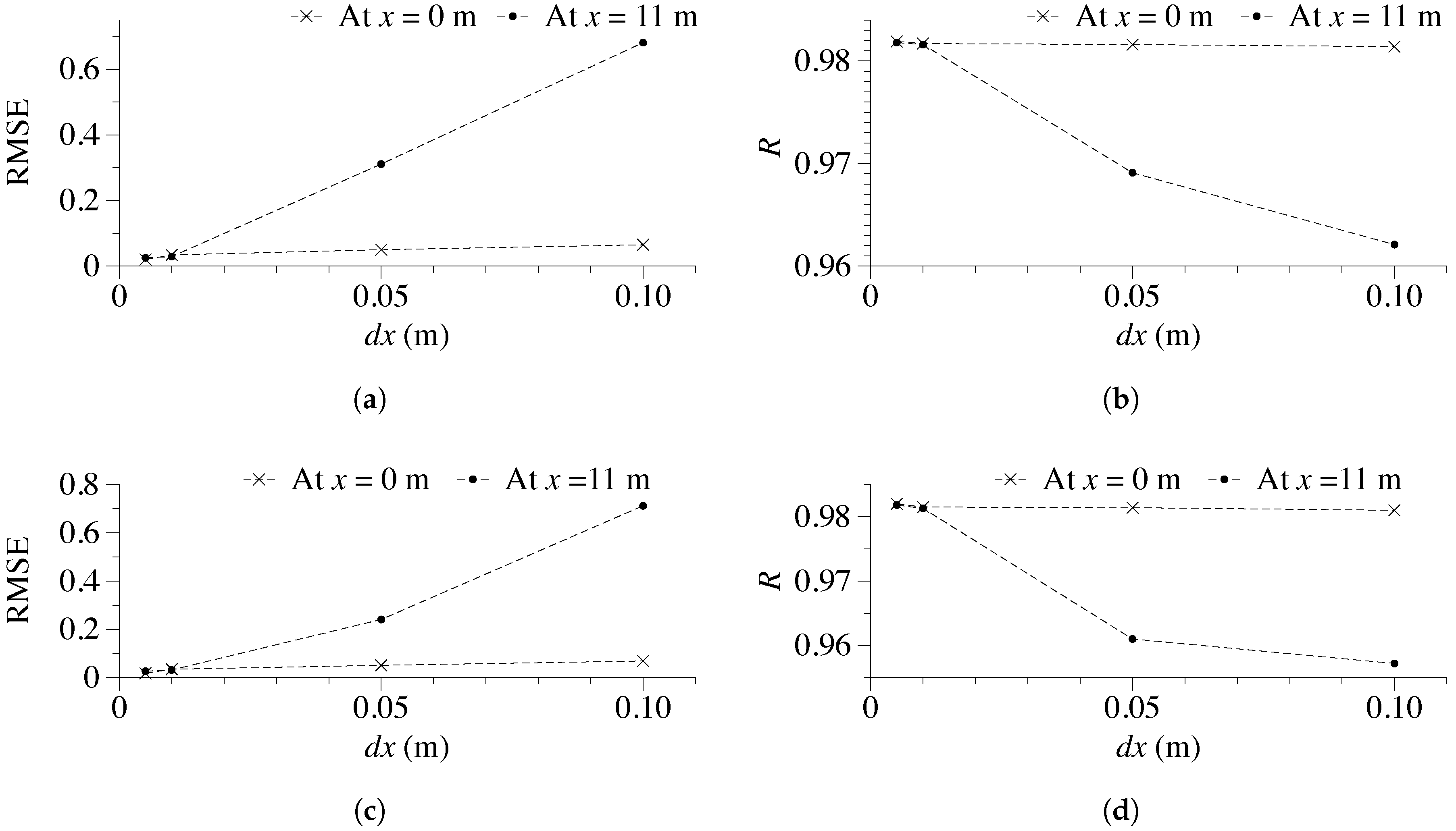
3.1. Grid Refinement Study with the Theoretical Input

In this section, the numerical simulations are performed for the verification of the free surface reconstruction method for irregular waves. The tests are conducted for two different wave steepness cases to verify the applicability of the reconstruction technique for four different grid sizes listed in

Table 1. List of simulation cases for theoretical inputs.

Case	Sim. No.	Significant Wave Height ${\mathit{H}}_{\mathit{s}}$ (m)	Peak Period ${\mathit{T}}_{\mathit{p}}$ (s)	Steepness s	Grid Size $\mathit{d}$ (m)
A	1	0.04	1.2	0.0178	0.10
	2				0.05
	3				0.01
	4				0.005
B	1	0.08	1.2	0.0356	0.10
	2				0.05
	3				0.01
	4				0.005

. The spectral wave steepness s for the irregular waves is defined as:

$$s=\frac{2\pi H_s}{g{T}_p^2},$$

(22)

where $H_s$ is the significant wave height and $T_p$ is the peak period.

A two-dimensional numerical wave tank (NWT) with a flat bed is employed for carrying out the simulations. The NWT is 15 m long and 1 m deep and the still water level is set to be d = 0.5 m. The setup of the NWT with the wave gauge locations is shown in Figure 1. The input theoretical irregular waves are generated using the JONSWAP spectrum with $H_s$ = 0.04 m and $T_p$ = 1.2 s (case A). All simulations are run for t = 200 s with the number of waves N = 499. The Courant—Friedrichs—Lewy (CFL) number is kept to be 0.1 for all the simulations, which has shown to give accurate results under all wave conditions [34].

The procedure to test the wave generation for the theoretical input with the free surface reconstruction method is summarised with the following steps:

• Simulation 1: Irregular waves are numerically simulated with a given significant wave height $H_s$ and peak period $T_p$ in the numerical model using the random wave phases with the JONSWAP spectrum. The numerical free surface elevation is measured at the different wave gauge locations along the NWT (x = 0 m and 11 m).
• Simulation 1: Free surface reconstruction algorithm is applied in this step to compute the wave amplitudes $A_i$, wave phases ${\varphi }_i$ and wave frequencies ${\omega }_i$ for the free surface elevation measured at x = 0 m using Equations (7)–(10).
• Simulation 2: The computed $A_i$, ${\varphi }_i$ and ${\omega }_i$ from simulation 1 are used as inputs to reproduce the waves in step 1 using Equations (14)–(17).
• Simulation 2: Finally, the waves generated using the free surface reconstruction method (simulation 2) are compared with the waves generated using the wave spectrum in the time-domain (simulation 1).

The numerical simulations are conducted for four different grid sizes $dx$ = 0.10 m (case A1), 0.05 m (case A2), 0.01 m (case A3) and 0.005 m (case A4) for the grid refinement study. Figure 2 presents the comparison of the numerically reconstructed and theoretical irregular wave free surface elevation versus time for the grid sizes $dx$ = 0.10 m, 0.05 m, 0.01 m and 0.005 m for case A. The results are shown for two wave gauges located at x = 0 m and x = 11 m to verify the wave generation and wave propagation along the NWT. For the wave gauge located at x = 0 m, the numerical model is able to reconstruct the input theoretical signal with a good accuracy at all grid sizes $dx$ (Figure 2a). When waves propagate along the NWT, the numerical results with coarser grids $dx$ = 0.10 m and 0.05 m are unable to represent the waves accurately at x = 11 m. The lack of a sufficient number of cells per wavelength lead to such numerical wave attenuation. The wave amplitude is damped out and the wave phases are not correctly captured with the coarser grid sizes. With finer grid sizes $dx$ = 0.01 m and 0.005 m, the numerical irregular wave surface elevation is described at x = 11 m with a good accuracy. The wave amplitudes, wave frequencies and wave phases are precisely reproduced and a good comparison with the theoretical wave signals is observed.

Furthermore, the capability of the wave reconstruction for case B with larger spectral steepness is investigated. The number of individual wave components in the irregular wave train with larger individual steepness increases indicating larger wave nonlinearity. In order to test this technique for steeper waves, the simulations are performed for case B. The numerical tests are performed for waves with $H_s$ = 0.08 m and $T_p$ = 1.2 s at three different grid sizes $dx$ = 0.10 m (case B1), 0.05 m (case B2), 0.01 m (case B3) and 0.005 m (case B4). Figure 3 presents the comparison of the numerically reconstructed and theoretical irregular wave free surface elevation versus time with grid sizes $dx$ = 0.10 m, 0.05 m, 0.01 m and 0.005 m for case B. The numerical results at x = 0 m indicate that the theoretical wave is reproduced with an acceptable accuracy, irrespective of the grid size ($dx$) (Figure 3a). However, at x = 11 m, the waves generated with the coarser grid sizes $dx$ = 0.10 m and 0.05 m do not show a good comparison with theory. The wave amplitudes and wave phases are not correctly computed in the numerical model at these grid sizes. For $dx$ = 0.10 m, significant differences are observed between the numerical results and theory, when wave propagates along the NWT. The numerical results with grid sizes $dx$ = 0.01 m and 0.005 m are in a good agreement with theory; the numerical model is able to reproduce the irregular wave train with steep wave components at x = 11 m. The results do not significantly change between $dx$ = 0.01 m and $dx$ = 0.005 m. This demonstrates that the numerical solution is converged at $dx$ = 0.01 m. Therefore, the grid size $dx$ = 0.01 m is used for the further simulations in the present study.

Furthermore, an error analysis is performed in order to quantify the differences between the reconstructed and the target free surface elevation. The root-mean-square error (RMSE) for the wave phases is computed and a correlation coefficient (R) is also determined to estimate the accuracy of the numerical free surface elevation. The value of $R=1$ means exact match between two wave signals. It can be defined as:

$$\rho ({\eta }_i^{re},{\eta }_i^{ta})=\frac{({\eta }_i^{re},{\eta }_i^{ta})}{{\sigma }_{{\eta }_i^{re}}{\sigma }_{{\eta }_i^{ta}}},$$

(23)

where ${\eta }_i^{ta}$ is the target (theoretical or experimental) irregular free surface elevation and ${\eta }_i^{re}$ is the numerically reconstructed free surface elevation, ${\sigma }_{{\eta }_i^{re}}$ and ${\sigma }_{{\eta }_i^{re}}$ are the standard deviations for ${\eta }_i^{ta}$ and ${\eta }_i^{ta}$, respectively. The correlation coefficient matrix of two random variables is the matrix of correlation coefficients for each pairwise variable combination:

$$R=\left[\begin{array}{cc}\rho ({\eta }_i^{re},{\eta }_i^{re})& \rho ({\eta }_i^{re},{\eta }_i^{ta})\\ \rho ({\eta }_i^{ta},{\eta }_i^{re})& \rho ({\eta }_i^{ta},{\eta }_i^{ta})\end{array}\right].$$

${\eta }_i^{re}$ and ${\eta }_i^{ta}$ are always directly correlated to themselves, that is:

$$R=\left[\begin{array}{cc}1& \rho ({\eta }_i^{re},{\eta }_i^{ta})\\ \rho ({\eta }_i^{ta},{\eta }_i^{re})& 1\end{array}\right].$$

Figure 4 presents the RMSE (computed for wave phases) and correlation coefficient (R) between the numerical reconstructed and theoretical wave free surface elevation versus grid size for cases A and B. The differences between the errors for different $dx$ are very small for the wave measured at x = 0 m. The numerical model is able to generate reasonably accurate waves at all grid sizes $dx$. The errors observed are almost negligible for both cases. At x = 11 m, the numerical error is significantly reduced and the correlation coefficient R also becomes closer to 1 by refining the mesh from $dx$ = 0.10 m to $dx$ = 0.01 m (Figure 4a,b). For case B with larger spectral steepness, the observed error is larger than for waves with lower spectral steepness (case A) at $dx$ = 0.10 m (Figure 4c). This is due to the insufficient cells per wave component to account for the wave nonlinearity. The numerical results at coarser grid sizes are unable to model these wave components, which lead to higher errors in the free surface elevation. The numerical error is reduced by 140 times and the value of R becomes very close to 1 on reducing $dx$ to 0.01 m from $dx$ = 0.10 m (Figure 4d). However, further improvement in the numerical results on refining the grid size $dx$ to 0.005 m is almost negligible because the numerical solution converges at $dx$ = 0.01 m. The highly nonlinear wave components evolve during the propagation of the irregular wave group with the large spectral steepness. For further larger wave steepness cases, the increase in the accuracy of the results on refining $dx$ could be relatively more due to the presence of wave components with further larger individual wave height and wavelength in the irregular wave train.

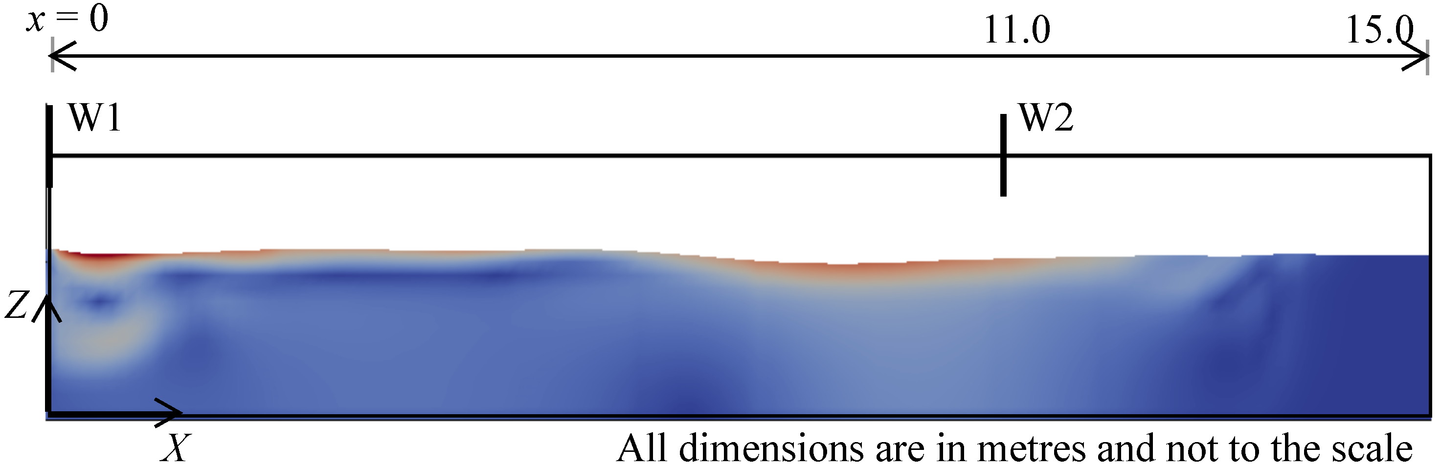
3.2. Breaking Irregular Waves over a Submerged Bar

Wave transformation takes place when waves propagate from deep to shallow water due to the change in water depth. In case of irregular waves, the higher harmonics emerged during nonlinear wave–wave interaction throughout the shoaling and breaking processes interact with the incident individual wave components. Therefore, the capability of the proposed free surface reconstruction method to model the wave transformation process and resulting wave amplitudes and wave phases in the time-domain without a prior information of wavemaker kinematics is tested. In order to validate the present approach, the numerically reconstructed irregular wave signal at different wave gauge locations is compared with the experiments performed by Beji and Battjes [38] in the time-domain for breaking irregular waves in shallow water. The data for breaking regular waves and non-breaking irregular waves from the same experiment has also been used in previous studies [3,5,58,59]. The numerical simulations are performed in a two-dimensional NWT that is 27 m long and 0.8 m high. The water depth (d) is 0.4 m. The numerical setup is similar to the experimental setup. Six wave gauges are positioned to measure the free surface elevation at different wave gauge locations along the length of the wave flume. The numerical setup is demonstrated in Figure 5.

The experiments were performed for irregular waves with $H_s$ = 0.054 m and $T_p$ = 2.5 s using the JONSWAP spectrum. The wave gauge at x = 6 m measures the free surface elevation before the submerged bar. In order to compute the experimental wave phases, wave amplitudes and frequencies at x = 0 m, the linear dispersion relationship is assumed (${\omega }_i=\sqrt{g{k}_i\tanh k_{i}d}$) for the wave propagation as follows:

• The wave amplitudes ($A_i$), wave phases (${\varphi }_i^{6m}$) and wave frequencies (${\omega }_i$) are computed from the experimental free surface elevation at x = 6 m.
• With an assumption of linear dispersion between x = 0 m and 6 m (from the wave generation until the waves interact with the bar), the wave phases at x = 0 m (${\varphi }_i^{0m}$) are computed by using the equation: ${\varphi }_i^{0m}={\varphi }_i^{6m}-k_{i}x$, where x = −6 m.
• The computed wave phases ${\varphi }_i^{0m}$, wave amplitudes ($A_i$) and wave frequencies (${\omega }_i$) are used as inputs to the numerical model for the wave generation.
• The numerical free surface elevation is compared with the experimental free surface elevation at different wave gauge locations along the wave tank.

Figure 6 presents the comparison of the numerically reconstructed and the experimental free surface elevation versus time at six different wave gauge locations. The numerical tests are conducted for the grid size $dx$ = 0.01 m. The wave gauge at x = 6 m (W1) measures the free surface elevation before the depth induced wave transformation (before the bar) (Figure 6a). The wave amplitudes, frequencies and wave phases are reproduced reasonably well in the numerical model. When the waves propagate over the bar, the water depth reduces which leads to wave shoaling. The shoaling process leads to an increase in the wave heights. Due to this, the wave profile becomes nonlinear and the wave crests become sharp, indicating the presence of higher-order components in the irregular wave train (Figure 6b). The water depth reduces further and the irregular wave train experiences more shoaling until they reach the flat part of the bar. The contribution of the higher-harmonics becomes pronounced as illustrated by the nonlinear and sharper wave crests (Figure 6c). The water depth is reduced by 75% at the flat part of the bar, the wave crests of few waves in the wave train become steep and the front faces become nearly vertical as noticed in Figure 7b and collapses forward due to the instability induced in the wave crest leading to wave breaking (Figure 7c). The wave breaking process tends to dissipate the wave energy. In addition, many short wave components are generated during this process (Figure 7d). This is seen from the wave signals at x = 12 m and 13 m, that the steep wave components break resulting in the dissipation of wave energy (Figure 6d,e). The present numerical technique models the breaking process in the time-domain with reasonably accurate phases, frequencies and amplitudes. After the waves propagate over the flat bed of the bar, the water depth increases and wave deshoaling occurs. The waves are further decomposed into multiple frequencies (secondary and tertiary components) and a significant amount of wave energy is transferred towards higher-harmonics. Some small phase differences are observed between the numerical and experimental irregular wave signal at x = 16 m, but are well within the range of reasonable accuracy. It can be inferred that the present wave reconstruction approach employed in the numerical model is able to represent the complex wave transformation processes including wave shoaling, wave breaking, wave deshoaling and wave decomposition for breaking irregular waves propagating over a submerged bar.

In order to further investigate the errors between the numerically reconstructed and the experimental wave signal, the RMSE and the correlation coefficient R for the free surface elevation at each wave gauge location is estimated. Figure 8 presents the RMSE and the correlation coefficient R between the numerically reconstructed and experimental wave free surface elevation for the submerged bar case. It is clearly noticed that the computed errors at all wave gauge locations are quite small and the value of R is close to 1. However, the relative magnitude of errors grows gradually which is also noticed by a decrease in the value of R. The errors computed until the wave gauge located at x = 13 m (W4) are negligible, and the increase of error compared to the preceding wave gauge is low. This highlights the fact that the wave components generated using the present wave reconstruction approach are able to represent wave shoaling with a very good accuracy. Most of the waves in the irregular wave train break at the wave gauge located at x = 14 m indicating increased nonlinear components and multiple frequencies in the post-breaking region. The increase in the computed error and the reduction in R value at this wave gauge is relatively higher than the preceding wave gauges owing to the complex wave breaking process. In addition to that, the main wave components undergo a wave decomposition process during the propagation over the lee side of the bar due to increased water depth and wave deshoaling process.

3.3. Irregular Waves with Large Spectral Steepness in Deep Water

The higher-order nonlinear interactions play important roles in the evolutions of gravity waves in deep water. They can transfer energy among the Fourier modes and excite chaotic mode evolutions. Their role in influencing the maximum wave height $H_{max}$ and kurtosis is also significant. They can lead to a larger wave height in deep water compared to the Rayleigh theory predictions [60]. This makes the study of irregular waves with large spectral steepness in deep water highly relevant. In this part, the applicability of the present free surface reconstruction approach to reproduce the irregular waves with large spectral steepness in deep water is demonstrated. The numerical results are compared with the experiments by Pákozdi et al. [39]. In the experiments, the steep irregular waves with $H_s$ = 0.345 m and $T_p$ = 2.6 s were generated using the Torsethaugen spectrum [61]. The numerical investigation is performed in a two-dimensional NWT, which is 40 m long and 15 m deep with a flat bed. The still water level is taken at d = 10 m (Figure 9). The wave propagation of irregular waves with large spectral steepness in deep water can be seen in Figure 10. The wave gauges are positioned at x = 1.4 m (W1), 15.0 m (W2) and 34.74 m (W3) to measure the free surface elevation at different wave gauge locations along the NWT. The wave phases and amplitudes at x = 0 m, which are used as inputs to the numerical model, are computed following the same steps as explained in Section 3.2 from the experimental free surface elevation at x = 1.4 m.

Figure 11 presents the comparison between the numerically reconstructed and experimental wave free surface elevation versus time at different wave gauge locations. The numerical model is able to generate the time-history of the irregular wave train with highly nonlinear wave components in deep water using the wave reconstruction technique. This is noticed by a reasonable comparison of the free surface at the wave gauge located next to the wavemaker (W1) (Figure 11a). This is also highlighted by the low RMSE and high R (close to 1) values at this wave gauge location as shown in Figure 12. When the waves propagate further along the NWT, they experience higher-order wave–wave interactions leading to a highly nonlinear irregular wave train. The Torsethaugen spectrum also contains swell waves indicating the role of longer waves influencing sea waves. The swell-sea wave interaction leads to the generation of several wave components with steeper wave crests during the wave propagation (Figure 11b). The present numerical approach simulates the whole process of higher-order wave–wave interaction with a good accuracy (Figure 11c). The RMSE computed at the wave gauge locations farther from the wave generation are very low (Figure 12a) and the value of R is quite close to 1. However, a small increment in the errors is observed. This is due to the nonlinear interaction of swell with sea waves. Overall, the numerical results illustrate a good comparison with the experimental results for all wave gauge locations with low errors.

3.4. Irregular Wave Forces on a Monopile

The present approach to reconstruct the free surface elevation can also be applied for numerically simulating experimental irregular wave forces in the time-domain. In order to exactly model the experimental irregular wave force signal in the time-domain with the correct phases, the numerically reconstructed irregular free surface elevation before interacting with a structure should be consistent with its experimental counterpart. The numerical results are compared with the experiments performed on a model scale of 1:40 at SINTEF Ocean [40]. A monopile with a diameter of D = 0.175 m was used in the experimental setup. The numerical tests are performed in a three-dimensional NWT with a modified fluid domain in order to reduce the computational costs. The NWT of 13 m length, 1 m width and 2 m height with the still water level at d = 0.75 m is utilized in this study. Three wave gauges are installed at x = 0 m (W1), 2.5 m (W2) and 5.0 m (W3) along the NWT to study the changes in the free surface elevation during the wave-cylinder interaction process (Figure 13). Figure 14 presents snapshots of the numerically reconstructed free surface during the interaction of the irregular wave crest with the cylinder. The waves experience reflections from the cylinder, which is noticed by a narrow water jet towards the incident wave direction, when the wave crest is besides the cylinder (Figure 14d).

Figure 15 presents the numerically reconstructed and experimental wave free surface elevation at different wave gauge locations along the NWT in both the time and frequency domains. The wave gauge at x = 0 m (W1) measures the free surface elevation at the wave generation (located far from the cylinder) (Figure 15a). The numerical waves are in good agreement with the experimental waves at W1. The spectral peaks and the wave energy distribution at all frequencies are well reproduced (Figure 15b). The primary peak in the wave spectral density corresponds to the peak frequency of the irregular wave train. There are some irregularities in the wave spectra which are most likely due to the size of the sampling interval used for smoothening of the wave spectra. The observed RMSE for wave phases computed at W1 is almost negligible and value of R is almost 1 illustrating the reasonable accuracy of the phases, amplitudes and frequencies of numerically generated irregular waves (Figure 16). When waves propagate further towards the cylinder, they experience reflections from the cylinder. These reflected waves interact with the incident waves and further influence their phases, amplitudes and frequencies. Some small differences in wave phases are observed in the numerical free surface elevation computed for the wave gauge located at W2 (Figure 15c), but, overall, the present free surface reconstruction method is able to model the irregular wave train at W2 with reasonable accuracy in both the time and frequency domains. The computed RMSE computed at x = 2.5 m (W2) is relatively higher compared to the one at W1. The increase in the error is due to the nonlinear interaction of reflected waves with the incident waves. A primary peak in the wave spectrum at peak frequency f = 1.08 Hz is observed for both experimental and numerical wave spectra (Figure 15d). The contribution of the longer waves in the wave spectral density increases at this wave gauge location as observed by the highlighted secondary peak at f = 0.95 Hz. The wave gauge located at x = 5 m (W3, Figure 15e) computes the free surface elevation during the interaction of irregular waves with the cylinder. The numerically reconstructed waves also reproduce the modified irregular wave surface elevation in the vicinity of the cylinder (during the wave–cylinder interaction) correctly. The computed RMSE at this wave gauge location is low and the value of R is satisfactory. It is noticed from the experimental and numerical wave spectra that the spectral peaks are shifted towards lower frequencies and the secondary peaks become more evident due to the nonlinear wave-structure interaction (Figure 15f). In addition, the value of the peak spectral density is reduced compared to the peak spectral density at W1 due to the wave energy dissipation in the form of turbulence and heat.

Figure 17 presents the numerically reconstructed and experimental irregular wave force on the cylinder versus time. The structural response was also measured in the experiments due to the observed ringing phenomenon. The structural response values are taken out from the experimental force data in the frequency-domain by removing the force values at the ringing frequency in order to compare the wave forces. The force peaks and the phases in the experimental force signal are simulated reasonably with the present approach (Figure 17a). The computed free surface elevation at W3 (located besides the cylinder) is composed of the incident and reflected waves. These phenomena in the free surface elevation induce nonlinearities in the force signal. It is evident in Figure 17b that the higher-harmonics in the free surface elevation induce multiple peaks in the force spectrum. The primary peak at f = 1.08 Hz corresponds to the dominant frequency in the irregular wave train. The secondary and tertiary peaks in the lower and higher frequencies are generated due to the nonlinear wave-structure interaction. The secondary and tertiary peaks in the force spectra are relatively low in magnitude but can play a very important role in influencing the structural response. The present numerical approach computes the nonlinear irregular wave forces with accurate force peaks, frequencies and phases. Overall, the current approach to reconstruct the phase accurate irregular free surface elevation in the time-domain without the information of experimental wavemaker kinematics can be applied to three-dimensional problems. However, despite of good numerical results, it should be kept in mind that the classical eddy-viscosity based models developed for wall-bounded high-Reynolds number turbulence have limitations in accurately modeling the complex physics involved in the vortex interactions and the effects of pressure fluctuations on the interface [62,63]. The use of eddy-viscosity based two-equation models introduces a level of discrepancy due to the inability of such models to capture complex interactions arising due to turbulence anisotropy and eigenvector misalignment [64,65]. However, most CFD investigations for the free-surface simulations still rely on such models by precedent [66]. The present study is conducted with this precedent and rely on two-equation eddy-viscosity turbulence models to replicate the results that would be observed in an industrial application.

4. Conclusions

An approach to reconstruct the phase accurate irregular free surface elevation coupled with Dirichlet inlet boundary condition is presented. A two-phase CFD model is used to generate irregular waves with the proposed method. First, a grid refinement study is performed to verify the present approach to generate phase accurate irregular waves with different grid sizes in order to choose the optimal grid size. This is achieved by comparing the numerically reconstructed free surface elevation with the theory at different wave gauge locations. The simulations with multiple grid sizes are conducted for two different wave steepnesses. The RMSE and R values are computed at different grid sizes to further quantify the differences between the numerical and experimental results. Next, the current technique is utilized to model breaking irregular waves over a submerged bar. The numerical irregular free surface elevations during the wave transformation process are in good agreement with the experimental data with low RMSE and high R. The phases of higher-order harmonics evolved during wave shoaling, wave breaking and wave deshoaling processes are captured with reasonable accuracy. The nonlinear energy transfers to the Fourier nodes and higher-order wave–wave interaction become quite important for the investigation of deep water waves. The performance of the numerical free surface reconstruction for the deep water benchmark case appears to be quite satisfactory; this is demonstrated by the accurate wave phases (low RMSE) and high R in the numerically reconstructed free surface elevation.

Furthermore, this approach is applied for the modelling of a three-dimensional wave tank problem to estimate the irregular wave forces on a cylinder. The irregular wave train at the locations away from the cylinder and in the proximity of the cylinder is correctly represented by the numerical model in the time-domain. The interaction of the reflected waves from the cylinder with the incident waves is well simulated indicated by a good agreement of the experimental and numerical wave spectral densities. The secondary peak in the wave spectral density is pronounced at the cylinder due to the nonlinear wave–cylinder interaction in the irregular wave train. The numerical and experimental force signals are further compared in the frequency domain to investigate the capability of this approach to simulate the wave forces at all frequencies and a good agreement with the experiments is observed. The pronounced secondary peaks in the wave spectral density at the cylinder contribute to the higher-order force harmonics. Overall, all the benchmark cases demonstrate the capability of the proposed approach to generate phase accurate irregular waves for different applications: breaking irregular waves, deep water irregular waves with larger spectral steepness and irregular wave forces.

References

1. Massel, R. Ocean Surface Waves: Their Physics and Prediction; World Scientific: Singapore, 1996. [Google Scholar]
2. Thomas, J.; Dwarakish, S. Numerical wave modelling: A review. Aquat. Procedia 2015, 4, 443–448. [Google Scholar] [CrossRef]
3. Eldeberky, Y.; Battjes, A.J. Nonlinear coupling in waves propagating over a bar. Coast. Eng. 1994. [Google Scholar] [CrossRef]
4. Hu, Z.Z.; Causon, D.M.; Mingham, C.G.; Qian, L. Numerical simulation of floating bodies in extreme free surface waves. Nat. Hazards Earth Syst. Sci. 1985, 11, 519–527. [Google Scholar] [CrossRef] [Green Version]
5. Beji, S.; Battjes, J. Numerical simulation of nonlinear wave propagation over a bar. Coast. Eng. 1994, 23, 1–16. [Google Scholar] [CrossRef]
6. Harlow, H.F.; Welch, E.J. Numerical calculation of time dependent viscous incompressible flow of fluid with free surface. Phys. Fluids 1965, 8, 2182–2165. [Google Scholar] [CrossRef]
7. Lee, H.S.; Kwon, H.S. Wave profile measurement by wavelet transform. Ocean Eng. 2003, 30, 2313–2328. [Google Scholar] [CrossRef]
8. West, B.J.; Brueckner, K.A.; Janda, R.S. A numerical method for surface hydrodynamics. J. Geophys. Res. 1987, 92, 11803–11824. [Google Scholar] [CrossRef]
9. Dean, R.G. Stream function representation of nonlinear ocean waves. J. Geophys. Res. 1965, 70, 4561–4572. [Google Scholar] [CrossRef]
10. Tromans, S.; Anaturk, R.A.; Hagemeijer, P. A new model for the kinematics of large ocean waves—Application as a design wave. In Proceedings of the First International Offshore and Polar Engineering Conference. International Society of Offshore and Polar Engineers, Edinburgh, UK, 11–16 August 1991. [Google Scholar]
11. Massel, R. Wavelet analysis for processing of ocean surface wave records. Ocean Eng. 2001, 28, 957–987. [Google Scholar] [CrossRef]
12. Kao, S. Governing equations and spectra for atmospheric motion and transports in frequency-wavenumber space. J. Atmos. Sci. 1968, 25, 32–38. [Google Scholar] [CrossRef]
13. Kao, S.; Wendell, L. The kinetic energy of the large-scale atmospheric motion in wavenumber-frequency space: I. Northern hemisphere. J. Atmos. Sci. 1970, 27, 359–375. [Google Scholar] [CrossRef]
14. Brandt, A.; Ramberg, S.E.; Shlesinger, F.M. Nonlinear Dynamics of Ocean Waves; World Scientific: Singapore, 1992. [Google Scholar]
15. Kinsman, B. Wind Waves; Prentice-Hall: Eaglewood Cliffs, NJ, USA, 1965. [Google Scholar]
16. Bendat, S.; Piersol, G. Random Data: Analysis and Measurement Procedures; Wiley-Interscience: New York, NY, USA, 1971. [Google Scholar]
17. Svendsen, I. Physical modelling of water waves. In Physical Modelling in Coastal Engineering; AA Balkema: Rotterdam, The Netherlands, 1985; pp. 13–48. [Google Scholar]
18. Lubin, P.; Vincent, S.; Abadie, S.; Caltagrione, J. Three-dimensional LES simulation of air entrainment under plunging breaking waves. Coast. Eng. 2006, 53, 631–655. [Google Scholar] [CrossRef]
19. Christensen, E.D. LES simulation of spilling and plunging breakers. Coast. Eng. 2006, 53, 463–485. [Google Scholar] [CrossRef]
20. Jacobsen, N.G.; Fuhrman, D.; Fredsøe, J. A wave generation toolbox for the open-source CFD library: OpenFoam®. Int. J. Numer. Methods Fluids 2012, 70, 1073–1088. [Google Scholar] [CrossRef]
21. Alagan Chella, M.; Bihs, H.; Myrhaug, D. Characteristics and profile asymmetry properties of waves breaking over an impermeable submerged reef. Coast. Eng. 2015, 100, 26–36. [Google Scholar] [CrossRef]
22. Alagan Chella, M.; Bihs, H.; Myrhaug, D.; Michael, M. Hydrodynamic characteristics and geometric properties of plunging and spilling breakers over impermeable slopes. Ocean Model. 2016, 103, 53–72. [Google Scholar] [CrossRef]
23. Li, S.; Liu, X.; Yu, X.; Lai, Z. Numerical modelling of multi-directional irregular waves through breakwaters. Appl. Math. Model. 2000, 24, 551–574. [Google Scholar] [CrossRef]
24. Aggarwal, A.; Alagan Chella, M.; Kamath, A.; Bihs, H.; Arntsen, Ø.A. Irregular Wave Forces on a Large Vertical Circular Cylinder. Energy Procedia 2016, 94, 504–516. [Google Scholar] [CrossRef]
25. Lara, L.; Garcia, N.; Losada, J. RANS modelling applied to random wave interaction with submerged permeable structures. Coast. Eng. 2006, 53, 395–417. [Google Scholar] [CrossRef]
26. Panchang, G.; Wei, G.; Pearce, R.; Briggs, J. Numerical simulation of irregular wave propagation over shoal. J. Waterw. Port Coast. Ocean Eng. 1990, 116, 324–340. [Google Scholar] [CrossRef]
27. Paulsen, T.B.; Bredmose, H.; Bingham, B.H.; Schløer, S. Steep wave loads from irregular waves on an offshore wind turbine foundation: Computation and experiment. In Proceedings of the 32nd International Conference on Ocean, Offshore and Arctic Engineering, American Society of Mechanical Engineers, Nantes, France, 9–14 June 2013. [Google Scholar]
28. Paulsen, T.B.; Bredmose, H.; Bingham, B.H. An efficient domain decomposition strategy for wave loads on surface piercing circular cylinders. Coast. Eng. 2014, 86, 57–76. [Google Scholar] [CrossRef]
29. Bredmose, H.; Jacobsen, G.N. Breaking wave impacts on offshore wind turbine foundations: focused wave groups using CFD. In Proceedings of the 29th International Conference on Ocean, Offshore and Arctic Engineering, American Society of Mechanical Engineers, Shanghai, China, 6–11 June 2010. [Google Scholar]
30. Bredmose, H.; Hunt-Ruby, A.; Jayaratne, R. The ideal flip-through impact: Experimental and numerical investigation. J. Eng. Math. 2010, 67, 115–136. [Google Scholar] [CrossRef]
31. Goda, Y.; Suzuki, Y. Estimation of incident and reflected wave in random wave experiment. In Proceedings of the 15th International Conference on Coastal Engineering, Honolulu, HI, USA, 11–17 July 1976. [Google Scholar]
32. Mansard, E.; Funke, E. The measurement of incident and reflected spectra using a least squares method. In Proceedings of the 17th International Conference on Coastal Engineering, Sydney, Australia, 23–28 March 1980. [Google Scholar]
33. Buldakov, E.; Stagonas, D.; Simons, R. Extreme wave groups in a wave flume: controlled generation and breaking onset. Coast. Eng. 2017, 128, 75–83. [Google Scholar] [CrossRef]
34. Bihs, H.; Kamath, A.; Alagan Chella, M.; Aggarwal, A.; Arntsen, Ø.A. A new level set numerical wave tank with improved density interpolation for complex wave hydrodynamics. Comput. Fluids 2016, 140, 191–208. [Google Scholar] [CrossRef]
35. Bihs, H.; Kamath, A.; Alagan Chella, M.; Arntsen, Ø.A. Breaking-wave interaction with tandem cylinders under different impact scenarios. J. Waterw. Port Coast. Ocean Eng. 2016, 142, 04016005. [Google Scholar] [CrossRef]
36. Alagan Chella, M.; Bihs, H.; Myrhaug, D.; Muskulus, M. Breaking solitary waves and breaking wave forces on a vertically mounted slender cylinder over an impermeable sloping seabed. J. Ocean Eng. Mar. Energy 2017, 3, 1–19. [Google Scholar] [CrossRef]
37. Aggarwal, A.; Alagan Chella, M.; Kamath, A.; Bihs, H.; Arntsen, Ø.A. Numerical simulation of irregular wave forces on a horizontal cylinder. In Proceedings of the ASME 35th International Conference on Ocean, Offshore and Arctic Engineering, Busan, Korea, 19–24 June 2016. [Google Scholar]
38. Beji, S.; Battjes, J. Experimental investigation of wave propagation over a bar. Coast. Eng. 1993, 19, 151–162. [Google Scholar] [CrossRef]
39. Pákozdi, C.; Visscher, J.H.; Stansberg, C.; Fagertun, J. Experimental investigation of global wave impact loads in steep random seas. In Proceedings of the 25th International Ocean and Polar Engineering Conference, International Society of Offshore and Polar Engineers, Kona, HI, USA, 21–26 June 2015. [Google Scholar]
40. Pákozdi, C.; Spence, S.; Fouques, S.; Thys, M.; Alsos, S.H.; Bachynski, E.E.; Bihs, H.; Kamath, A. Nonlinear wave load models for extra large monopiles. In Proceedings of the 1st International Offshore Wind Technical Conference, San Francisco, CA, USA, 4–7 November 2018. [Google Scholar]
41. Jiang, G.S.; Peng, D. Weighted ENO schemes for Hamilton Jacobi equations. SIAM J. Sci. Comput. 2000, 21, 2126–2143. [Google Scholar] [CrossRef]
42. Shu, C.; Gottlieb, S. Total variation diminishing Range Kutta schemes. Math. Comput. 1998, 67, 73–85. [Google Scholar]
43. Griebel, M.; Dornseifer, T.; Neunhoeffer, T. Numerical Simulations in Fluid Dynamics; SIAM: Philadelphia, PA, USA, 1998. [Google Scholar]
44. Wilcox, D. Turbulence Modeling for CFD; DCW Industries Inc.: La Canada, CA, USA, 1994. [Google Scholar]
45. Durbin, P. Limiters and wall treatments in applied turbulence modeling. Fluid Dyn. Res. 2009, 41, 012203. [Google Scholar] [CrossRef]
46. Osher, S.; Sethian, J.A. Fronts propagating with curvature- dependent speed: Algorithms based on hamilton-jacobi formulations. J. Comput. Phys. 1988, 79, 12–49. [Google Scholar] [CrossRef]
47. Berthelsen, P.A.; Faltinsen, O.M. A local directional ghost cell approach for incompressible viscous flow problems with irregular boundaries. J. Comput. Phys. 2008, 227, 4354–4397. [Google Scholar] [CrossRef]
48. Bihs, H.; Kamath, A. A combined level set/ghost cell immersed boundary representation for simulations of floating bodies. Int. J. Numer. Methods Fluids 2017, 83, 905–916. [Google Scholar] [CrossRef]
49. Schaffer, A.H.; Klopman, G. Review of multidirectional active wave absorption methods. J. Waterw. Port Coast. Ocean Eng. 2000, 126, 88–97. [Google Scholar] [CrossRef]
50. Kamath, A.; Alagan Chella, M.; Bihs, H.; Muskulus, M. CFD investigations of wave interaction with a pair of large tandem cylinders. Ocean Eng. 2015, 108, 734–748. [Google Scholar] [CrossRef]
51. Ong, M.C.; Kamath, A.; Bihs, H.; Afzal, M.S. Numerical simulation of free-surface waves past two semi-submerged horizontal circular cylinders in tandem. Mar. Struct. 2017, 52, 1–14. [Google Scholar] [CrossRef]
52. Grotle, E.L.; Bihs, H.; Æsøy, V. Experimental and numerical investigation of sloshing under roll excitation at shallow liquid depths. Ocean Eng. 2017, 138, 73–85. [Google Scholar] [CrossRef]
53. Aggarwal, A.; Alagan Chella, M.; Bihs, H.; Pákozdi, C.; Petter, A.; Arntsen, O. CFD-based study of steep irregular waves for extreme wave spectra. Int. J. Offshore Polar Eng. 2017, 28, 164–170. [Google Scholar] [CrossRef]
54. Ahmad, N.; Bihs, H.; Myrhaug, D.; Kamath, A.; Arntsen, Ø.A. Three-dimensional numerical modelling of wave-induced scour around piles in a side-by-side arrangement. Coast. Eng. 2018, 138, 132–151. [Google Scholar] [CrossRef]
55. Hoffmann, J. MATLAB und Simulink; Addison Wesley Longman: Boston, MA, USA, 2009. [Google Scholar]
56. Newland, D.E. Random Vibrations, Spectral and Wavelet Analysis; Longman Scientific & Technical: Harlow, UK, 1993. [Google Scholar]
57. Dean, R.G.; Dalrymple, R.A. Water Wave Mechanics for Engineers and Scientists; World Scientific Publishing Co. Pte. Ltd.: Singapore, 2000. [Google Scholar]
58. Ohyama, T.; Beji, S.; Nadaoka, K.; Battjes, A.J. Experimental verification of numerical model for nonlinear wave evolutions. J. Port Waterw. Coast. Ocean Eng. 1994, 120, 637–644. [Google Scholar] [CrossRef]
59. Kamath, A.; Alagan Chella, M.; Bihs, H.; Arntsen, Ø.A. Energy transfer due to shoaling and decomposition of breaking and non-breaking waves over a submerged bar. Eng. Appl. Comput. Fluid Mech. 2017, 11, 450–466. [Google Scholar] [CrossRef]
60. Mori, N.; Yasuda, T. Effects of high-order nonlinear wave–wave interactions on gravity waves. In Proceedings of the Rogue Waves 2000: Proceedings of a Workshop, Brest, France, 29–30 November 2000; pp. 229–244. [Google Scholar]
61. Torsethaugen, K. Model for Double Peaked Wave Spectrum; SINTEF Report STF22 A96204; SINTEF: Trondheim, Norway, 1996. [Google Scholar]
62. Shirani, E.; Jafari, A.; Ashgriz, N. Turbulence models for flows with free surfaces and interfaces. AIAA J. 2006, 44, 1454–1462. [Google Scholar] [CrossRef]
63. Mishra, A.A.; Girimaji, S.S. Toward approximating non-local dynamics in single-point pressure–strain correlation closures. J. Fluid Mech. 2017, 811, 168–188. [Google Scholar] [CrossRef]
64. Oliver, T.A.; Moser, R.D. Bayesian uncertainty quantification applied to RANS turbulence models. J. Phys. Conf. Ser. 2011, 318, 042032. [Google Scholar] [CrossRef] [Green Version]
65. Iaccarino, G.; Mishra, A.A.; Ghili, S. Eigenspace perturbations for uncertainty estimation of single-point turbulence closures. Phys. Rev. Fluids 2017, 2, 024605. [Google Scholar] [CrossRef]
66. Ferreira, V.; Mangiavacchi, N.; Tomé, M.; Castelo, A.; Cuminato, J.; McKee, S. Numerical simulation of turbulent free surface flow with two-equation k–ε eddy-viscosity models. Int. J. Numer. Methods Fluids 2004, 44, 347–375. [Google Scholar] [CrossRef]
Figure 1. Numerical wave tank setup for the grid refinement study (coloured with the velocity contours).
Jmse 06 00105 g001
Figure 2. Comparison of the theoretical input and reconstructed irregular wave signal for case A (a) W1 (x = 0 m); (b) W2 (x = 11 m).
Jmse 06 00105 g002
Figure 3. Comparison of the theoretical input and reconstructed irregular wave signal for case B (a) W1 (x = 0 m); (b) W2 (x = 11 m).
Jmse 06 00105 g003
Figure 4. Comparison of accuracy between the numerical and experimental wave signal with different grid sizes d x for (a) case A (RMSE for wave phases); (b) case A (R); (c) case B (RMSE for wave phases); (d) case B (R).
Jmse 06 00105 g004
Figure 5. Numerical wave tank setup for simulating the experiments performed by Beji and Battjes [38].
Jmse 06 00105 g005
Figure 6. Comparison of the experimental and reconstructed irregular wave signal for breaking irregular waves (a) W1 (x = 6 m); (b) W2 (x = 11 m); (c) W3 (x = 12 m); (d) W4 (x = 13 m); (e) W5 (x = 14 m); (f) W6 (x = 16 m).
Jmse 06 00105 g006
Figure 7. Numerically reconstructed irregular wave free surface over a submerged bar (zoomed around the free surface) at t / T p = (a) 19.14 s; (b) 19.32; (c) 19.58; (d) 19.85.
Jmse 06 00105 g007
Figure 8. Comparison of accuracy between the numerical and experimental wave signal at different wave gauge positions by (a) RMSE for wave phases; (b) R.
Jmse 06 00105 g008
Figure 9. Numerical wave tank setup for simulating the experiments performed by Pákozdi et al. [39] (side-view).
Jmse 06 00105 g009
Figure 10. Snapshots of numerically reconstructed steep irregular wave propagating in deep water in side view at (a) t = 38.37 s; (b) t = 38.37 s (zoomed around the free surface); (c) t = 38.69 s (zoomed around the free surface).
Jmse 06 00105 g010
Figure 11. Comparison of the numerically reconstructed and experimental irregular wave signal for steep irregular waves in deep water at (a) W1 (x = 1.4 m); (b) W2 (x = 15 m); (c) W3 (x = 34.74 m).
Jmse 06 00105 g011
Figure 12. Comparison of accuracy between the numerical and experimental wave signal at different wave gauge positions by (a) RMSE for wave phases; (b) R.
Jmse 06 00105 g012
Figure 13. Numerical wave tank setup for simulating the experiments performed at SINTEF Ocean [40] (top-view).
Jmse 06 00105 g013
Figure 14. Snapshots of numerically reconstructed irregular wave crest interacting with the cylinder (a), t = 30.42 s, in three-dimensional view; (b) before the cylinder, t = 30.42 s (top-view); (c) next to the cylinder, t = 31.15 s (top-view); (d) besides the cylinder, t = 31.58 s (top-view).
Jmse 06 00105 g014
Figure 15. Comparison of the numerically reconstructed and experimental irregular wave signal in time and frequency domains for irregular waves impacting the cylinder at (a) W1 (time-domain); (b) W1 (frequency-domain); (c) W2 (time-domain); (d) W2 (frequency-domain); (e) W3 (time-domain); (f) W3 (frequency-domain).
Jmse 06 00105 g015
Figure 16. Comparison of accuracy between the numerical and experimental wave signal at different wave gauge positions by (a) RMSE for wave phases; (b) R.
Jmse 06 00105 g016
Figure 17. Comparison of the numerically reconstructed and experimental irregular wave force on the cylinder in (a) time-domain; (b) frequency-domain.
Jmse 06 00105 g017