Numerical Assessment of Roll Motion Characteristics and Damping Coefficient of a Ship

Abstract

Accurate calculation of the roll damping moment at resonance condition is essential for roll motion prediction. Because at the resonance condition, the moment of inertia counteracts restoring moment and only the damping moment resists increase in the roll angle. There are various methods to calculate the roll damping moment which are based on potential flow theory. These methods have limitations to taking into account the viscous effects in estimating the roll motion, while, CFD as a numerical method is capable of considering the viscous effects. In this study, a CFD method based on a harmonic excited roll motion (HERM) technique is used to compute the roll motion and the roll damping moment of a containership’s model in different conditions. The influence of excitation frequency, forward speed and degrees of freedom at beam-sea and oblique-sea realizations are considered in estimating the roll damping coefficients. The results are validated against model tests, where a good agreement is found.

1. Introduction

Large roll motions in parametric roll and dead ship conditions are serious risks for the safety of a ship in rough sea conditions. To predict the roll motions accurately at resonance condition, estimation of the roll damping is essential. However, the accurate prediction of a ship roll damping is difficult, except by means of high cost experiments. Numerical approaches like CFD are an alternative option to estimate roll damping by considering the viscous effect.

In general, most of the roll damping calculation methods are based on potential flow theory and empirical method. The most common empirical method is Ikeda’s method [1]. Though this method can be used quite well for conventional ships, the prediction results are sometimes conservative or underestimated for unconventional ships [2]. Roll damping is strongly nonlinear and is influenced by fluid viscosity and flow characteristics such as flow separation and vortex shedding. In theory, empirical or semi-empirical methods cannot take full consideration of different characteristics of a complex flow. Currently, vulnerability criteria for parametric roll and dead ship conditions are under development by the International Maritime Organization (IMO) as a second-generation intact stability criteria, in which roll damping coefficients are proposed, using Ikeda’s simplified method. The calculation for traditional ships by Ikeda’s simplified method can fit experimental data quite well at small roll angles. However, when the roll angle is large and out of the acceptable range of Ikeda’s method, the accuracy of the damping coefficient is low.

In addition to Ikeda’s simplified method, the correspondence group on Intact Stability regarding the second generation of intact stability criteria also proposed that the roll damping could be calculated by roll decay/forced roll test or CFD simulation. This suggestion can overcome the limitation of the model tests, which can predict roll damping very well but it is costly and time-consuming. Most of the experimental data is limited to a certain frequency range and particular geometry, which makes it impossible for the large-scale expansion of the application [3].

For the accurate calculation of roll damping, the influence of viscosity must be considered. CFD numerical simulations can consider flow characteristics and also reduce the cost of experiments. By improving CFD technology, it is possible to estimate damping coefficients precisely. Over recent years, numerous research projects based on CFD and experimental simulations have been conducted, for instance, Roddier [4] investigated two-dimensional simulations. The model was constrained to three degrees of freedom where it was free in roll, heave and sway motion. This numerical simulation used a random vortex method applied on a rectangular box in a beam wave condition. The results were validated against experimental data and showed that having bilge keels decreases roll resonance. They found that considering applied mechanical friction in the code can improve the accuracy of simulations. Na [5] carried out an investigation on a rectangular box with and without bilge keels to question harmonic force roll motion using experimental simulations. Various bilge keels’ geometries were investigated with different width and angle to observe influences on the damping coefficient. As a result, it was found that bilge keels with larger lengths and horizontal orientation could improve the damping coefficient significantly.

Jung [6] used a particle imaging velocimetry (PIV) method to perform experimental simulations of a box to analyse vortex and turbulence generation in roll motion under beam waves conditions. It was found that fixing the box increases the intensity of turbulence due to intensification of relative velocity around the box. The flow around the corners was more turbulent because of separation. Yi-Hsiang [7] simulated the harmonic force roll motion of a floating production storage and offloading (FPSO) hull where the task was heavily involved with 2D CFD analysis. Bilge keels were attached in 45° inclination from the horizontal axis, which produced larger added moments of inertia and damping. The amplitude of added moments of inertia remained equal with horizontal or vertical bilge keels, while with the horizontal bilge keels it produced larger damping amplitude. Later, Kinnas [8] utilized the incompressible Navier-Stokes solver to analyse a 2D simulation of an FPSO hull in harmonic force roll motion with and without bilge keel appendages. The results showed that in inviscid flow, there is a linear relation between roll moment and roll angle amplitude. However, a non-linear variation exists between the roll moment and roll angle in viscous flow condition and it was observed that by adding the bilge keel, the nonlinearity could increase. Wilson [9] introduced numerical simulations based on unsteady Reynolds averaged Navier-Stokes (RANS) code to analyse the naval combatant’s motions and wave patterns. The numerical simulations were conducted with and without bilge keels to investigate harmonic excited roll motion. The outcomes showed a good correlation with experimental data especially in case of a hull with bilge keels. However, the numerical approach had difficulties for simulating the free surface in a large roll angle.

Yu [10] utilized a 2D incompressible Navier-Stokes solver to investigate the roll damping of a rounded bilge box with and without bilge keels, as well as a sharp corner bilge box with and without a step at the keels. In that study, the exciting moment was subject to roll motion and it was observed that bilge keel increases the amplitude of damping and the relation between the roll moment and roll angle was nonlinear due to viscosity effects. Considering the roll damping of a rectangular barge, Bangun [11] performed a numerical simulation using a 2D incompressible Navier-Stokes solver in order to investigate roll motion. The model was examined with various conditions considering with and without bilge keel, different width sizes and angle of bilge keels. In total, 12 cases were examined. It was concluded that the barge with a smaller bilge keel angle from the horizontal axis produced larger roll damping. Thiagarajan [12] carried out experimental and numerical studies of FPSO in which the model was scaled 1:350. In numerical simulations, based on a free surface random vortex method (FSRVM), the model was forced to roll and results were in good agreement with the experimental data. Finally, it was concluded that the amplitude of damping is a function of roll angular velocity and width of bilge keels. An equation based on the relation between damping ratio and bilge keel width was proposed with some assumptions.

Avalos [13] performed a numerical simulation to investigate roll decay. The results gained from the numerical simulations were in an acceptable range which correlates well with experimental results. Through the process, the size of the vortex was a function of roll motion amplitude and width of the bilge keel. The roll decay technique is generally not a preferable method to estimate roll-damping coefficients in large roll motions especially with forward speed. In case of roll decay method, the water is initially at rest and roll dissipation occurs in a transient condition. Instead, damping obtained from harmonic excited roll motion (HERM) technique is based on steady state rolling motions, where the initial transient has already completed and the system is undergoing harmonic periodic motions. Therefore, the uncertainty of results is lower than the decay test where the roll angle magnitude will be decreases quickly over one cycle especially in case with forward speed. Blume [14] introduced a method to calculate roll damping coefficients effectively called the HERM technique, where this method excites the model in resonance frequency. However, this technique requires a longer time to determine the resonance frequency of the model. Another disadvantage of Blume’s method is the dependency of the roll damping coefficient to maximum roll angle, metacentric height and heel angle, where each of them can be subjected to errors. Handschel [15] developed the HERM technique to estimate the damping coefficient in a range of frequencies that are very close to the resonance frequency. The technique considers the phase shift between the exciting moment and roll angles other than 90°. Begovic, Day [16] carried out CFD simulations using STAR CCM+ to calculate the roll damping of the DTMB 5415 trough roll decay technique for both intact and damage conditions. The results are compared against experimental measurement with reasonable accuracy. Mancini, Begovic Mancini, Begovic [17] conducted roll decay tests using numerical and experimental simulations to extract the roll damping coefficients. They considered the grid convergence index instead of correlation factor method to compute the uncertainty for the numerical simulations, because the solution was not close to asymptotic range. Zhou, Ning Zhou, Ning [18] conducted numerical and experimental simulations to estimate the roll damping of four different types of ships based on roll decay technique in zero forward speed. The results from experiments and numerical simulations were in good agreement. Somayajula and Falzarano [19] developed an advanced system of identification to compute frequency dependent roll damping from model test results in irregular waves. The results showed that the method can be used to predict a ship roll motion accurately compared to the potential flow method and empirical methods. Irkal and Nallayarasu Irkal, Nallayarasu [20] performed experimental and numerical simulations to compute the impact of bilge keels on roll damping. PIV method was used for the experiment to measure velocity field around the model during free oscillation tests. They found that the roll damping coefficient of the model without bilge keels is linear, however, with the bilge keels is strongly non-linear. Wassermann and Feder Wassermann, Feder [21] carried out model tests based on roll decay and HERM technique to calculate the roll damping of a container ship. They proposed various methods without additional filtering, curve fitting and offset manipulation of the recorded time series. They found that the HERM technique is more reliable in cases with higher forward speed and larger damping values. Oliva-Remola and Bulian Oliva-Remola, Bulian [22] conducted the HERM technique by shifting a mass harmonically inside the model in the lateral direction to generate excitation. The computed roll damping from HERM technique was smaller than roll decay tests for the same roll angle, because the model reached to a steady state rolling in HERM technique whereas the roll dissipation of roll decay tests occurs in a transient condition. They also proposed a 1 DOF mathematical model to predict the roll motion and calculate the roll damping. It was observed that tuning of dry roll inertia is critical to achieve good results, because the model was considered free in roll and sway motion.

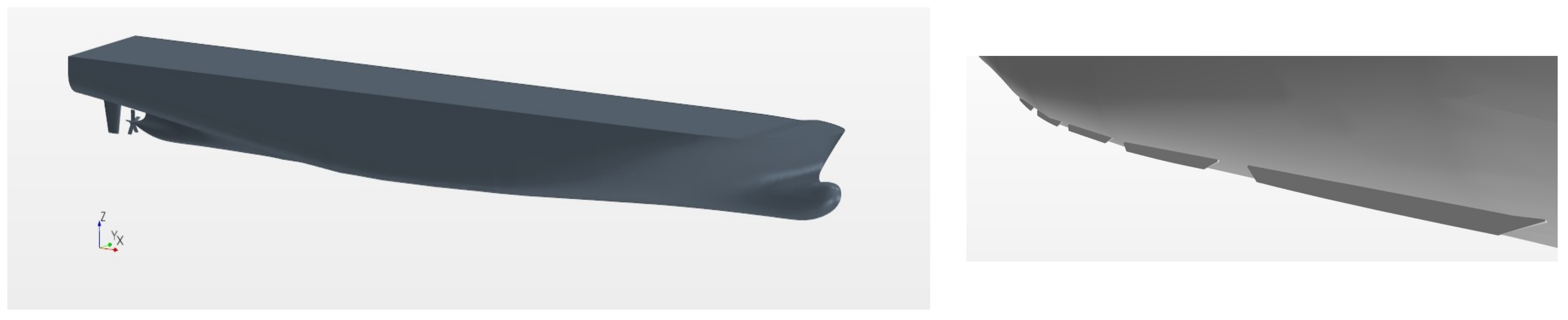
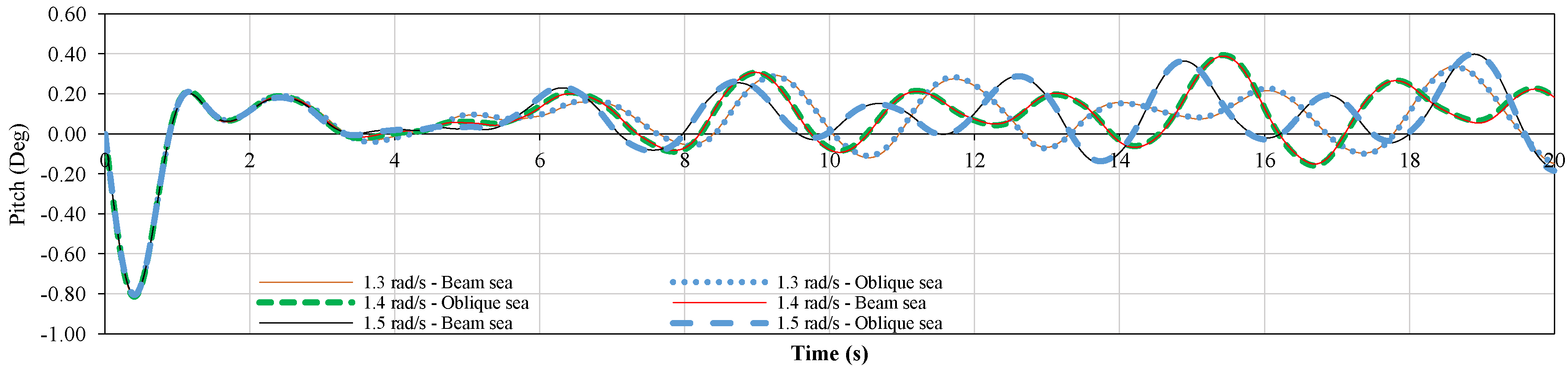
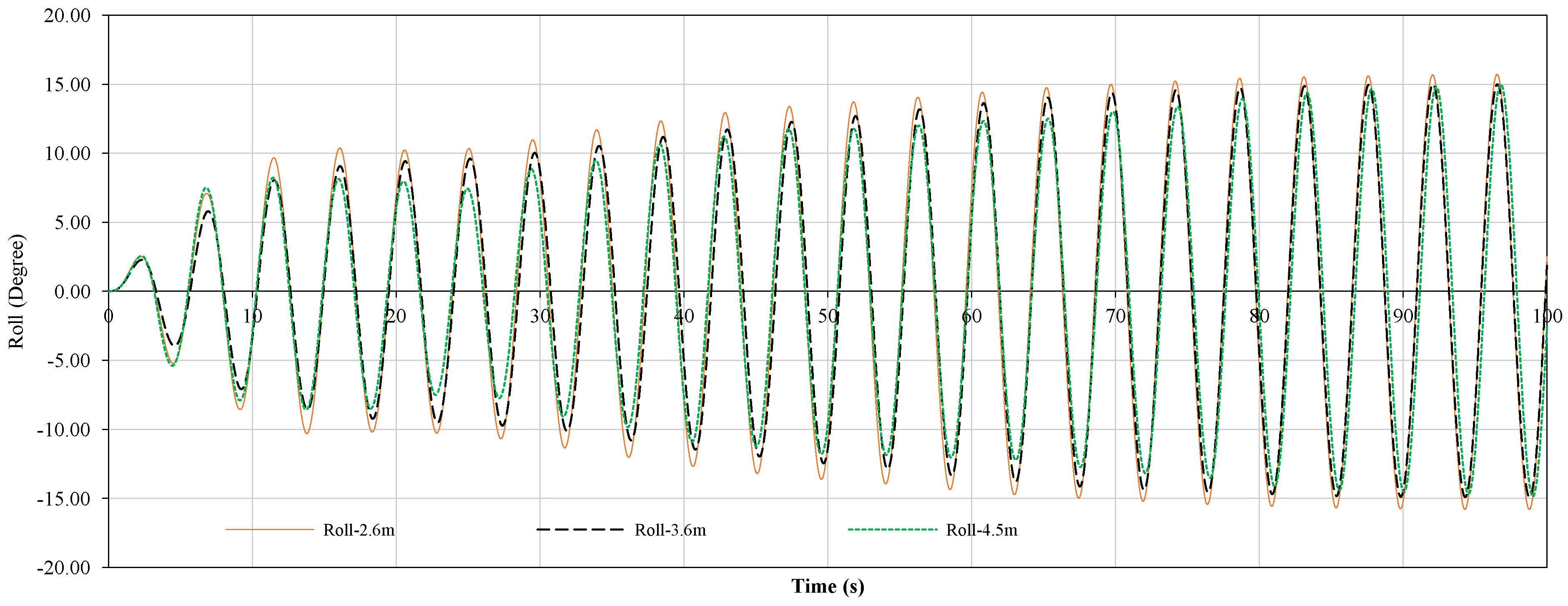
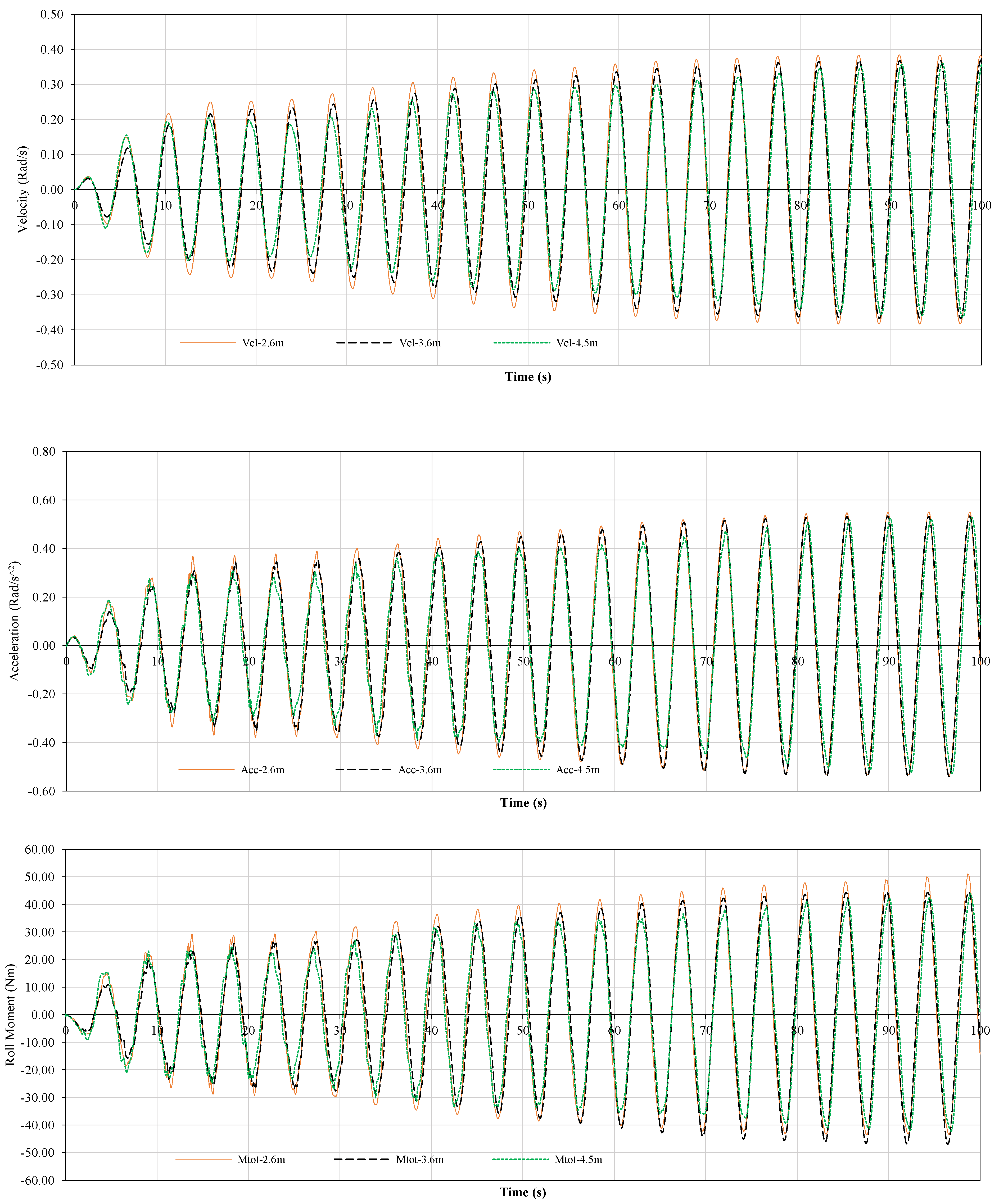
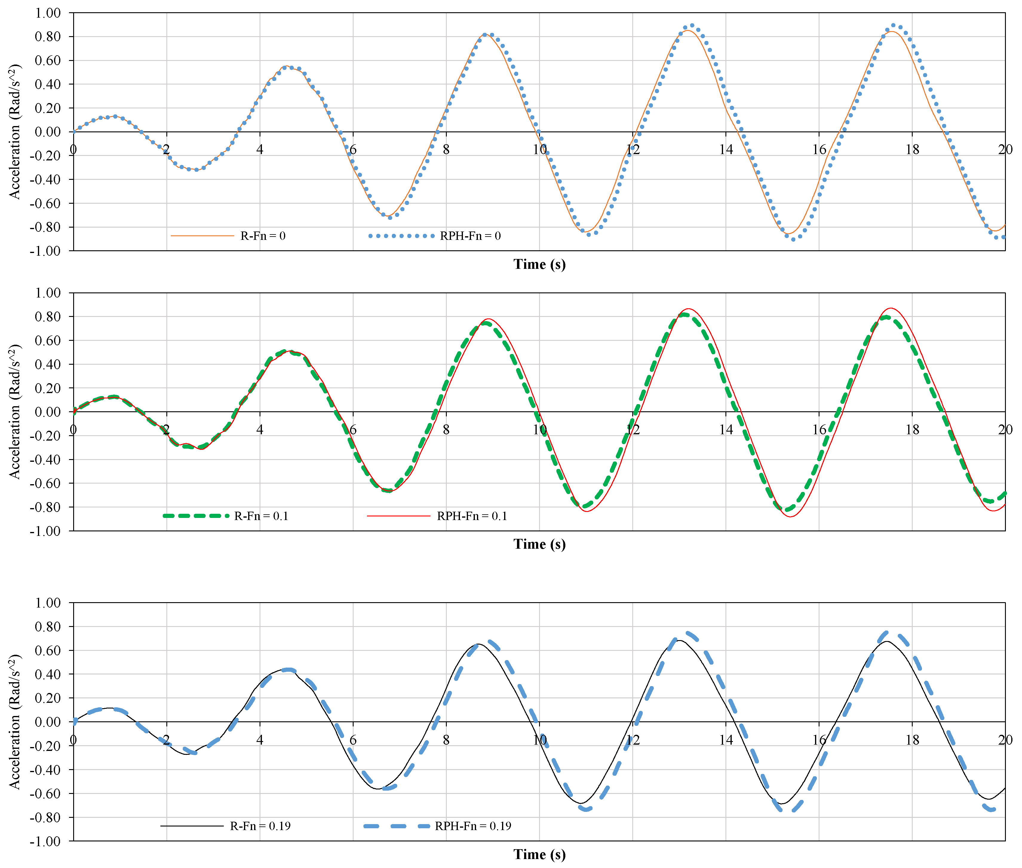
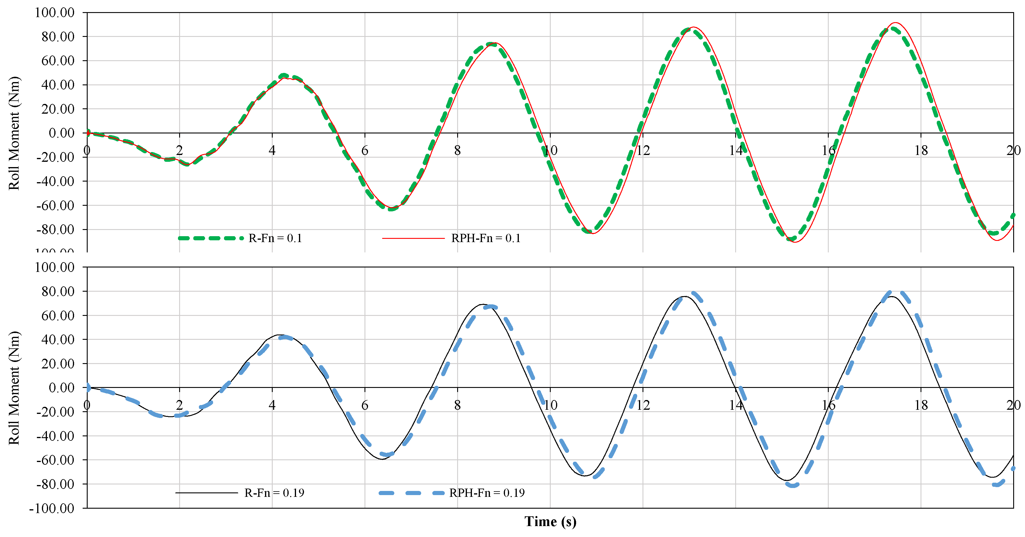
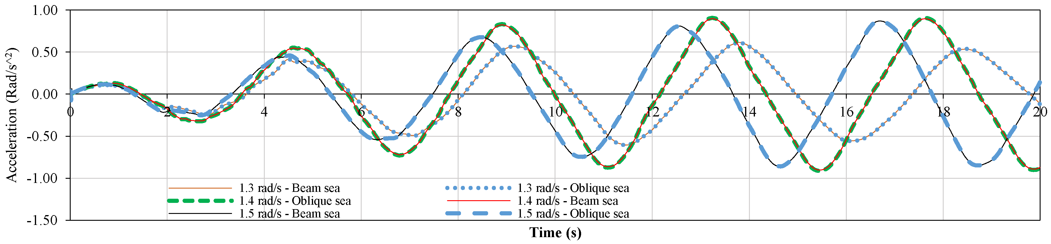
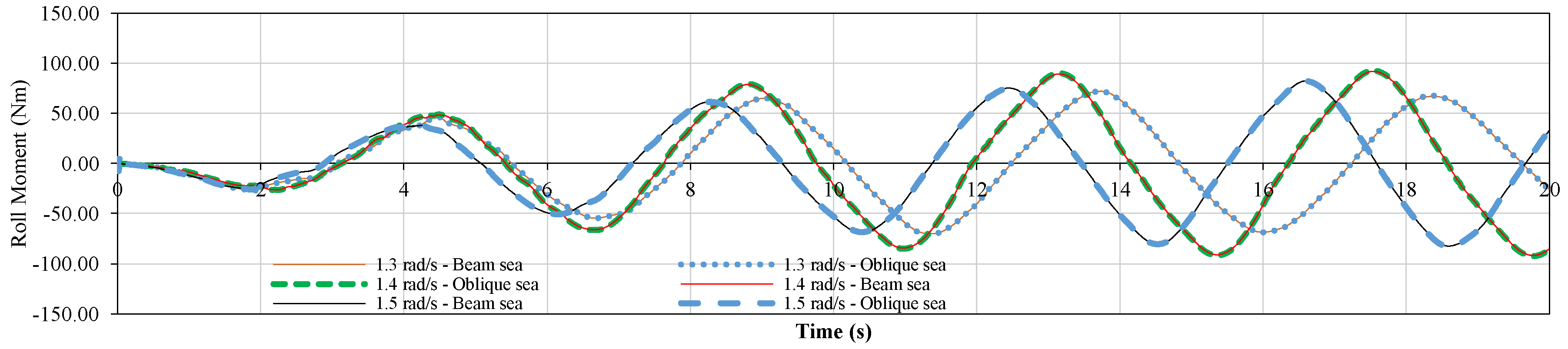
There are a limited number of studies regarding the roll damping coefficients of an entire model and most studies considered a segment of the ship especially the middle section. The focus of numerical simulations was on 2D and overlooked the effect of other motions such as pitch and longitudinal turbulence in the case with forward speed. Therefore, the impact of different degrees of freedom (DOF) on the roll damping coefficient is unknown. In the present study, the numerical simulations of a whole containership model are conducted based on the HERM technique. The impact of forward speed, DOF and excitation frequency at beam sea and oblique sea conditions on roll motion characteristics and roll damping coefficients are investigated.

2. Theoretical Background

The following discussion involves the ‘harmonic excited roll motion’ HERM technique to determine required roll damping coefficients. Regarding Blume’s experimental setup [14], the model possesses two masses at the centre of gravity that are rotating contrarily around the vertical axis. Specifically, one of the masses is rotating in a clockwise and the other is rotating in an anti-clockwise direction. The rotating mass shares the same frequency in the opposite direction to minimise the yaw motion. During contrary motion, the two masses meet at both sides of the model twice per rotation period, which imposes the maximum roll excitation moment. Various roll amplitudes can be achieved by setting different weights of the rotational masses. From the experiments [15], the amplitude of the roll exciting moment should ideally be equal to the restoring moment of the heel angle which refers to two masses of rotation on one side of the model. Originally, the equation of roll motion was formulated by using Newton’s second law is balanced between the ships’ motions and external moments as [23]:

$$[I_{44}+\delta I_{44}]\cdot \frac{d^2\phi }{d{t}^2}+N_{44}\cdot \frac{d\phi }{dt}+S_{44}\phi =F_{E44}(t)$$

(1)

whereas,

$I_{44}+\delta I_{44}$	Mass and added mass moment of inertia coefficients
$N_{44}$	Damping moment coefficient
$S_{44}$	Restoring coefficient
$F_{E44}$	Roll excitation moment

The magnitude of damping moment in roll motion is generally less than the total moment of inertia and restoring moment. However, it still is essential to estimate the damping moment because inertia and restoring moments could be shifted in 180 degrees and counteract each other. As a result, only the damping moment limits the roll motion [24]. The exciting moment changes harmonically:

$$F_{E4}(t)=F_{E44}\sin (\omega t)$$

(2)

The induced roll angle and roll velocity are as below:

$$\phi (t)={\phi }_a\sin (\omega t+\vartheta )$$

(3)

and

$$\frac{d\phi }{dt}=\stackrel{.}{\phi }(t)=\omega {\phi }_a\cos (\omega t+\vartheta )$$

(4)

The dissipated energy during a harmonic roll period is:

$$E_E=4{\displaystyle {\int }_0^{{\phi }_a}{N}_{44}\dot{\phi }d\phi }$$

(5)

Substituting the Equations (3) and (4) into Equation (5) with phase angle (𝜗 = 0) gives:

$$E_E=4{\displaystyle {\int }_0^{\frac{T}{4}}{N}_{44}\omega {\phi }_a}\cos (\omega t)\cdot \omega {\phi }_a\cos (\omega t)dt=4\cdot N_{44}{\omega }^2{\phi }_a{}^2\cdot {\displaystyle {\int }_0^{\frac{\pi }{2\omega }}{\cos }^2(\omega t)dt}$$

(6)

Allowing the general solution of the integral gives:

$${\displaystyle \int {\cos }^2(xt)dt=\frac{2xt+\sin (2xt)}{4x}}$$

(7)

The solution to define the dissipated damping energy over a cycle is:

$$E_E=4\cdot N_{44}{\omega }^2{\phi }_a{}^2\cdot {\left[\frac{2\omega t+\sin (2\omega t)}{4\omega }\right]}_0^{\frac{\pi }{2\omega }}=\pi \cdot N_{44}\omega {\phi }_a{}^2$$

(8)

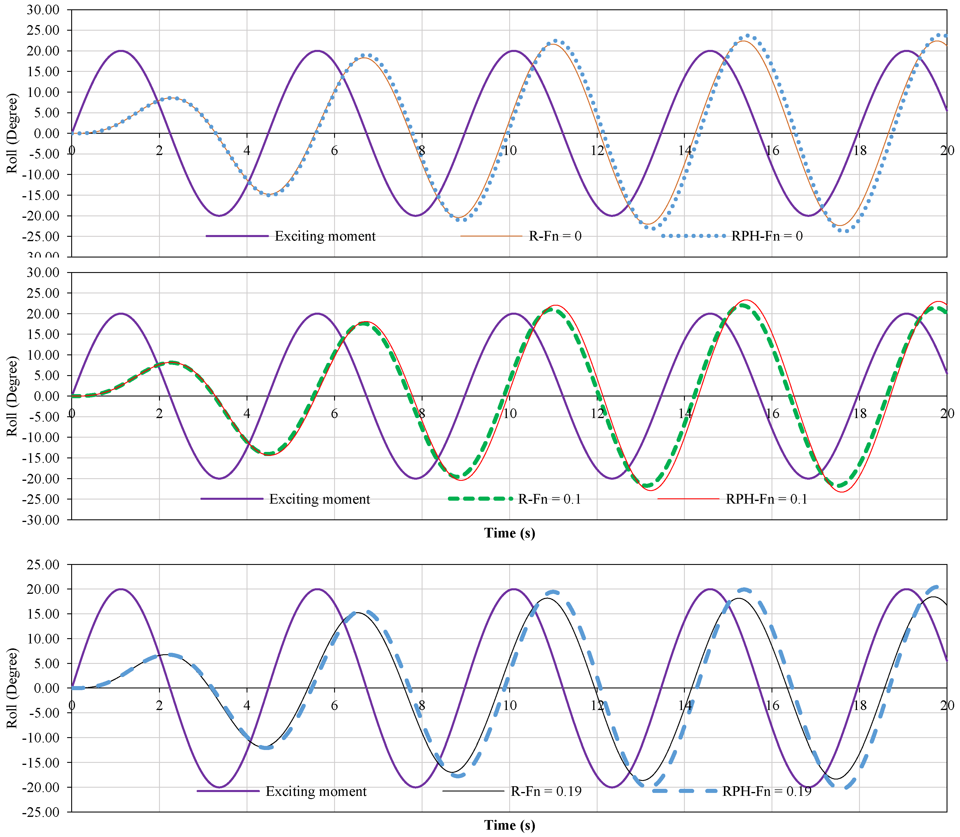
With respect to the roll moment, the roll angle is phase shifted by 𝜗. The following formula provides an estimation for the work done by the exciting moment in one roll period:

$$E_A={\displaystyle {\int }_0^T{F}_{E4}(t)\dot{\phi }(t)dt={\displaystyle {\int }_0^{\frac{2\pi }{\omega }}{F}_{E44,a}\sin (\omega t)\omega {\phi }_a\cos (\omega t+\vartheta )dt}}$$

(9)

Substituting Equation (4) into Equation (9) and after solving integral form, the formula gives:

$$E_A=F_{E44,a}{\phi }_a\pi \sin \vartheta$$

(10)

The work done by the exciting moment and the dissipated energy over one roll period should relatively be the same. There are a couple of methods available to determine the roll damping coefficient, however, this paper focuses on the relationship of 𝐸_𝐴 = 𝐸_𝐸 where the roll damping can be calculated by the following formula:

$$N_{44}=\frac{F_{E44}\sin \vartheta }{\omega {\phi }_a}$$

(11)

The damping coefficient can now be established to a dimensionless form, which was recommended by the ITTC [25].

$${\widehat{B}}_{44}=\frac{N_{44}}{\rho \nabla B_{wl}^2}\sqrt{\frac{B_{wl}}{2g}}$$

(12)

3. Model Geometry

In this study, a model of a DTC post-Panamax container ship was adopted to carry out numerical simulations. A 3D sketch of the model is shown in Figure 1. The main particulars of the model scale and the full scale are presented in

Table 1. Main Dimensions of model and full-scale ship.

Main Dimension	Full Scale (λ = 1.0)	Model Scale (λ = 59.467)
Lpp [m]	355.00	5.9697
Lwl [m]	360.91	6.0691
Bwl [m]	51.00	0.8576
D [m]	14.00	0.2354
CB [-]	0.6544	0.6544
∇ [m3]	165,868.5	0.7887
$\overline{KM}$ [m]	25.05	0.4213
$\overline{GM}$ [m]	1.37	0.023
$\overline{KG}$ [m]	23.68	0.3983
𝑇0 [s]	38.17	4.95
KXX [m]	20.25	0.340
KYY [m]	88.19	1.483
KZZ [m]	88.49	1.488

. The ship has a single screw propulsion with a five-blade arrangement and the ship’s full appendages contain a rudder and bilge keels. The base profile of the rudder consists of an NACA 0018 foil. Both port and starboard sides have five bilge keel segments that are attached symmetrically. More details about the geometry of the model and ship can be found in [15].

4. Numerical Modelling

The right numerical set up is essential to achieve a successful numerical simulation. STAR CCM+ was used to conduct the study and this section provides details of the selected approach.

4.1. Governing Equations and Physics Modelling

The solver utilizes averaged continuity and momentum equations for incompressible flow in terms of tensor and Cartesian coordinates as follows [26]:

$$\frac{\partial (\rho {\overline{u}}_i)}{\partial x_i}=0$$

(13)

$$\frac{\partial (\rho {\overline{u}}_i)}{\partial t}+\frac{\partial }{\partial x_j}(\rho {\overline{u}}_i{\overline{u}}_j+\rho \overline{u_i^{{}^{\prime }}{u}_j^{{}^{\prime }}})=-\frac{\partial \overline{p}}{\partial x_i}+\frac{\partial {\overline{\tau }}_{ij}}{\partial x_j}$$

(14)

$${\overline{\tau }}_{ij}=\mu \left(\frac{\partial {\overline{u}}_i}{\partial x_j}+\frac{\partial {\overline{u}}_j}{\partial x_i}\right)$$

(15)

The flow directions are specified by i and j indices in x and y directions. Density and viscosity of the flow are represented by ρ and μ respectively. ${\overline{u}}_i$ refers to the time-averaged velocity and $\overline{P}$ is the time-averaged pressure. The Reynolds stress tensor is illustrated by $\rho \overline{{u^{\prime }}_i{u^{\prime }}_j}$, while, ${\overline{\tau }}_{ij}$ is the mean viscous stress tensor. The selected solver is based on a finite volume approach method, which is a method for representing and evaluating partial differential equations in terms of algebraic equations. A predictor-corrector method is employed to form a relationship between continuity and momentum equations.

A turbulence model was employed due to the uncertainty of the stress tensor. In this paper, a realizable k-ε turbulence model was selected for the study. This selection decreases the simulation time in comparison to other turbulence methods such as SST and K-ω [27]. A simple multiphase approach called ‘Volume of Fluid’ (VOF) was employed to model the free surface. The mesh quality encompassing the free surface has the capability of solving interfaces between two phases. Hence, extra modelling was not necessary since the VOF method was selected. Simulations under VOF consider the same equation for a single phase or multiphase conditions, in which they also reflect the same velocity and pressure values. In order to capture the sharp interface among phases, the second order convection scheme was selected.

The solver utilizes the segregated flow model which becomes a useful tool to solve the governing equations in an uncoupled condition. Where convection terms were discretized by the second-order upwind scheme throughout the solution and the SIMMPLE algorithm was selected. To enhance the results, dynamic fluid body interaction (DFBI) method was used. This method is essential to predict the ship’s behaviour in terms of seakeeping, because the model condition is like a ship in real sea condition [28]. A courant number (CFL) method was used to define the exact time step. In order to select the time step, the CFL method and recommended time step by ITTC [29] were considered. The CFL is a proportion of a physical time step to a mesh cell dimension per mesh flow velocity (Equation (16)) and it should be kept less than one for each cell to have numerical stability. However, 0.002 seconds (T/2¹¹ (T = excitation period)) was selected as a time step for the study which is quite smaller than both methods to capture accurately the roll motion and fluid-body interaction.

$$CFL=\frac{U\Delta t}{\Delta x}$$

(16)

4.2. Meshing Structure

Overset mesh technique was used due to large motions involved in the simulations. The overset mesh does not need to any mesh modification after generating the initial mesh and the region can be transformed without remeshing, hence, it gives more flexibility and lower number of mesh [30]. This method involves two regions of overset and background. The overset region holds and surrounds the body and moves with the body while it is located inside the motionless background region. A linear interpolation method was used to taking into account the interaction between overset and background [28]. Because an overlap volumetric block was considered to generate the same cell size in both the background and overset regions at the vicinity of overset region to minimise the interpolation errors. To increase the accuracy, the overset region was refined in a more advanced mesh size and quality. This method allowed capturing boundary layer, flow separation during body motion, wave making and vortices around the body [31].

4.3. Mesh Generation

The mesh was generated according to the practical guidelines for ship CFD applications [32] and at least 40 cells per wavelength and 20 cells in the vertical direction for free surface were set. The trimmed mesher was utilised to generate a high-quality mesh and the prism layer was selected due to its capability to generate orthogonal prismatic mesh next to the body that can capture the velocity gradient and boundary layer. A surface remeshing option was used to produce a better quality of surface that can enhance volumetric mesh. For the final meshing stage, an automatic surface repair meshing tool was used to repair and purify any geometrical problems that were left over after surface remeshing. The volumetric control zones were produced around the body and in the free surface. The mesh refinement was performed mainly in these regions. Therefore, the number of cells was increased in those particular regions to capture complex flow characteristics. The cell size of the overset region and background were matched to prevent solution divergence. This was achieved by using an overlap volumetric block method. Figure 2 shows the mesh structure including the background and overset regions.

4.4. Boundary and Initial Condition

To enhance the accuracy of results, suitable initial and boundary conditions were selected (Figure 3). The inlet boundary is set one L_pp in front of the model and the outlet is located 3 L_pp after the ship. The distances of left, right and bottom boundaries from the model are one L_pp and 0.5 L_pp is chosen for the top boundary [32]. The velocity inlet and pressure outlet boundary conditions were set in a way that the stream would flow past the model in head sea condition. The initial hydrostatic pressure was selected for the outlet boundary condition to prevent any backflow. The remaining boundaries including sides, top and bottom were all set as a velocity inlet in order to prevent a velocity gradient generated from the wall and flow interactions. Therefore, these boundary settings allow the velocity flow in all lateral boundaries to be directed towards the outlet boundary with negligible flow reflection.

4.5. Coordinate System

To simulate the model’s motions, earth-fixed and body local coordinate systems were used. Initially, forces and moments on the model were calculated by analysing flow around the body. In the next step, the forces and moments were transferred into the local body coordinate where defined in the centre of gravity. The velocity and acceleration of the model were extracted from the motion’s equations and converted to the earth-fixed coordinate system. This allows detecting the new location of the model.

5. Results and Discussion

5.1. Verification Analysis

To improve the reliability of the simulation results, it is necessary to specify the level of uncertainty. Based on the verification method presented by Stern [33], the numerical uncertainty U_SN, consists of uncertainty in iterative convergence U_I, grid-spacing U_G and time-step U_T, which is formulated by the following equation:

$$U^2{}_{SN}=U^2{}_I+U^2{}_G+U^2{}_T$$

(17)

The uncertainty raised from U_I and U_T are negligible because the simulations are set in a calm water condition [34]. However, the grid-spacing uncertainty was investigated as major source of the uncertainty. Three different mesh configurations with 2.6, 3.6 and 4.5 million elements were created with a refinement ratio of r_G = $\surd 2$ which was applied mainly on overset region [27,35] and details of the generated mesh are shown in

Table 2. The number of mesh elements in different configurations.

	Background	Overset	Total
Fine (1)	2,610,127	3,604,231	4,543,826
Medium (2)	1,725,314	2,449,946	3,326,086
Coarse (3)	884,813	1,154,285	1,217,740

. The model was excited by 5.5 Nm roll exciting moment based on the HERM technique at frequencies of 1.39 rad/s which is close to the natural frequency of the model. The drag calculation at a forward speed of 1.54 m/s was performed to select a proper mesh configuration that could precisely calculate pressure and shear forces. The increment for cells mainly focussed on the overset region to refine the quality of mesh. The accuracy of the simulation results against experimental measurements specifies which mesh configuration to be selected. The initial and boundary conditions all remained constant while the number of mesh cells varied. The grid uncertainty calculation for different mesh configurations was performed based on Richardson extrapolation [34]. The variation of simulation results for cases of coarse (S₃), medium (S₂) and fine (S₁) configurations are calculated as follows:

$${\epsilon }_{G32}=S_3-S_2$$

(18)

$${\epsilon }_{G21}=S_2-S_1$$

(19)

$$R_G={\epsilon }_{G21}/{\epsilon }_{G32}$$

(20)

The numerical convergence ratio was calculated using Equation (20). Four typical conditions can be predicted for the convergence ratio: (i) monotonic convergence (0 < R_G < 1), (ii) oscillatory convergence (R_G < 0; |R_G| < 1), (iii) monotonic divergence (R_G > 1) and (iv) oscillatory divergence (R_G < 0; |R_G| > 1). For the cases (iii) and (iv) the numerical uncertainty cannot be computed. For the case (ii) uncertainty can be computed based on bounding error between upper limit S_U and lower limit S_L using Equation (21):

$$U_G=|\frac{1}{2}(S_U-S_L)|$$

(21)

In the case (i), the generalised Richardson extrapolation is adopted to compute the numerical uncertainty proposed by Stern, Wilson [36]. As the solutions were close to the asymptotic range, the correlation factor method was used to compute the numerical uncertainties. The maximum and minimum values of roll motion characteristics were taken into account to compute the uncertainty, because, the peak values are used to compute the roll damping.

The results of simulations are compared with experimental data [15] shown in

Table 3. Verification Study of numerical results versus experiments (EFD).

Amplitude	EFD	S1	S2	S3	RG	δ*REG1 (%S1)	UG (%S1)
Roll angle (°)	14.42	14.94	15.05	15.70	0.17	0.29	2.04
Roll moment (Nm)	-	43.8	44.5	50	0.13	0.47	4.42
Angular acceleration (Rad/s2)	-	0.528	0.532	0.549	0.24	0.47	2.18
Angular velocity (Rad/s)	-	0.362	0.368	0.382	0.43	2.49	5.25
Drag (N)	26.46	27.9	28.14	30.5	0.10	0.19	2.36

and the roll motion characteristics for a couple of cycles are shown in Figure 4. The numerical simulations were performed at 6DOF similar to experimental tests. Overall, the simulation results have produced larger values than experimental values. The verification study shows that the uncertainty value is small and about 5 for the worst condition. It was found that the 4.5 million mesh cells produce the most reliable results and could achieve the closest value to the experimental data. The maximum roll angle and drag have a 4.02% and 5.44% difference with experimental measurements, respectively. This numerical approach has the ability to simulate roll motion accurately. Hence, it was used to simulate roll motion characteristics in different conditions. In this study, a maximum of 3DOF (RHP) was considered for investigating dynamic stability according to the most popular equation methods, which have three degrees of freedom. Decreasing the number of degrees of freedom reduces the maximum roll angle because the moment of inertia and restoring moment do not fully counteract each other. Therefore, the computed roll damping moment, based on Handschel’s method, is overestimated and using the proposed method in Section 5.4 can compute the roll damping coefficients more accurately.

5.2. Influence of Forward Speed and DOF

The roll damping coefficient cannot be computed directly from numerical simulations and requires time series analysis. Therefore, prior to discussing the damping coefficient, the influence of forward speed, degrees of freedom (DOF), different frequencies, beam sea and oblique sea conditions are studied. The model was excited based on the HERM technique at different conditions as presented in

Table 4. Test conditions to study the impact of forward speed, DOF, excitation frequency, beam and oblique sea on roll motion and damping coefficients.

Case No.	Fn.	Frequency (Rad/s)	DOF	Sea Condition	Roll Exciting Moment (Nm)	Pitch Exciting Moment (Nm)
1	0	1.4	R	Beam sea	20	-
2	0	1.4	RHP	Beam sea	20	-
3	0.1	1.4	R	Beam sea	20	-
4	0.1	1.4	RHP	Beam sea	20	-
5	0.19	1.4	R	Beam sea	20	-
6	0.19	1.4	RHP	Beam sea	20	-
7	0	1.3	RHP	Beam sea	20	-
8	0	1.5	RHP	Beam sea	20	-
9	0	1.3	RHP	Oblique sea	20	10
10	0	1.4	RHP	Oblique sea	20	10
11	0	1.5	RHP	Oblique sea	20	10

. In order to investigate the impact of DOF on roll motion characteristics, two conditions were considered (a) model free in just roll motion and restrain in other 5 DOF, (b) the model free in roll, heave and pitch (RHP) and restrain in surge, sway and yaw. Three different Froude numbers of 0, 0.1 and 0.19 were selected to investigate the impact of forward speed. In order to keep the results consistent, the physical simulation times were set to 20 s. The harmonic excited roll motion was generated from the beginning (zero degrees) and continued until the physical time of 20 s to demonstrate the motions of the model similar to real sea condition. This method enhances the accuracy of the motions for a better analysis. The changes of roll, angular velocity, angular acceleration and roll moment are shown in Figure 5, Figure 6, Figure 7 and Figure 8. By observing the first two cycles of the plots, the model tends to absorb energy from the roll exciting moment in terms of the moment of inertia. Therefore, the roll motion characteristics increase gradually and remain constant in the following cycles. Decreasing the DOF to roll motion slightly decreases the amplitude of motion characteristics and the reduction is significant at higher Froude numbers. At zero forward speed, the roll angle difference between R and RHP conditions is 1.4 degrees, while the difference is 2.1 degrees at Froude number 0.19. Increasing the DOF increases the phase shift between the roll exciting moment and roll time trace (Figure 5). However, increasing the forward speed reduces the phase shift, because added dynamic pressure speeds up the rolling motion of the model. The angular velocity is a function of the roll time trace and a similar trend is observed. Increasing the forward speed and reducing the DOF reduce the amplitude of angular velocity (Figure 6). The model free in RHP at zero forward speed experiences higher angular acceleration and roll moment, whereas, the model free in just roll motion with the highest Froude number experiences lower angular acceleration and roll moment.

5.3. Influence of Excitation Frequency and Heading

The model was excited in both beam sea and oblique sea conditions at different excitation frequencies including 1.3, 1.4 and 1.5 rad/s to investigate the effects of frequency and exciting moment direction on the roll motion characteristics. The variation of roll, angular velocity, angular acceleration, roll moment and pitch angle are shown in Figure 9, Figure 10, Figure 11, Figure 12 and Figure 13. For the beam sea condition, 20 Nm roll exciting moment was applied on the model, while, for the oblique sea condition, 20 Nm and 10 Nm of roll and pitch exciting moment simultaneously were applied on the model respectively. The roll motion characteristics of the oblique sea conditions are slightly larger than the beam sea condition at various frequencies, although the total exciting moment in oblique condition is considerably larger. Because the model is more stable in longitudinal section and 10 Nm pitch exciting moment has negligible effects on pitch and roll motions. The model generates larger roll motion characteristics at a frequency of 1.4 rad/s which is close to the natural frequency of the model. The model achieves a 24-degree roll angle at 1.4 rad/s larger than 20.5 and 18 degrees for the frequency of 1.5 and 1.3 rad/s. At the resonance frequency, the induced moment of inertia and restoring moment have the same magnitude in the opposite direction hence counteracting each other. As a result, the damping moment which is not large resists the development of roll motion and the exciting moment imposes the model towards a larger roll angle. The angular velocity and roll moment of the model at a frequency of 1.4 rad/s is also larger than other frequencies, similar to the roll angle which is larger than the other two. However, the induced angular acceleration in the case of 1.5 rad/s is as large as the case of 1.4 rad/s. That is due to being located in the region dominated by acceleration where the magnitude of acceleration for the same amplitude of roll angle is larger compared to a lower range of frequency. The pitch angle changes with regard to the change of roll angle. The model experiences forward trim, because the wetted surface area and water pressure of the aft half of the model is larger than the forward half. The pitch angle at a frequency of 1.4 rad/s is larger due to a larger roll angle.

5.4. Roll Damping Coefficient

The dimensionless damping coefficients of the model in different conditions are presented in

Table 5. Non-dimensional roll damping of the model at different cases.

Case No.	Maximum Roll Angle (Degrees)	Difference IN & RE (N)	Amplitude of Exciting Moment (N)	Phase Shift (Rad)	Dimensionless Damping Coefficient (CFD)	Dimensionless Damping Coefficient (EFD.)
1	22.39	11.17	8.83	0.98	0.004816	0.00462
2	23.94	11.077	8.93	1.11	0.004907	0.00482
3	21.47	10.257	9.75	0.93	0.00535	-
4	22.98	10.11	9.89	1.02	0.00541	-
5	18.46	10.82	9.19	0.86	0.00553	-
6	20.48	10.57	9.44	1.01	0.00571	-
7	18.12	12.09	7.91	0.58	0.00377	0.00384
8	20.92	7.43	12.57	1.5	0.00822	0.00431
9	18.15	12.15	7.75	0.59	0.00376	-
10	24.18	11.14	8.86	1.11	0.00483	-
11	20.98	7.59	12.41	1.5	0.00809	-

. The damping coefficients were extracted from roll motion characteristics based on Equation (11) and were converted into a dimensionless number, which was recommended by the ITTC [25]. The model was free up to 3DOF and was excited at frequencies higher and lower than the natural frequency. Hence, the maximum roll motion characteristics were decreased compared to 6DOF at resonance conditions. That is because the total moment of inertia (IN) and restoring moment (RE) cannot counteract each other completely. The restoring moment was calculated by Autohydro software and the virtual moment of inertia was calculated based on [37]. The roll exciting moment compensates the difference between these two. Therefore, the amplitude of the real roll exciting moment decreases during a cycle.

It can be seen from cases 1 to 6 that reducing the DOF number at different Froude numbers reduces the maximum roll, whereas the damping coefficient relatively slightly increases (compared to the experimental values). The rudder angle was set at zero during the simulation to avoid any effect on extracting the damping coefficient. Increasing the forward speed increases the magnitude of the damping coefficient due to changes in pressure distribution around the model. However, the pressure variations are small and by reduction of the maximum roll angle, the damping coefficient increases. The damping coefficients of cases 1 and 2 are in acceptable agreement with existing results from the model tests [15]. Changing the excitation frequency changes the roll motion specifications and the damping coefficient. At frequencies of 1.3 rad/s (case 7) and 1.4 rad/s (case 2) the extracted damping coefficients are in good agreement compared to the experimental data, while for the frequency of 1.5 rad/s which is higher than the natural frequency the result is overestimated. Because, the energy conservation method to extract damping coefficient works well for frequencies equal or smaller than natural frequency of the model. For higher range of frequencies, the computed roll damping is overestimated because of the larger phase shift between roll exciting moment and roll angle, as well as smaller difference between virtual moment of inertia and restoring moment. This means the energy conservation method works at a range of frequency lower and close to the natural frequency. As discussed in the previous section, the roll motion characteristics in oblique sea condition are slightly larger than beam sea condition, while the computed damping coefficients of oblique sea condition are slightly smaller than the beam sea condition.

6. Conclusions

Numerical simulations based on the HERM technique were carried out to investigate the influence of excitation frequency, Froude number, DOF and the model’s heading on roll motion and roll damping coefficients. If the model is free in just roll motion, it experiences smaller motion characteristics compared to the model free in coupled roll-pitch-heave motions. However, the reduction with a higher Froude number is more. Nevertheless, the model free in roll motion has relatively a larger roll damping coefficient at different forward speeds. The applied energy conservation method to calculate the damping moment is valid at a low range of frequencies as well as the natural frequency. The model under the same roll exciting moment in beam sea and oblique sea conditions generates similar roll motion and roll damping coefficients. The findings of this study improve the equation base methods to advance prediction of roll motion and to investigate the dynamic stability of a ship.

References

1. Ikeda, Y.; Himeno, Y.; Tanaka, N. A Prediction Method for Ship Roll Damping; Department of Naval Architecture, University of Osaka Prefecture: Osaka, Japan, 1978. [Google Scholar]
2. Gu, M.; Lu, J.; Wang, T. Experimental and numerical study on stability under dead ship condition of a tumblehome hull. In Proceedings of the 13th International Ship Stability Workshop, Brest, France, 23–26 September 2013. [Google Scholar]
3. Bass, D.; Haddara, M. Nonlinear models of ship roll damping. Int. Shipbuild. Prog. 1988, 35, 5–24. [Google Scholar]
4. Roddier, D.; Liao, S.-W.; Yeung, R. Wave-induced motion of floating cylinders fitted with bilge keels. Int. J. Offshore Polar Eng. 2000, 10, 241–248. [Google Scholar]
5. Na, J.H.; Lee, W.C.; Shin, H.S.; Park, I.K. A design of bilge keels for harsh environment FPSOs. In Proceedings of the Twelfth International Offshore and Polar Engineering Conference, Kitakyushu, Japan, 26–31 May 2002. [Google Scholar]
6. Jung, K.H.; Chang, K.-A.; Huang, E.T. Two-dimensional flow characteristics of wave interactions with a free-rolling rectangular structure. Ocean Eng. 2005, 32, 1–20. [Google Scholar] [CrossRef]
7. Yi-Hsiang, Y.; Kinnas, S.A.; Vinayan, V.; Kacham, B.K. Modeling of flow around FPSO hull sections subject to roll motions: Effect of the separated flow around bilge keels. In Proceedings of the Fifteenth International Offshore and Polar Engineering Conference, Seoul, Korea, 19–24 June 2005. [Google Scholar]
8. Kinnas, S.A.; Yi-Hsiang, Y.; Vinayan, V. Prediction of flows around FPSO hull sections in roll using an unsteady Navier-Stokes solver. In Proceedings of the Sixteenth International Offshore and Polar Engineering Conference, San Francisco, CA, USA, 28 May–2 June 2006. [Google Scholar]
9. Wilson, R.V.; Carrica, P.M.; Stern, F. Unsteady RANS method for ship motions with application to roll for a surface combatant. Comput. Fluids 2006, 35, 501–524. [Google Scholar] [CrossRef]
10. Yu, Y.-H.; Kinnas, S.A. Roll response of various hull sectional shapes using a Navier-Stokes solver. J. Offshore Polar Eng. 2009, 19, 46–51. [Google Scholar]
11. Bangun, E.; Wang, C.; Utsunomiya, T. Hydrodynamic forces on a rolling barge with bilge keels. Appl. Ocean Res. 2010, 32, 219–232. [Google Scholar] [CrossRef]
12. Thiagarajan, K.P.; Braddock, E.C. Influence of bilge keel width on the roll damping of FPSO. J. Offshore Polar Eng. 2010, 132, 011303. [Google Scholar] [CrossRef]
13. Avalos, G.O.; Wanderley, J.B.; Fernandes, A.C.; Oliveira, A.C. Roll damping decay of a FPSO with bilge keel. Ocean Eng. 2014, 87, 111–120. [Google Scholar] [CrossRef]
14. Blume, P. Experimentelle Bestimmung von Koeffizienten der wirksamen Rolldämpfung und ihre Anwendung zur Abschätzung extremer Rollwinkel. Schiffstechnik 1979, 26, 3–23. [Google Scholar]
15. Handschel, S.; Abdel-Maksoud, M. Improvement of the Harmonic Excited Roll Motion Technique for Estimating Roll Damping. Ship Technol. Res. 2014, 61, 116–130. [Google Scholar] [CrossRef]
16. Begovic, E.; Day, A.H.; Incecik, A.; Mancini, S.; Pizzirusso, D. Roll damping assessment of intact and damaged ship by CFD and EFD methods. In Proceedings of the 12th international conference on the stability of ships and ocean vehicles, Glasgow, UK, 13–19 June 2015; pp. 14–19. [Google Scholar]
17. Mancini, S.; Begovic, E.; Day, A.H.; Incecik, A. Verification and validation of numerical modelling of DTMB 5415 roll decay. Ocean Eng. 2018, 162, 209–223. [Google Scholar] [CrossRef]
18. Zhou, Y.-h.; Ning, M.; Xun, S.; ZHANG, C. Direct calculation method of roll damping based on three-dimensional CFD approach. J. Hydrodyn. Ser. B 2015, 27, 176–186. [Google Scholar] [CrossRef]
19. Somayajula, A.; Falzarano, J. Application of advanced system identification technique to extract roll damping from model tests in order to accurately predict roll motions. Appl. Ocean Res. 2017, 67, 125–135. [Google Scholar] [CrossRef]
20. Irkal, M.A.; Nallayarasu, S.; Bhattacharyya, S. CFD approach to roll damping of ship with bilge keel with experimental validation. Appl. Ocean Res. 2016, 55, 1–17. [Google Scholar] [CrossRef]
21. Wassermann, S.; Feder, D.-F.; Abdel-Maksoud, M. Estimation of ship roll damping—A comparison of the decay and the harmonic excited roll motion technique for a post panamax container ship. Ocean Eng. 2016, 120, 371–382. [Google Scholar] [CrossRef]
22. Oliva-Remola, A.; Bulian, G.; Pérez-Rojas, L. Estimation of damping through internally excited roll tests. Ocean Eng. 2018, 160, 490–506. [Google Scholar] [CrossRef]
23. Enshaei, S.S.K. Quantifying Ship’s Dynamic Stability through Numerical Investigation of Weight Distribution. In Proceedings of the 13th International Conference on the Stability of Ships and Ocean Vehicles (STAB), Kobe, Japan, 16–21 September 2018. [Google Scholar]
24. Kianejad, S.S.; Duffy, J.; Ansarifard, N.; Ranmuthugala, D. Ship Roll Damping Coefficient Prediction Using CFD. In Proceedings of the 32nd Symposium on Naval Hydrodynamics, Hamburge, Germany, 5–10 August 2018. [Google Scholar]
25. Reed, A.; Reed, A.M. 26th ITT C parametric roll benchmark study. In Proceedings of the 12th International Ship Stability Workshop, Washington, DC, USA, 2011. [Google Scholar]
26. Ferziger, J.H.; Peric, M.; Leonard, A. Computational Methods for Fluid Dynamics; American Institute of Physics (AIP): College Park, MD, USA, 1997. [Google Scholar]
27. Tezdogan, T.; Demirel, Y.K.; Kellett, P.; Khorasanchi, M.; Incecik, A.; Turan, O. Full-scale unsteady RANS CFD simulations of ship behaviour and performance in head seas due to slow steaming. Ocean Eng. 2015, 97, 186–206. [Google Scholar] [CrossRef]
28. CD-adapco, S. STAR CCM+ User Guide Version 12.04; CD-Adapco: New York, NY, USA, 2017. [Google Scholar]
29. ITTC. Guidelines: Practical Guidelines for Ship CFD Applications; Lyngby, Denmark, 2011; pp. 1–18. [Google Scholar]
30. Kianejad, S.S.; Duffy, J.; Ansarifard, N. Calculation of Restoring Moment in Ship roll motion through Numerical Simulation. In Proceedings of the 13th Int. Conference on the Stability of Ships and Ocean Vehicles (STAB), Kobe, Japan, 16–21 September 2018. [Google Scholar]
31. Field, P.L. Comparison of RANS and Potential Flow Force Computations for the ONR Tumblehome Hullfrom in Vertical Plane Radiation and Diffraction Problems; Virginia Tech: Blacksburg, VA, USA, 2013. [Google Scholar]
32. Procedures, I.-R. Practical Guidelines for Ship CFD Applications. In Guidelines 2011; 26th ITTC Specialist Committee on CFD in Marine Hydrodynamics; Lyngby, Denmark, 2011; pp. 1–18. [Google Scholar]
33. Stern, F.; Wilson, R.V.; Coleman, H.W.; Paterson, E.G. Comprehensive approach to verification and validation of CFD simulations-Part 1: Methodology and procedures. Trans. Am. Soc. Mech. Eng. J. Fluids Eng. 2001, 123, 793–802. [Google Scholar] [CrossRef]
34. Jin, Y.; Chai, S.; Duffy, J.; Chin, C.; Bose, N.; Templeton, C. RANS prediction of FLNG-LNG hydrodynamic interactions in steady current. Appl. Ocean Res. 2016, 60, 141–154. [Google Scholar] [CrossRef]
35. Tezdogan, T.; Incecik, A.; Turan, O. Full-scale unsteady RANS simulations of vertical ship motions in shallow water. Ocean Eng. 2016, 123, 131–145. [Google Scholar] [CrossRef]
36. Stern, F.; Wilson, R.; Shao, J. Quantitative V&V of CFD simulations and certification of CFD codes. Int. J. Numer. Methods Fluids 2006, 50, 1335–1355. [Google Scholar]
37. Kianejad, S.; Enshaei, H.; Ranmuthugala, D. Estimation of added mass moment of inertia in roll motion through numerical simulation. In Proceedings of the PACIFIC 2017 International Maritime Conference, Sydney, Australia, 3–5 October 2017; pp. 1–15. [Google Scholar]
Figure 1. A 3D geometry of the model and bilge keels set up at midsection.
Jmse 06 00101 g001
Figure 2. A 3D illustration of computational mesh.
Jmse 06 00101 g002
Figure 3. A 2D illustration of the overset and background regions with the applied boundary conditions.
Jmse 06 00101 g003
Figure 4. Influence of different mesh configurations on roll angle, angular roll velocity, angular roll acceleration and roll moment under 5.5 Nm roll exciting moment at frequency of 1.39 rad/s with zero forward speed and 6DOF.
Jmse 06 00101 g004aJmse 06 00101 g004b
Figure 5. Roll angle time trace of the model under 20 Nm exciting moment at frequency of 1.4 rad/s, Fn = 0, Fn = 0.1, Fn = 0.19 and considering different degrees of freedom. Roll, heave and pitch motions are shown by R, H and P, respectively.
Jmse 06 00101 g005
Figure 6. Angular roll velocity (Vel.) time trace of the model under 20 Nm exciting moment at frequency of 1.4 rad/s, Fn = 0, Fn = 0.1, Fn = 0.19 and considering different degrees of freedom. Roll, heave and pitch motions are shown by R, H and P, respectively.
Jmse 06 00101 g006aJmse 06 00101 g006b
Figure 7. Angular roll acceleration (Acc.) time trace of the bare hull model under 20 Nm exciting moment at frequency of 1.4 rad/s, Fn = 0, Fn = 0.1, Fn = 0.19 and considering different degrees of freedom. Roll, heave and pitch motions are shown by R, H and P, respectively.
Jmse 06 00101 g007
Figure 8. Total roll moment (Mtot) time trace of the model under 20 Nm exciting moment at frequency of 1.4 rad/s, Fn = 0, Fn = 0.1, Fn = 0.19 and considering different degrees of freedom. Roll, heave and pitch motions are shown by R, H and P, respectively.
Jmse 06 00101 g008aJmse 06 00101 g008b
Figure 9. Roll angle time trace of the model under 20 Nm roll exciting moment at the frequencies of 1.3, 1.4 and 1.5 rad/s, Fn = 0 and considering beam sea and oblique sea conditions.
Jmse 06 00101 g009
Figure 10. Angular roll velocity time trace of the model under 20 Nm roll exciting moment at the frequencies of 1.3, 1.4 and 1.5 rad/s, Fn = 0 and considering beam sea and oblique sea conditions.
Jmse 06 00101 g010
Figure 11. Angular roll acceleration time trace of the model under 20 Nm roll exciting moment at the frequencies of 1.3, 1.4 and 1.5 rad/s, Fn = 0 and considering beam sea and oblique sea conditions.
Jmse 06 00101 g011
Figure 12. Total roll moment time trace of the model under 20 Nm roll exciting moment at the frequencies of 1.3, 1.4 and 1.5 rad/s, Fn = 0 and considering beam sea and oblique sea conditions.
Jmse 06 00101 g012
Figure 13. Pitch angle time trace of the model under 20 Nm roll exciting moment at the frequencies of 1.3, 1.4 and 1.5 rad/s, Fn = 0 and considering beam sea and oblique sea conditions.
Jmse 06 00101 g013