1. Introduction
Real ocean waves can be described as a superposition of many sinusoidal waves with different wavelengths, amplitudes, initial phases and propagation directions, by assuming that the wave process is stationary. They are represented by adopting two widely used wave spectrum models namely Pierson-Moskowitz (P-M) and Joint North Sea Wave Project (JONSWAP), respectively [
1,
2]. The P-M spectrum model is based on long-term observations of the wave fields in the North Sea [
1]. On the other hand, JONSWAP spectrum model is based on the observations obtained along a profile in the North Sea westward from the Sylt Island (Westerland, Germany). JONSWAP spectrum in comparison with the P-M spectrum has an advantage including the effect of limited wind fetch and water depth [
2]. Furthermore, in terms of a wave spectrum, the wave-wave interactions can be formulated, according to Hasselmann [
3].
As known, there are some waves in the ocean that resemble what is considered to be a superimposition of sinusoidal waves. Severe waves, generated by a distant storm, tsunami or solitary waves, are some examples. Such waves can be surprisingly regular, but never pure sine waves. Behind the common reference to the “random” sea state, there are other models of sea surface in which the full description of the surface motion is approximated by different mathematical formulations. Among them, a very powerful tool is represented by bichromatic wave group of full modulation. The main characteristics of such multi-component wave patterns, constituted by two superimposed sinusoidal waves, are:
the envelope travels unchanged;
each component travels with its own phase velocity, in accordance with the dispersion relation.
The model is a simple but effective way to analyze the beat pattern, also known as wave group, as well as the generation of Low Frequency Waves (LFWs). Such waves are important not only for the additional wave induced velocity and long wave effect on the short wave hydrodynamics [
4,
5], but also for the formation of standing waves, or a cross-shore and longshore nodal structure (e.g., Holman and Bowen [
6]). Bichromatic wave groups, in fact, were used in laboratory work specifically focused on surf-beat-generation mechanisms [
7,
8] or on breakpoint modulation [
9,
10,
11]. More recently, cross-shore long wave generation on relatively steep (1:10) and mild (1:40) slopes were studied by Dong [
12]. The breakpoint forced long waves were observed primarily on the steep slope, also according to Baldock et al. [
13], for which much of the incident wave grouping remains within the swash zone and at the still water shoreline. Furthermore, at the incident wave group frequency, the shoreline motion is modulated. They also found that the swash oscillations, driven by the bichromatic wave groups on the 1:10 slope, are largely dominated by low-frequency motions.
On the other hand, for a mild slope beach, Dong [
12] found that the released bound long waves are the major contributors to the free long waves. This is clearly in line with the conclusion drawn by Madsen et al. [
14,
15] in discussing surf beat and swash oscillations induced by bichromatic wave groups and irregular waves on gentle beach slopes using a Boussinesq-type wave model. According to their findings, the shoreline motion consists of a significant low-frequency component at the group frequency and individual swash of the primary waves.
Padilla and Alsina [
16] investigated the influence of the frequency bandwidth on the propagation of bichromatic wave groups over a constant 1:100 beach slope. The authors found that in the low frequency domain a larger growth of the incident bound long wave for broad band wave conditions is detected.
Numerical modeling [
17,
18] has been used to investigate the role of surf beat. In particular, long wave terms were included and excluded from a numerical model and the predicted morphology compared with a measured beach profile related to random wave tests. Therefore, considering long waves in the model, the results showed a smoothed bar, reduced bar height and moved bar crest seaward, and also less erosion in the inner surf zone. Jannat and Asano [
19] adapted a numerical model from Kobayashi et al. [
20] to investigate sediment transport under long waves. The long waves induced small changes in the surf zone, and larger changes in the Swash Zone (SZ), where long waves have maximum amplitude. According to Halfiani and Ramli [
21], numerical results on the deformation of bichromatic wave groups based on the third order side band solution of Benjamin-Bona-Mahony equation showed that nonlinear effects determine deformation of the wave groups.
Both free and forced long waves occur in the nearshore zone and surf zone, but little previous work has examined the overall impact of free long waves on the beach evolution. Similarly, direct study of how sediment transport and the erosion or accretion of beaches are influenced and modified by long waves and wave groups is still lacking. In fact, although there have been many investigations on the kinematics of extreme waves in deep water using focused wave groups in wave flumes and basins [
22,
23,
24,
25,
26], there has been little research on the wave grouping in the nearshore environment [
27,
28]. For repeated wave groups, Borthwick et al. [
29] confirm the presence of a low frequency free wave, followed by higher frequency waves of the main group and trailing higher order harmonic waves.
Under random wave conditions in small-scale experiments, Dally [
30] observed that seiching influences the final equilibrium profile, smooths the bar-trough morphology and carries sediment higher in the swash zone.
Both bichromatic and random (JONSWAP) waves were used by Brocchini and Bellotti [
31] to evaluate and simplify a theoretical model of Shoreline Boundary Conditions to be used as the SZ boundary in wave-averaged nearshore circulation models. Although there are insights about the effects of individual long-waves in hydrodynamic and shoreline motion terms, few direct experiments have investigated the influence of free long waves and wave groups on surf and swash zone morphodynamics. Their influence appears significant, as shown by Baldock et al. [
32,
33], with free long waves tending to reduce offshore sediment transport or increase onshore sediment transport. On the other hand, bichromatic wave groups resulted in much greater erosion than equivalent monochromatic waves. Furthermore, the small-scale of the experiments (water depth 0.5 m, wave height 0.05 m–0.1 m) meant that scale-effects could have been significant in influencing the results. The complexity of the problem suggested the need to obtain and operate on data acquired through laboratory investigations at a larger scale. The present study is based on high quality data from tests carried out in a large wave flume, as part of the SUSCO (Swash zone response Under grouping Storm Conditions) experiment within the Hydralab III program [
34]. The scale of experiment is arbitrary. Froude similarity is normally considered in open-channel hydraulics, where friction effects are negligible. However, in movable bed experiments, the scaling law should take into account the size of model sediments. In particular, a scaling law related to the dimensionless fall velocity must be considered. Scale effects are always present but are minimized by using a large wave flume.
The main aim is to investigate swash zone under storm conditions. A low frequencies analysis under bichromatic and monochromatic wave conditions has led to important considerations on resonant interactions detected in the wave flume and related to swash zone hydrodynamics.
2. Model Setup and Experimental Program
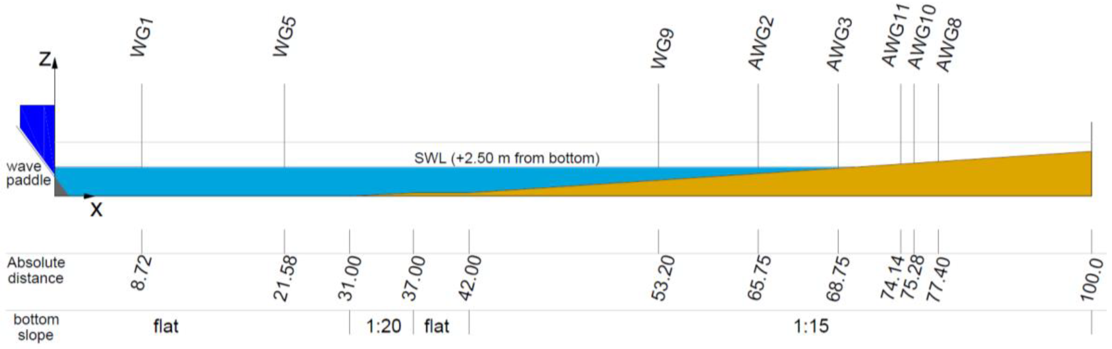
The tests were carried out at the Universitat Politècnica de Catalunya (UPC) in the Canal d’Investigació i Experimentació Marítima (CIEM) large-scale wave flume. The facility has a water depth at the toe of the paddle of about 2.5 m, a length of 100 m and a width of 3 m. The medium sediment size and measured sediment fall velocity were 0.25 mm and 34 mm/s, respectively.
Considering a horizontal coordinate (x) moving from the wave paddle toward the shoreline, the sandy beach profile consisted of the following sections (
Figure 1):
from x = 31 to 37 m, a 1:20 slope plane beach;
from x = 37 to 42 m, a plane bed;
from x = 42 to 100 m, an overall mean beach gradient of approximately 1:15.
The profile represents a sand beach in the UPC wave flume that has been investigated previously (e.g., [
11,
35]). In particular, the 1:15 slope of the inner surf and swash zone were deliberately chosen to be far enough from an equilibrium profile, taking into account underlying beach conditions and tested sea states. It is worth noting that the slope represents the theoretical limit between steep and moderate beaches and, therefore, represents a transient swash regime. Such beach slope, moreover, has been investigated by several laboratories [
36,
37,
38,
39] and field studies (e.g., [
40]).
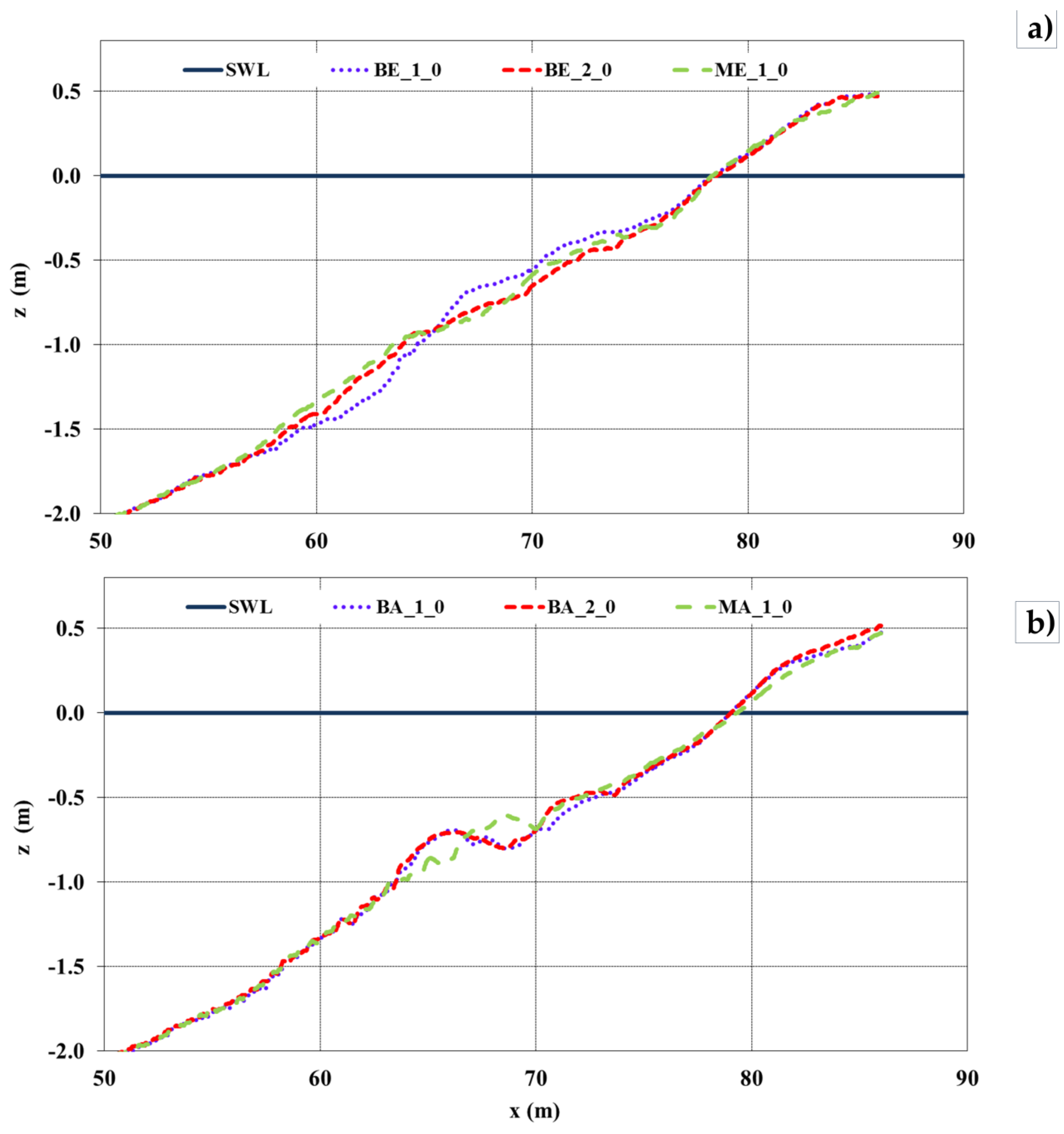
The wave generator system consisted of a wedge type wave paddle, particularly suited for intermediate-depth waves, and a control system implemented by Aalborg University, which accounts for reflection. The absorbing system is particularly functional for higher reflection conditions, i.e., over 30%. Obviously, due to stroke limitations by the paddle, very long waves cannot be effectively adsorbed. The experimental program was divided into two test series, erosive and accretive, respectively. Within each series, a number of different wave cases with identical energy level and energy flux were run, including regular monochromatic and bichromatic waves including bound long waves. Therefore, the cases analyzed here are monochromatics and bichromatics wave conditions, both in erosive and accretive cases. The tests were composed of six steps of 24 min duration. Hence, wave generation was halted and restarted every step duration. On the basis of previous experiments in the CIEM flume and of the typical erosion/accretion threshold criteria based on the relative fall velocity, wave conditions were chosen as likely to be erosive or accretive for the monochromatic conditions. Therefore, the final profiles and net sediment transport are consistent with these initial estimates. Case ME represents the monochromatic control conditions for the erosive test series, with H = 0.37 m, T = 3.7 s at the wave paddle; the profile evolution for the other erosive wave cases are therefore compared to that for case ME. Case MA is the equivalent monochromatic control case for the accretive test series, with H = 0.16 m and T = 4.9 s at the wave paddle.
Four fully modulated bichromatic wave trains were generated, with the intention that each case would have the same theoretical root mean square wave height (and mean energy flux) as its corresponding monochromatic wave. Cases BE_1 and BE_2 generate erosive conditions, and are paired with case ME. Cases BA_1 and BA_2 are paired with case MA and give accretive conditions. The bandwidth of each pair of bichromatic waves is different, and is defined by the frequency difference between the two primary short waves within the group. The specific frequencies were chosen so that the mean energy flux of the pairs of wave trains flux was the same as the corresponding monochromatic waves.
The summary of the experimental program for such tests is reported in
Table 1 and
Table 2. The reader is referred to Vicinanza et al. [
34] for further details.
Prior to running each wave condition, the bathymetry was manually reshaped and then compacted by running 10 min ‘smoothing’ wave condition (random waves with Hs = 0.2 m and Tp = 6 s) in order to obtain almost the same initial profile (
Figure 2). In fact, the following were measured:
The beach evolution along the centerline of the wave flume was measured with a semi-automatic mechanical bed profiler that measures both the sub-aerial and sub-aqueous beach elevation over a range of up to 3 m. The profiler consists of a 0.2 m diameter wheel on a pivoting jib of length 3 m, which is mounted on a carriage that moves at constant velocity above the flume. A software program was used to convert the wheel rotations and the angle of the jib to distance and elevation above a reference level. When the paddle was operating, the profiler’s carriage was in a resting position close to the edge of the beach, and it was used as support for a digital camera.
3. Methods
In the present paper, the hydrodynamic analysis focusses on:
Seiching identification;
Runup estimation.
In particular, two complementary sets of analyses have been carried out for seiching study: a spectral and an eigen analysis. Runup, instead, has been measured by using a digital camera records processing.
The dataset treated in this work concerns the first step for every wave condition. As aforementioned, each test commenced with approximately the same initial profile. Therefore, the influence from morphodynamic feedback during the measurements can be considered unimportant, allowing for determining reliable observations of hydrodynamic response in terms of LFW also in movable bed experiments.
3.1. Seiching Identification
3.1.1. Spectral Analysis
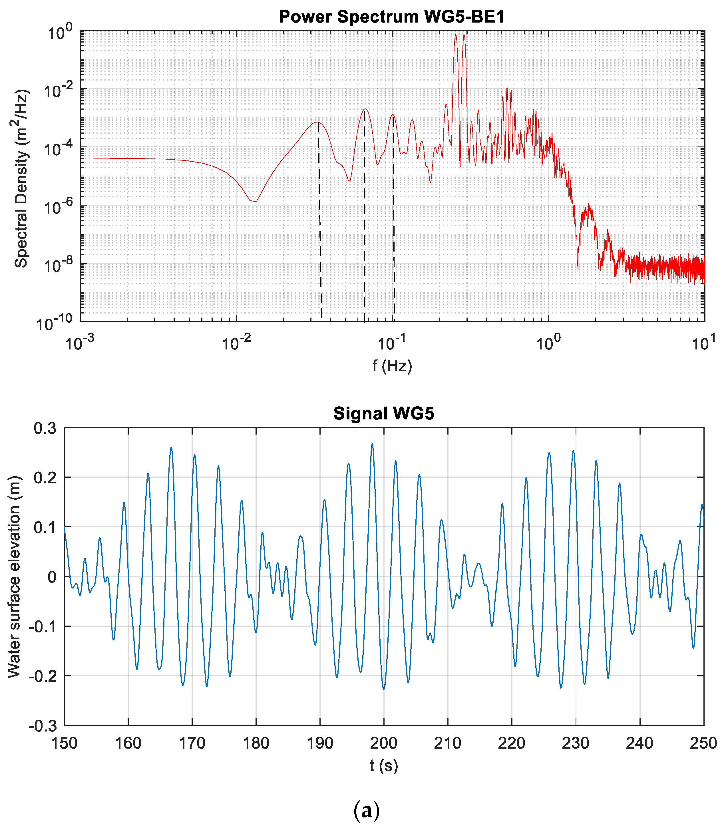
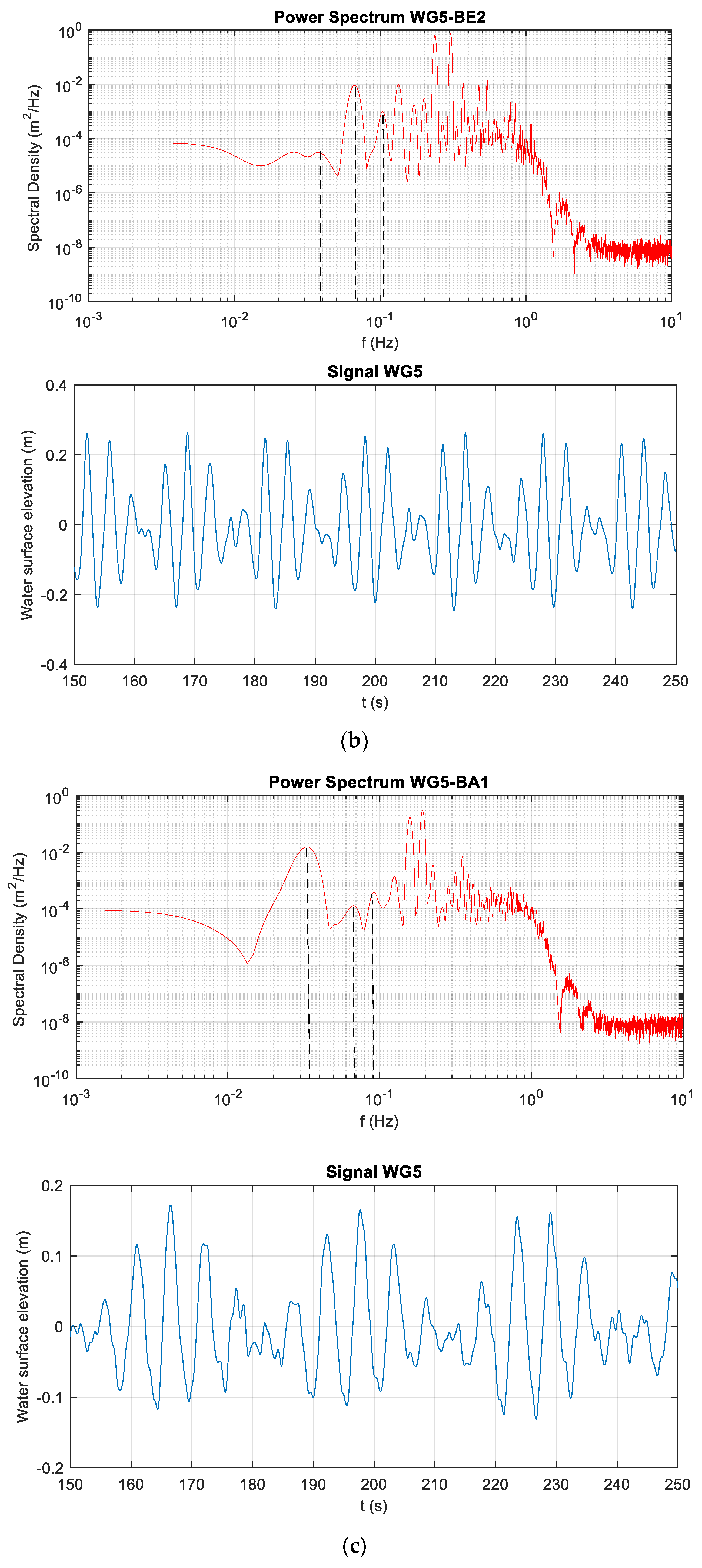
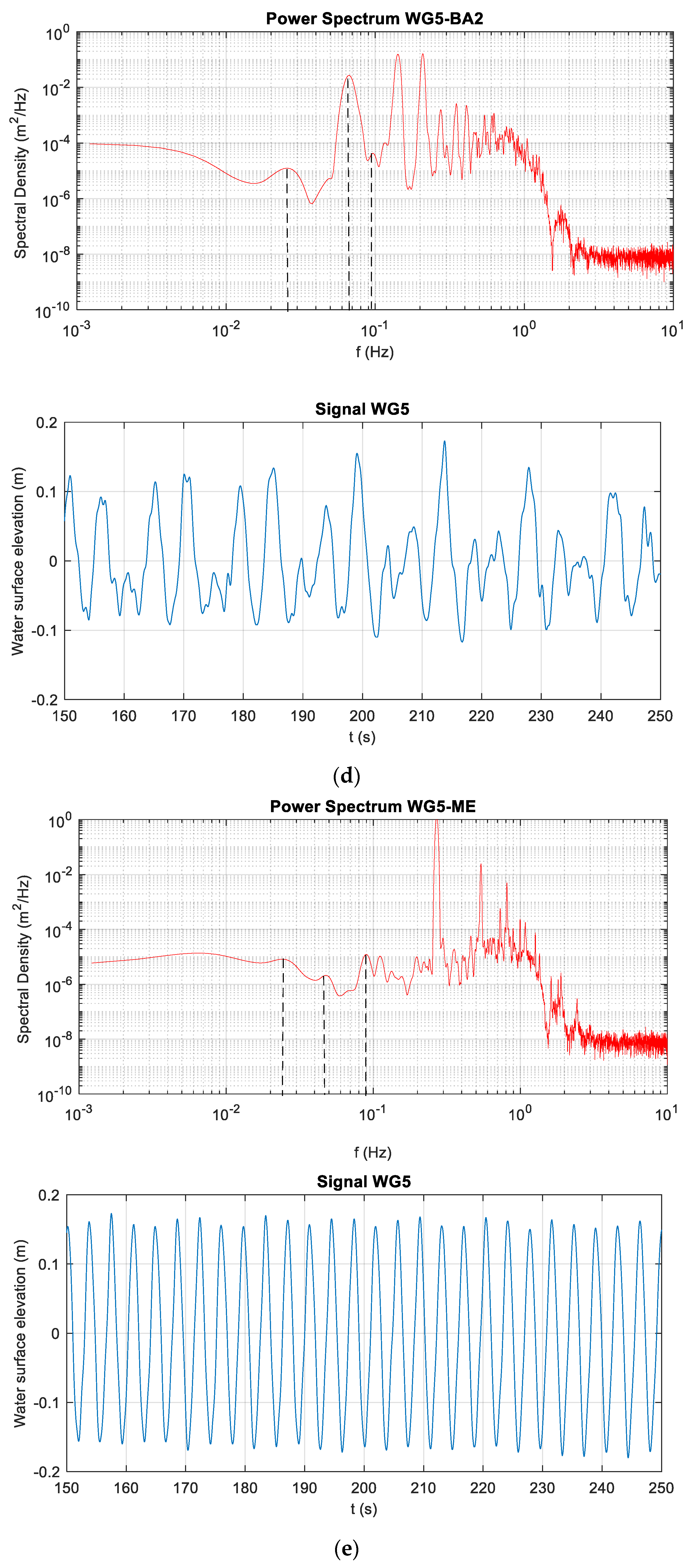
The spectral analysis related to the water surface elevation for all the wave conditions has been carried out in order to analyze the low frequencies.
The power spectral density represents the momentum that corresponds to specific frequencies. A larger amplitude is defined by a higher momentum or spectral density [
41]. Accordingly, in order to perform the spectral analysis for each studied test, a Fast Fourier Transform (FFT) is used through MATLAB™ software (2017b, The MathWorks, Inc., Natick, MA, USA). In particular, a time window equal to the duration of the first step (24 min) has been analyzed without any filtering applied. The analysis has been conducted in order to ensure wave frequencies aligned with FFT bins. First, the spectral peak at low-frequencies range and harmonics are detected. Consequently, the identified peaks are brought into comparison with the wave modes provided by the eigen analysis, as illustrated in the following section.
3.1.2. Eigen Analysis
In order to investigate if the long waves activities are due to or strongly affected by the resonance of specific frequencies (hereinafter “seiche”), an eigen analysis is required. According to Rabinovich [
42], the resonance arises when the dominant frequencies of the external forcing match the eigen frequencies of the wave flume. In particular, in an enclosed basin, seiche is defined as long-period standing oscillation. The resonant (eigen) frequency of the seiche is mainly determined by bottom morphology and overall geometry of the basin. Hence, the set of eigen frequencies, included in the associated modes, is a fundamental property of each basin [
42]. The modes are the number of seiche nodes within the system. The period of a seiche with “
n” nodes is usually described by the so called Merian’s formula [
43]. This approach assumes a rectangular basin with a uniform water depth, for which the period can be computed as follows:
where
Tn is the period of a
nth mode seiche;
L is wavelength of the seiche (basin’s length);
n is the number of nodes/modes of the seiche;
g is gravity’s acceleration equal to 9.81 m/s
2, and
is reference water depth.
Therefore,
Tn can be referred to as the time that the waveform takes to travel a distance of twice the basin length, due to the oscillation from one end of the wave basin to the other and vice-versa. Clearly, seiches with different modes can take place at the same time in a system. However, only one fundamental oscillation is dominant, as previously seen in Wilson [
44].
In the following section, the results of the calculated eigenmodes and eigenvalues derived by applying a numerical approach are presented. The used method, according to Kirby et al. [
45], provides the family of eigenmodes for measured wave flume geometry. The approach takes into account small amplitude seiching in a 1D horizontal canal of depth h(
x). The governing equations are given by the linear long wave equations, as follows:
where η is water surface displacement,
u is horizontal velocity, and
t is the time. The seiching spans the interval 0
≤ x ≤ L. The boundary condition at a wall boundary is taken to be
therefore implying an impermeability condition.
At x = L, the motion remains bounded by the sloping beach.
The elimination of
u is obtained by imposing:
In the case of time-harmonic motion with angular frequency ω, considering λ = ω
2/g as the eigenvalue for the problem, Equation (5) can be rewritten as
Due to the sloping shoreline boundary condition, Equation (6) does not represent a standard Sturm-Liouville problem. The required Liouville transformation leads to the choice of the volume flux,
q = zu, as a dependent variable, giving the following equation:
Equation (7) is finite differenced using centered second-order derivatives. In order to solve the resulting matrix eigenvalue problem, the EIG routine in MATLAB™ software is applied. Equations (8) and (9) provide the corresponding expansion, orthogonality condition, and dispersion relation, respectively:
where
Fn and
Fm represent the family of eigenmodes of order
n and
m, respectively.
In the present study, the four families of eigenmodes, F1, F2, F3 and F4, have been determined by solving numerically Equations (8)–(10).
As demonstrated by Kirby et al. [
45], the method is reliable also in the case of nonlinearity. In fact, the modal amplitude evolution addressed to linear and nonlinear interactions, measured during the large scale experiment at the Hinsdale Wave Research Laboratory [
46], occurred on similar timescales. Such experiments took place in a wave flume with overall dimension and sand characteristics very similar to those of SUSCO experiments. In fact, the wave flume was 104 m long, 3.7 m wide and 4.6 m deep. This helps support the validity of results discussed in the following.
3.2. Runup Estimation
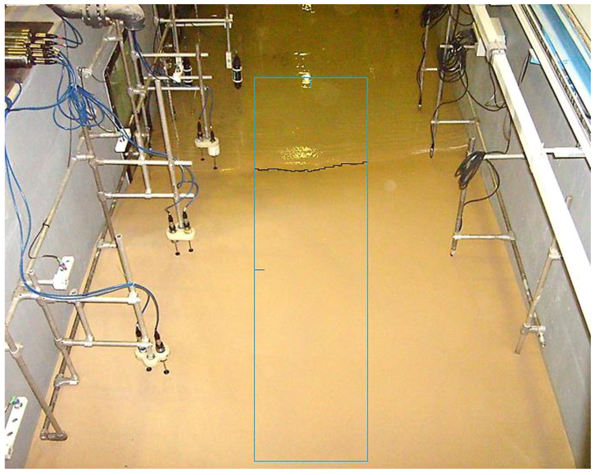
The runup tagging process began from camera calibration phases, by determining the relative position of a minimum of four reference points in the frame. In this study, eight reference points have been considered, in order to define the relative location and orientation of the camera. Target points were the tips of the optical backscatter sensors and the microacoustic wave gauges, the positions of which are known and remain stationary during machining. Once defined in the frame, the coordinates of the frame of reference points, an Image Processing Toolbox™ in MATLAB™ is used to define the relative position of all remaining pixels in the frame (
Figure 3), as described by [
47,
48,
49,
50]. A particular optical filter of the images was applied in order to bring out the visual differences between dry and wet zones. Then, the relative position of runup along the same cross shore section (the centerline of wave flume) was determined as separation between dry and wet zones.
The analyzed videos focused on the first three minutes of each step. Therefore, the computed runup measurements are not significantly affected by morphodynamic changes, since each test starts from the same underlying beach conditions. The good agreement between runup values derived from video analysis and the ones derived on some uprush/backwash cycle extrapolating the measurements from micro-acoustic wave gauges (that only provide the height of the swash lens), provides confidence in the technique.
5. Additional Considerations
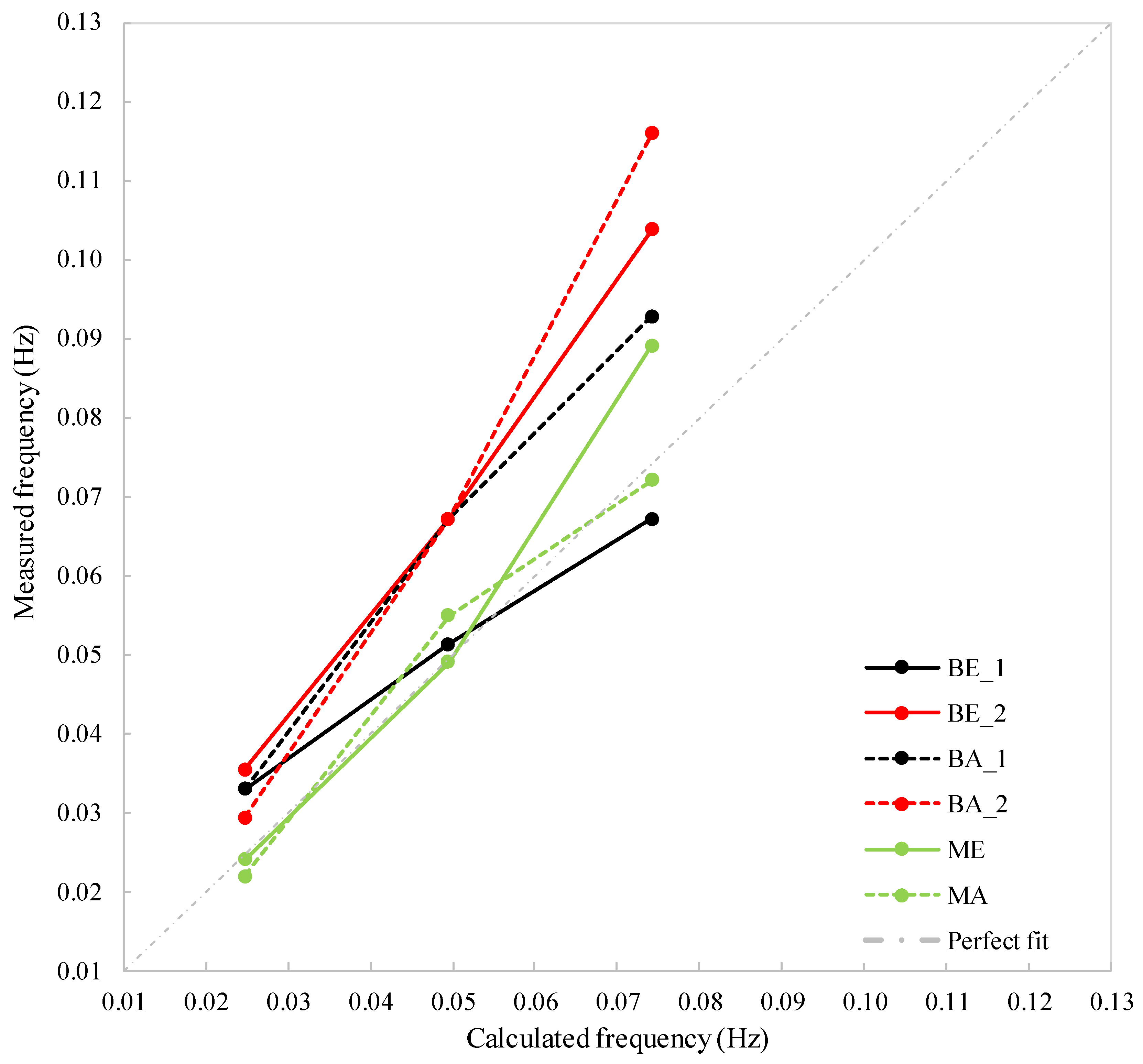
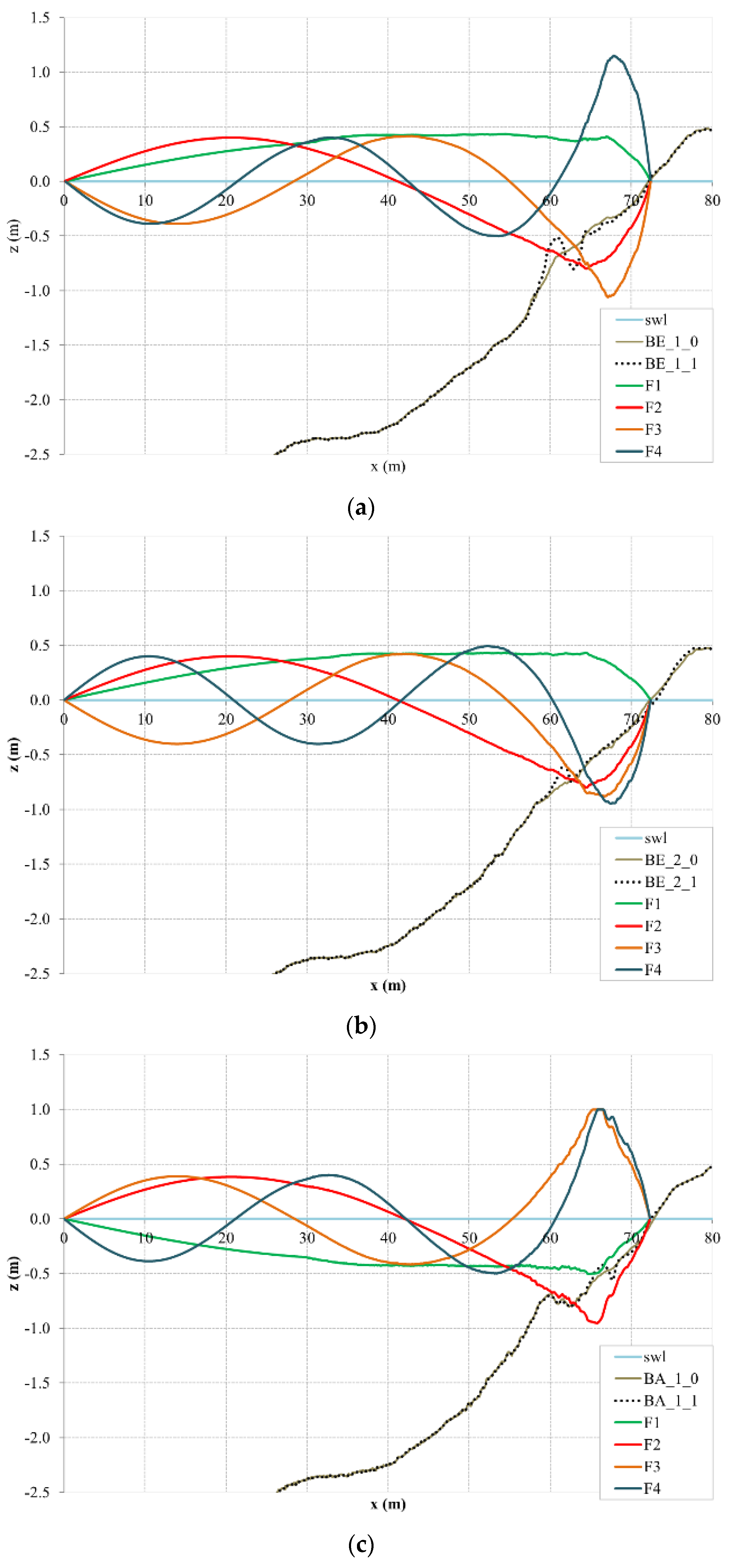
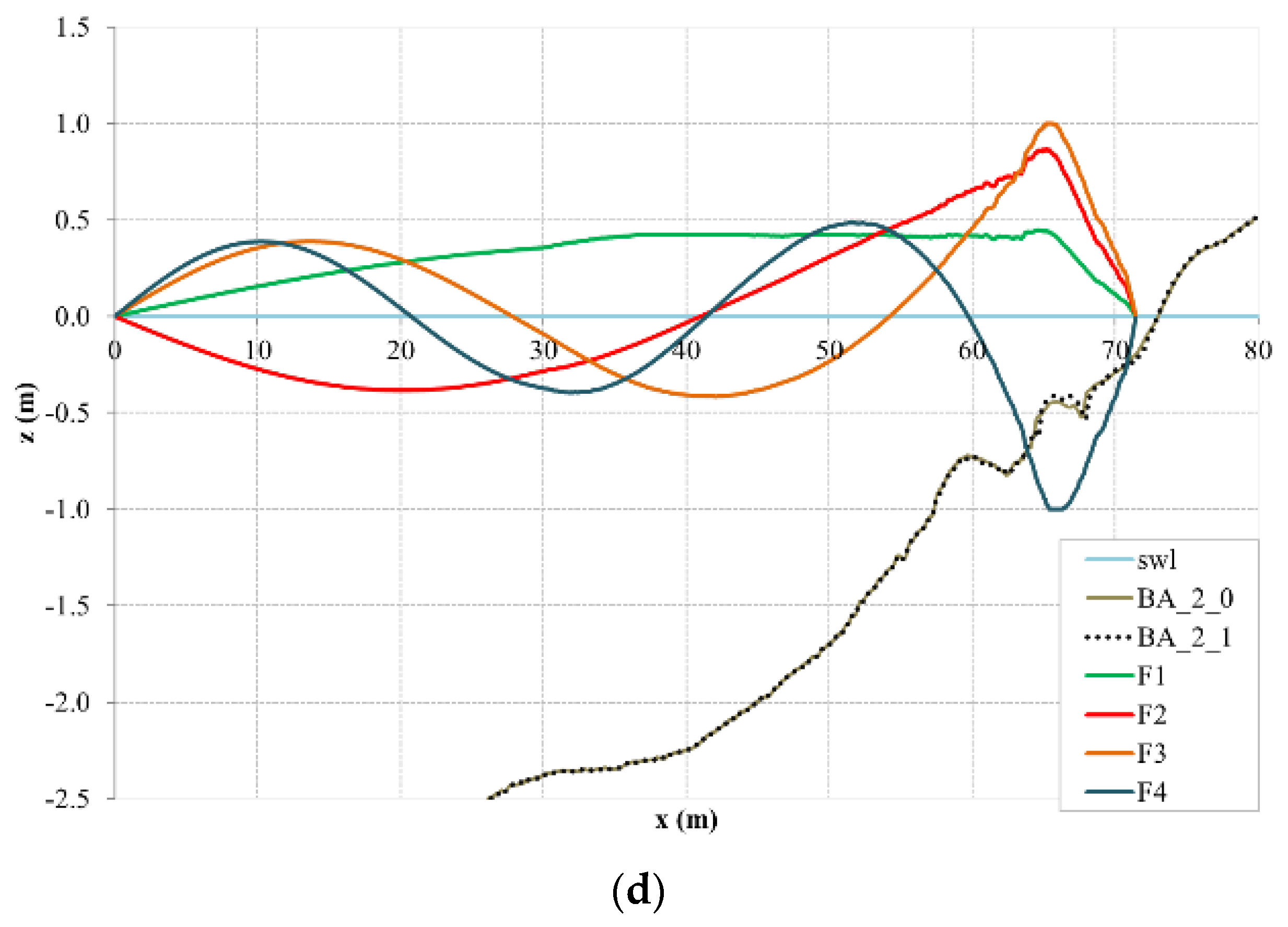
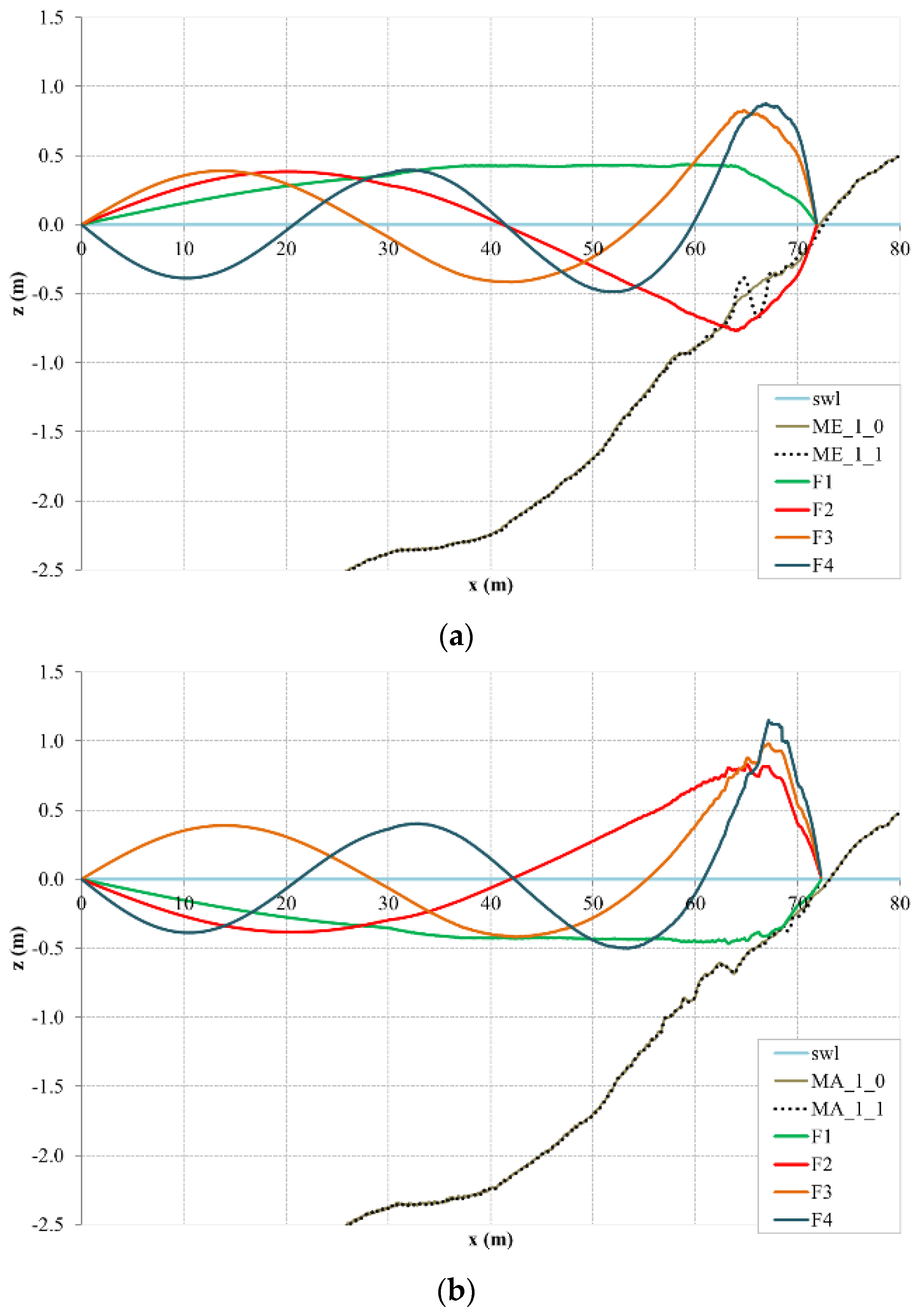
The mode frequencies determined through the eigen analysis—based on water depth z of the wave flume—can represent a powerful tool to highlight the effects of the LFWs and merit further consideration.
In fact, through the computation of the four lowest modes (F
1–F
4) for volume flux in the wave flume (plotted in
Figure 7 and
Figure 8), interesting results can be achieved. A nonlinear pattern of the modes F
1–F
4 is identified near the breaking zone for all studied tests. It is noted that the results corresponding to the bichromatic waves are characterized by nonlinear effects, especially near the breaking point where free long waves are generated [
8,
9]. Therefore, this finding is in accordance with Longuet-Higgins and Stewart [
53,
54] since the bichromatic wave groups force an associated bound long wave at the group frequency.
An opposite behavior of volume flux eigenmodes is shown for the fourth mode F
4 of the BE_1 and BE_2 cases (
Figure 7a,b). Furthermore, for the first and second mode, a dependency of the different bandwidths for bichromatic waves in accretive conditions is observed (
Figure 7c,d).
The eigenmodes for volume flux, q, related to the profile measured in the monochromatic tests show a different variation probably due to the nonlinearity effects for the first and second modes in both erosive and accretive conditions.
The harmonic disturbance for bichromatic waves with narrower and larger bandwidth could lead to erosion phenomena where the formation of well visible bars is seen. The resulting profiles and net sediment transport were consistent with these initial estimates [
34].
Moreover, it is worth noting that the local effect on a beach profile of bichromatic or monochromatic waves can be significantly different due to the interaction of the LFWs that affects the spectra. Considering the typical pattern of modes F
1–F
4 (according to [
45,
52]), some differences can be observed in
Figure 8. In fact, it is identified:
an accretive pattern in the case of bichromatic waves BE_1 for the fourth mode F4;
an erosive behavior for the second mode in BA_1;
an erosive structure for the first and fourth mode in case BA_2;
an accretive pattern for the F3 and F4 in ME;
a completely erosive pattern for MA case.
Influence on Swash Zone Sediment Transport
In the swash zone (SZ), the dissipation of short-wave (wind and swell) energy occurs, while the LFW energy is generally reflected back seaward. Moreover, intense short-short and short-long wave interactions at the surf-swash boundary can influence the generation and reflection of further LFWs [
55,
56]. Superficial SZ hydrodynamics, subsurface SZ hydrodynamics, sediment dynamics and co-related beachface morphodynamics are strongly determined by the swash motion’s frequency in non-tidal regimes [
57,
58,
59,
60,
61]. Therefore, for low frequency motions and sediment transport, important feedback can be found, according to Russell [
62] and Smith and Mocke [
63]. LFWs, in particular, lead to mobility of the sediment into suspension by the short waves.
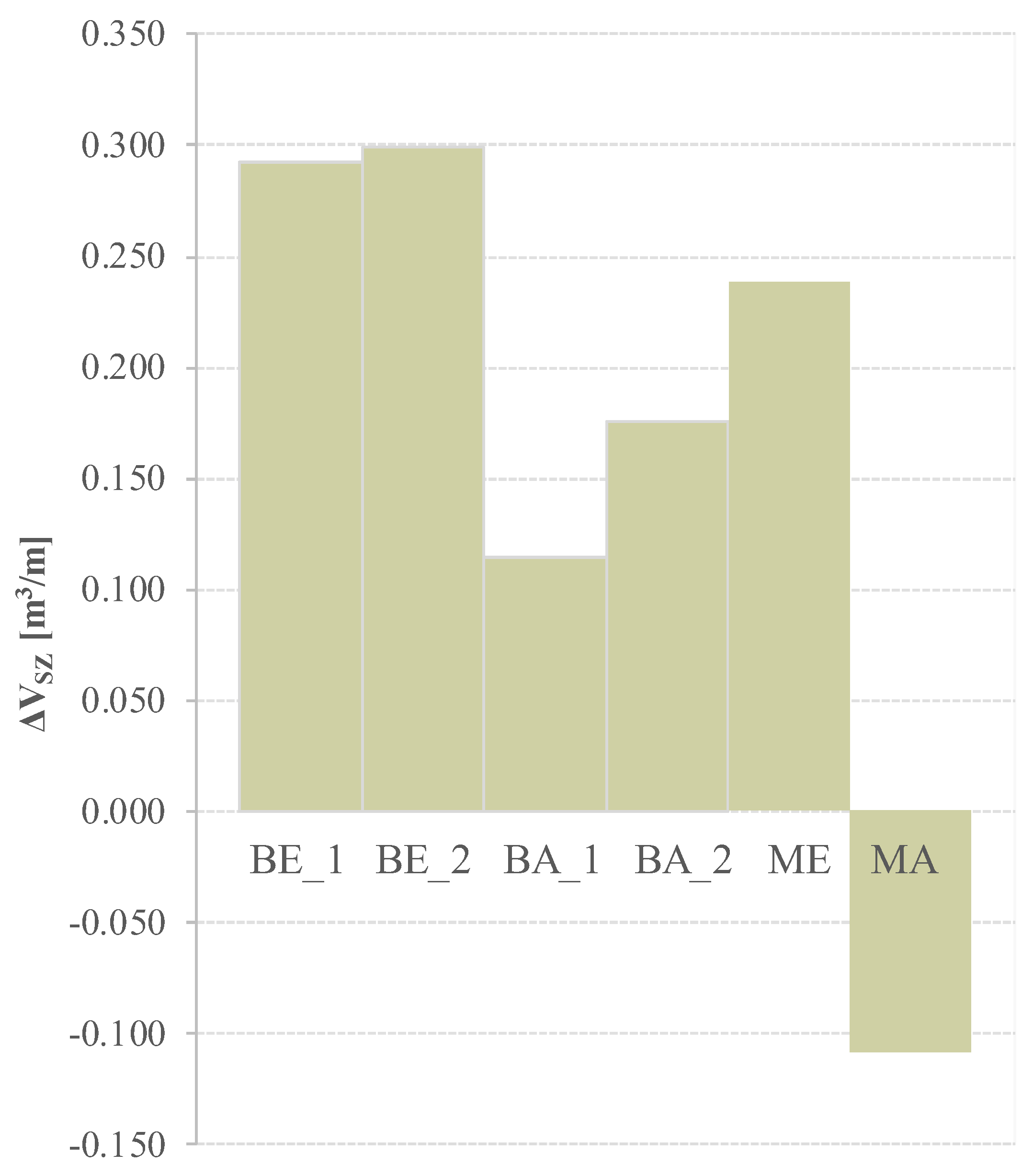
Based on this reasoning,
Figure 9 shows the net sediment volume variation in the SZ, and ΔV
SZ, approximated as the emerged beach, between the start and end of the test is provided. Such a variation is determined by applying changes in bed elevation between profiles above the SWL.
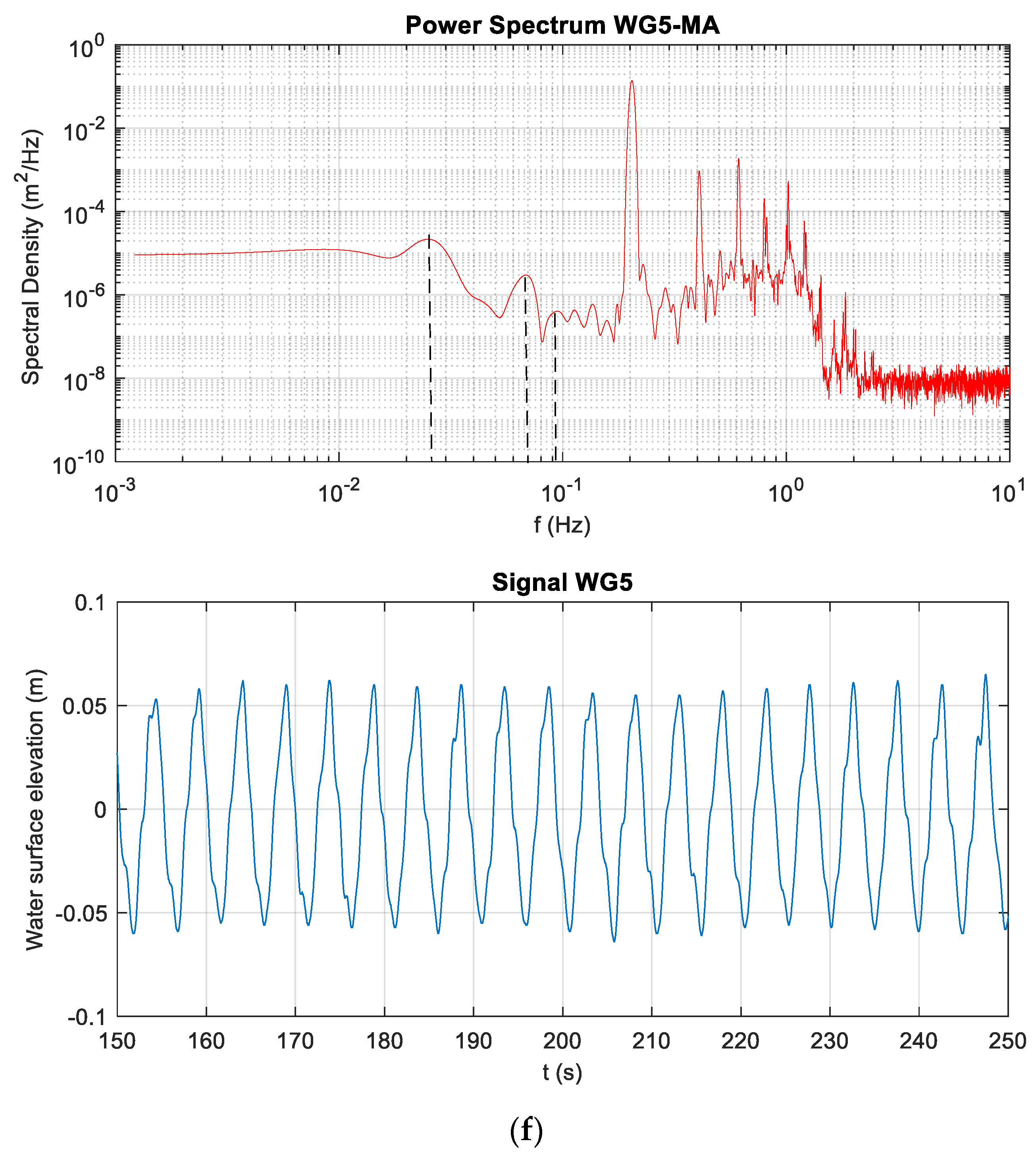
It is observed that all wave conditions related to the first step of experiments lead to a landward net sediment transport, except for case MA. In particular, for bichromatic waves with narrower bandwidth, the power spectral density associated with the first harmonic has been found larger than the power level of the second mode, increasing the disturbance effect of the 1st harmonic itself. On the contrary, for the bichromatic waves with larger bandwidth, the power spectral density associated with the second harmonic is larger than the energy of the first mode, increasing the disturbance effect of the 2nd harmonic. Therefore, the different bandwidths of the bichromatic waves are found to be influenced by the low frequency motions.
Furthermore, the net sand volume variation in the emerged swash zone is greater in the erosive condition than the accretive condition for bichromatic waves. Consequently, a morphological effect is observed in which the different bandwidths could promote the presence of the low-frequency motions responsible for nonlinear interactions.
It is also noted that the net sand volume variation in the emerged swash zone is higher in the erosive cases than those determined in the accretive cases, showing positive values. This behavior is in line with the typical erosion pattern along the profile of the bichromatic and monochromatic waves under erosive conditions. In particular, this effect is produced by the initial profiles during the experimental campaign with the same initial conditions. Therefore, the beach variations associated with the erosive cases arise when the equilibrium profile is reached, and the mean beachface slope changes. Hence, at the beginning of the tests, erosion of sediment provides some local deposition with positive slope change. What is also important is the erosive pattern under accretive monochromatic conditions. Here, the effect of resonance could be more evident; therefore accretive wave conditions could provide sweetening of the swash zone slope, by behaving more in a slightly erosive pattern.
6. Conclusions
A data set from controlled large-scale experiments at UPC were specifically used to identify seiching from various wave regimes and their effects on spectral components. In particular, monochromatic and bichromatic wave groups with different bandwidths were analysed.
In order to discriminate low frequency components, an eigenvalue decomposition was carried out. Comparing measured and calculated eigenvalues, an appreciable correspondence for the first harmonic has been found for all the bichromatics tests. Consequently, a wave flume-generated signature of the first harmonic can be identified. Moreover, for the monochromatic and the erosive bichromatic wave conditions with narrower bandwidth, a good correlation for other harmonics was also detected.
Results suggested that the wider bandwidth had the higher ratios between the spectral density of the second and first harmonic and the lower ratios between spectral density of the 2nd/1st and 3rd/2nd. Specifically, in enlarging the bandwidth:
the highest power spectral density peak downshifted toward the second harmonic;
enlargement of the swash zone was promoted and the runup values (in comparable morphodynamic initial condition) increased significantly;
moving from the same initial profile, the sediment transport rate and related swash zone morphological changes became more important.
The effect of resonance was highlighted by a volume flux eigenmode analysis. For all the studied tests, a pattern of energy exchange between modes has been determined. In particular, the results related to the completely erosive pattern of F1–F4 modes in the MA case and the accretive pattern for F3–F4 in the ME case and the fourth mode in BE_1 case were consistent with the computed volume variation in the emerged swash zone. Hence, it appeared that the seiching effect could influence the interaction between successive swash events (swash-swash interaction) and the interaction between standing waves and incident bores on runup. Such interaction may be constructive or destructive in hydro-morphodynamics terms.
It is appropriate to point out that in the swash zone the magnitude of net sediment volume suggests that low frequency oscillations could have a significant influence only on generation/development of secondary bedforms.
Further work is required to better understand quantitative implications of seiching in laboratory experiments for sandy slope profiles. Particularly, in order to investigate the seiching response when an equilibrium profile is achieved, including the morphodynamic feedback is important and additional analyses should be attempted on the last steps of each test of the UPC dataset.


