Article

Influence of Propulsion Type on the Stratified Near Wake of an Axisymmetric Self-Propelled Body

by
Matthew C. Jones
1,* and
Eric G. Paterson
2
1
Department of Aerospace and Ocean Engineering, Virginia Polytechnic Institute and State University, Blacksburg, VA, 24061 USA
2
Department Head and Rolls-Royce Commonwealth Professor of Marine Propulsion, Department of Aerospace and Ocean Engineering, Virginia Polytechnic Institute and State University, Blacksburg, VA 24061, USA
*
Author to whom correspondence should be addressed.
J. Mar. Sci. Eng. 2018, 6(2), 46; https://doi.org/10.3390/jmse6020046
Submission received: 1 March 2018 / Revised: 30 March 2018 / Accepted: 23 April 2018 / Published: 1 May 2018
(This article belongs to the Special Issue Marine Propulsors)

Abstract

:
To better understand the influence of swirl on the thermally-stratified near wake of a self-propelled axisymmetric vehicle, three propulsor schemes were considered: a single propeller, contra-rotating propellers (CRP), and a zero-swirl, uniform-velocity jet. The propellers were modeled using an Actuator-Line model in an unsteady Reynolds-Averaged Navier–Stokes simulation, where the Reynolds number is R e L = 3.1 × 10 8 using the freestream velocity and body length. The authors previously showed good comparison to experimental data with this approach. Visualization of vortical structures shows the helical paths of blade-tip vortices from the single propeller as well as the complicated vortical interaction between contra-rotating blades. Comparison of instantaneous and time-averaged fields shows that temporally stationary fields emerge by half of a body length downstream. Circumferentially-averaged axial velocity profiles show similarities between the single propeller and CRP in contrast to the jet configuration. Swirl velocity of the CRP, however, was attenuated in comparison to that of the single propeller case. Mixed-patch contour maps illustrate the unique temperature distribution of each configuration as a consequence of their respective swirl profiles. Finally, kinetic and potential energy is integrated along downstream axial planes to reveal key differences between the configurations. The CRP configuration creates less potential energy by reducing swirl that would otherwise persist in the near wake of a single-propeller wake.

1. Introduction

Experiments show that propeller-driven wakes evolve from a complicated near wake with discernible propeller-blade features, to a far wake, in which these features have mixed together to form a nearly-axisymmetric field [1,2]. Sirviente and Patel [3] show that the near-wake region transitions to the far wake in roughly twelve initial wake diameters, but the development of the far wake can be delayed by appendages on the body [4]. This transition is influenced by the Reynolds number, body geometry, and operation of the propulsor [5], which itself has a large impact on the ingested stern boundary layer and downstream turbulence [6,7]. The swirling propeller induces helical vortices that are shed from the roots and tips of the individual blades. In the near wake, these vortices break down, which is a topic of extensive study [8]. Although experiments show the contribution of swirl [9], its role in the evolution from near to far wake is not well-characterized.
In a stratified wake, a mixed patch is formed by swirl from the propeller, turbulent mixing, and potential effects from the upstream body [10]. This mixed patch can further modify the far wake in the event of a mixed-patch collapse when buoyancy forces are large [11,12,13,14]. Numerous experiments have explored the interaction between stratification and wake evolution with close observation to the generation of internal gravity waves and coherent structures [15,16]. Direct Numerical Simulation (DNS) provides further insight into the physics of the flow, particularly with its turbulence properties [17,18]. Background turbulence increases the turbulent kinetic energy and energy transfer in the wake, which in turn lowers the mean velocity and increases horizontal spreading [19]. Excess momentum leads to changes in increased turbulent kinetic energy and qualitative changes in the wake dynamics, particularly in downstream vortical structures [20]. High levels of stratification in the wake create a non-equilibrium region in which the mean velocity decay is reduced [21,22]. By reducing the level of potential energy in the near wake thermal-haline distribution, the effects of buoyancy in the far wake can be reduced.
Originally studied as a disc-with-center-jet [23] and later with self-propelled axisymmetric bodies [24,25], the net-zero-momentum wake functions as a theoretical model of a self-propelled marine vehicle. Beyond experiment, the study of self-propelled wakes includes several numerical methods. Ordered by increasing fidelity and computational expense, these methods include [26]: panel/lattice methods, actuator models, and fully resolved rotating geometry. Generalized actuator models include the Actuator Disk (AD), Actuator Line (AL), and Actuator Surface (AS) models. Each of these models imposes a body force over a volume in a Computational Fluid Dynamics (CFD) simulation to simulate the effects of a propeller on the surrounding fluid. Although a fully resolved propeller may offer more fidelity, its computational requirements are often large, so an actuator model provides a cost-effective alternative [27].
In a self-propelled near wake, the mixed-patch structure and overall potential energy depend largely on the propulsor. A single propeller will mix fluid unopposed within the swirling region of the wake. Contra-rotating propellers of equivalent thrust will modify the initial swirl profile thereby changing the shape of the downstream mixed patch and reducing its potential energy. Contra-rotating propeller blades add additional complexity to the interaction between root and tip vortices and reduce the swirling kinetic energy of the wake. These influences on the near wake may be compared to the simplified case of a zero-swirl, jet-propelled configuration with uniform-velocity, which results in the smallest generation of the potential energy in the wake.
The present study is an extension of Jones and Paterson [28]. The unsteady Reynolds-Averaged Navier–Stokes (URANS) equations are solved to examine the near-wake evolution of the stratified, turbulent, net-zero-momentum propeller wake of the axisymmetric Iowa Body using three different propulsion schemes: single propeller, dual contra-rotating propellers (CRP), and a zero-swirl, uniform-velocity jet. The propellers are simulated using the AL model. The Iowa Body hull geometry is chosen for comparison to the non-stratified experiment by Hyun and Patel [2], which is the only known experiment to have phase-averaged propeller data for a self-propelled axisymmetric body. The authors have previously shown good agreement to this experiment for towed and self-propelled configurations [27]. Flow visualization reveals the interaction between propeller-root and tip vortices and the additional complexity introduced by CRP. Comparison between instantaneous and time-averaged cross-plane profiles demonstrates the transition from near- to far-wake regions. Circumferentially-averaged profiles of velocity reveal the evolution of momentum, with observations drawn in comparison to the theoretical disc-with-center-jet that is often used in far-wake simulations [11]. Mixed-patch velocity and temperature-deviation cross-plane profiles show the structure of kinetic and potential energy in the developed wake. Finally, the relative growth, decay, or persistence of integrated kinetic and potential energy of each propulsion scheme is considered. Compared to the single-propeller configuration, the CRP configuration is more effective at reducing potential and swirling kinetic energy in the wake, with potential energy reductions similar to that of the zero-swirl jet.

2. Approach

2.1. Governing Equations

This fluid-flow problem is defined by the unsteady Reynolds-averaged Navier–Stokes (RANS) equations in Boussinesq form with an additional body force term f p to account for the propeller model.
U j x j = 0
U i t + ( U i U j ) x j = 1 ρ 0 p ^ x i + ν 2 U i x j x j + x j u i u j ¯ + Δ ρ ρ 0 g j δ i j + 1 ρ 0 f p
The equations are written in terms of the non-inertial velocity U i . In the equations, t is time, ν is the kinematic viscosity, and ρ is density. The density is expressed as ρ = ρ 0 + Δ ρ , where ρ 0 is a reference value and Δ ρ is the deviation from that value. The gravitational vector g j points downward in the negative z direction, where z is the upward-positive, vertical position. This formulation includes the piezometric pressure, p ^ = p ρ 0 g z where g is the magnitude of the gravitational vector.
The governing equations are solved using a custom solver written with the CFD framework OpenFOAM. This custom solver takes into account salinity and temperature transport and the corresponding turbulent fluctuations. The transport of temperature T and salinity S in the stratified environment are determined through the following equations with the diffusion coefficients κ T and κ S .
T t + ( U j T ) x j = κ T 2 T x j x j + x j u j t ¯
S t + ( U j S ) x j = κ S 2 S x j x j + x j u j s ¯
The Reynolds stresses u i u j ¯ and turbulent fluxes u j t ¯ and u j s ¯ are determined using a linear eddy-viscosity closure model.
u i u j ¯ = 2 ν t S i j 2 3 k δ i j
u j t ¯ = ν t σ T T x j
u j s ¯ = ν t σ S S x j
In these equations, ν t is the eddy viscosity, S i j is the mean rate of strain, and k is the turbulent kinetic energy. For this study, the k ω SST turbulence model is chosen to compute ν t due to its ease of implementation and relative advantage in computing the attached flow over a body [29]. Production terms in the k ω equations are modified to include buoyancy effects, but in the near wake they are small in comparison to the production due to shear. Wall functions are used in the computation of k and specific turbulence dissipation ω at wall boundaries to relax mesh requirements near the hull in the high Reynolds-number flow.
Density is computed by solving the UNESCO seawater equation of state [30]. For the given problem, it is appropriate to approximate the secant bulk modulus as constant at sea-level conditions, even though it is a function of salinity, temperature, and pressure. Thus, the secant bulk modulus is K ( S , T , p ) = K ( 0 , 20 , p a t m ) where p a t m is atmospheric pressure. Additionally, substituting the hydrostatic pressure for the total pressure, the equation of state becomes,
ρ ( S , T , p ) = ρ ( S , T , 0 ) 1 p / K ( S , T , p )
ρ ( S , T , 0 ) = a 0 + a 1 T + a 2 T 2 + a 3 T 3 + a 4 T 4 + a 5 T 5 + b 0 + b 1 T + b 2 T 2 + b 3 T 3 + b 4 T 4 S + c 0 + c 1 T + c 2 T 2 S 3 / 2 + d 0 S 2
where a n , b n , c n and d 0 terms are empirical coefficients given in Table 1. Because the environment in the present study is isohaline, only changes in temperature from the thermally-stratified background affect changes in density.

2.2. Kinetic and Potential Energy

The evolution and transfer of energy in the wake is examined in the form of kinetic and potential energy defined as,
k e = 1 2 ρ U 2 , p e = 1 2 g ρ 0 / z ( ρ ρ 0 ) 2
K E = A k e d A , P E = A p e d A ,
The per-unit-volume energy k e , and p e may be integrated over an axial slice of area A in the wake to find energy per-unit-length, K E and P E , as functions of downstream distance. Kinetic energy is computed for the magnitude of velocity and also individually for each component of velocity in cylindrical coordinates. The potential energy per-unit-volume pe follows the formulation of Holliday and McIntyre [31].

2.3. Actuator-Line Model

The unsteady propeller for each non-BOR hull form is simulated using an AL model from the Simulator fOr Wind Farm Applications (SOWFA) library [32]. The AL model projects a distributed line of force f p in the place of each propeller blade,
f p ( r ) = F p ε 3 π 3 / 2 exp r ε 2
where F p is the actuator element force composed of contributions from lift F L and drag F D . The distance between CFD cell center and actuator point is r, and ε controls the Gaussian width. This function decays to 1% of its maximum value when ε = 2.15 r . If ε is too small, numerical oscillations arise, and if ε is too large, the applied body forces will be smoothed considerably. Troldborg [33] recommends ε 2 Δ x where Δ x is the grid spacing at the actuator position. Martınez et al. [34] developed best practices for AL modeling and suggested ε > 2 Δ x . For the present study, ε 4 Δ x was selected because it eliminated the numerical instabilities that arose when ε 2 Δ x was assigned. The Cartesian-mesh region of the propeller was refined to a resolution such that, Δ x / Δ b = 0.74 , where Δ b is the width of each hydrofoil section. Martınez et al. [34] suggests a value smaller than 0.75. Lift and drag at each section are computed from a lookup table of lift and drag coefficients C and C d as functions of α ,
F L = 1 2 C ( α ) ρ U r e l 2 c w , F D = 1 2 C d ( α ) ρ U r e l 2 c w
where ρ is the density, U r e l is the local flow speed, c is the chord and w is the width of the actuator section. The relationship between C and C d with α must be predetermined from experiment, simulation, or theory for each hydrofoil section. 
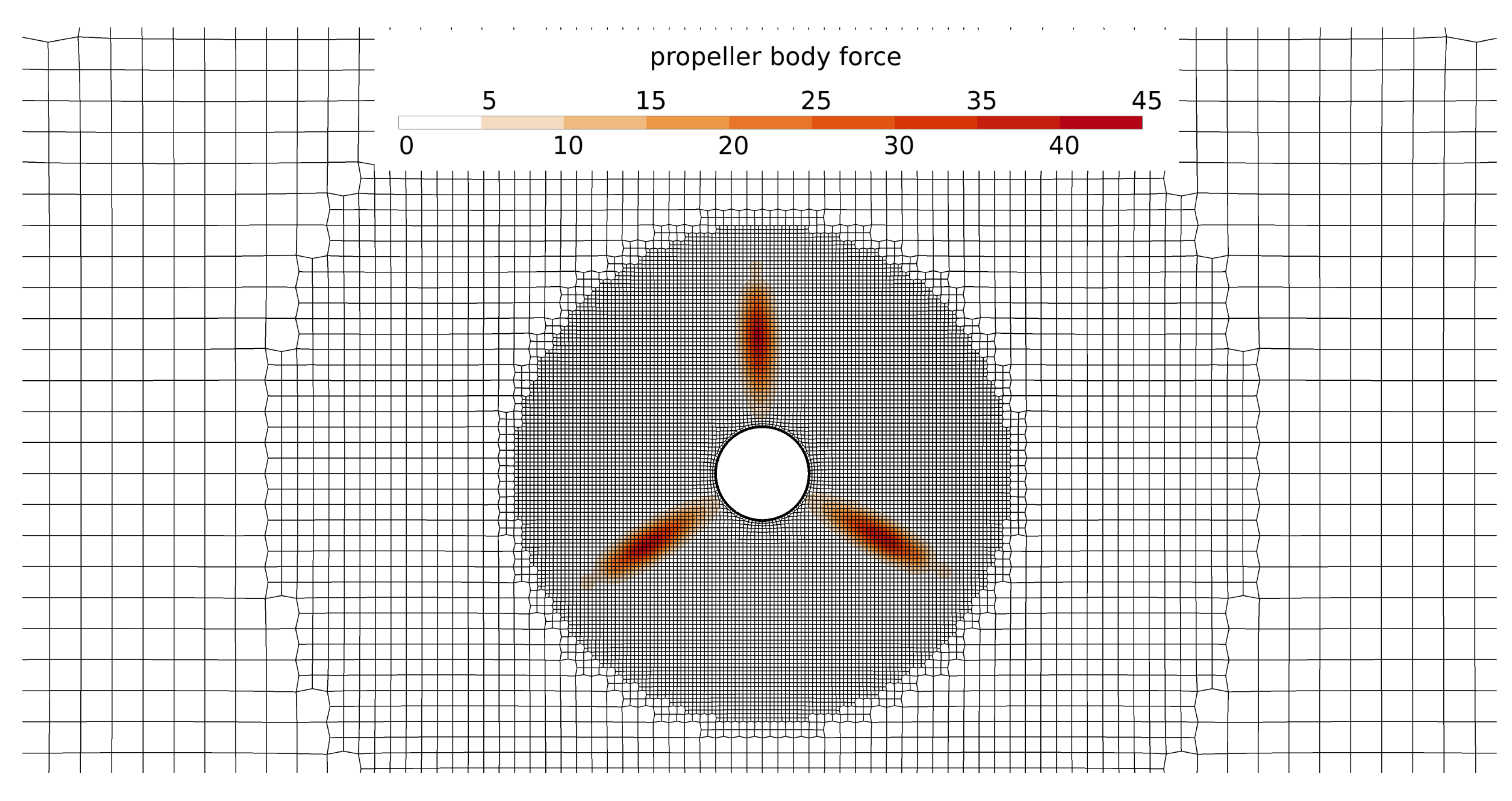
Figure 1 shows the magnitude of the projected propeller body force | f p | / ( ρ 0 R p rps 2 ) on the AL propeller plane of the single-propeller case, where R p is the propeller radius and rps is the propeller rotations per second.

2.4. Iowa Body

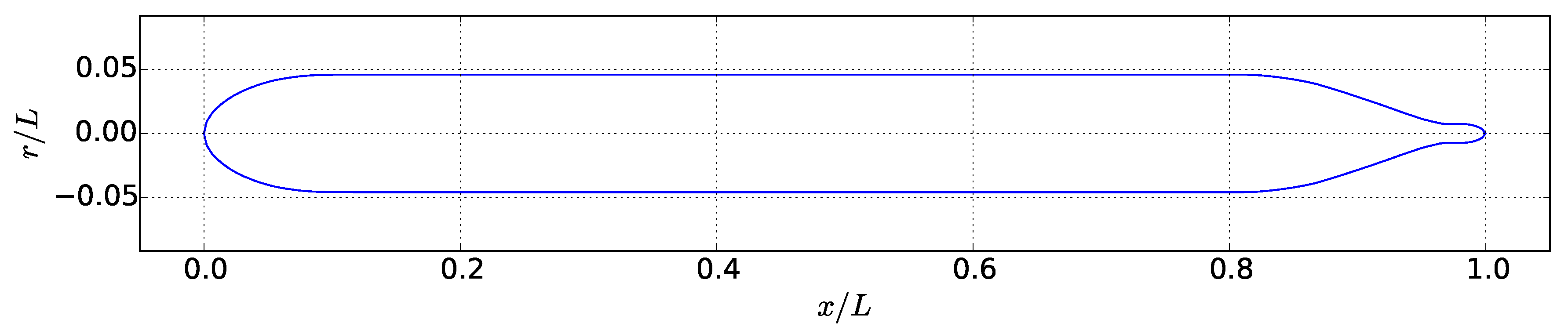
The axisymmetric Iowa Body, described in the experiment by Hyun and Patel [2], is shown in Figure 2 for the standard, single-propeller case. This geometry is representative of a typical marine vehicle without appendages. Features of this geometry are listed in Table 2 where L is the body length, D is the body diameter, D p is the propeller diameter, and D h is the hub diameter.
Minor modifications are made to the Iowa Body hull for the CRP and jet configurations. For the CRP configuration, the hub is extended by the length of the rotating portion so that a second propeller may be placed directly downstream of the first. For the jet configuration, the hub is truncated at the propeller plane to function as an exhaust port. In effect, the zero-swirl, uniform-velocity jet exhausts with an initial diameter of D h .

2.5. Iowa Body Propeller

The Iowa Body propeller is defined by 36 discrete sections to account for variations in radial propeller-blade geometry. Sectional lift C is computed using the analytic expression of Brockett [35] for the NACA 66-Modified foil,
C = 2 π ( 1 0.83 τ ) ( α + 2.05 f )
where α is the local flow angle of attack, τ is the maximum thickness ratio, and f is the maximum camber ratio. Sectional drag C d is imposed by combining viscous and induced drag at each section,
C d = C d 0 + C 2 π e AR
where C d 0 is the viscous drag, e is the efficiency factor, and AR is the aspect ratio.
For the present unsteady simulations, α at each section of the propeller blades remains below 3 at every instant in time. Because α remains small, these analytic expressions do not require additional conditions for stall. Pitch, chord, thickness, and camber distributions for the Iowa Body propeller blade are tabulated in Hyun [1]. The Iowa Body propeller has zero rake and zero skew.

2.6. Computational Mesh

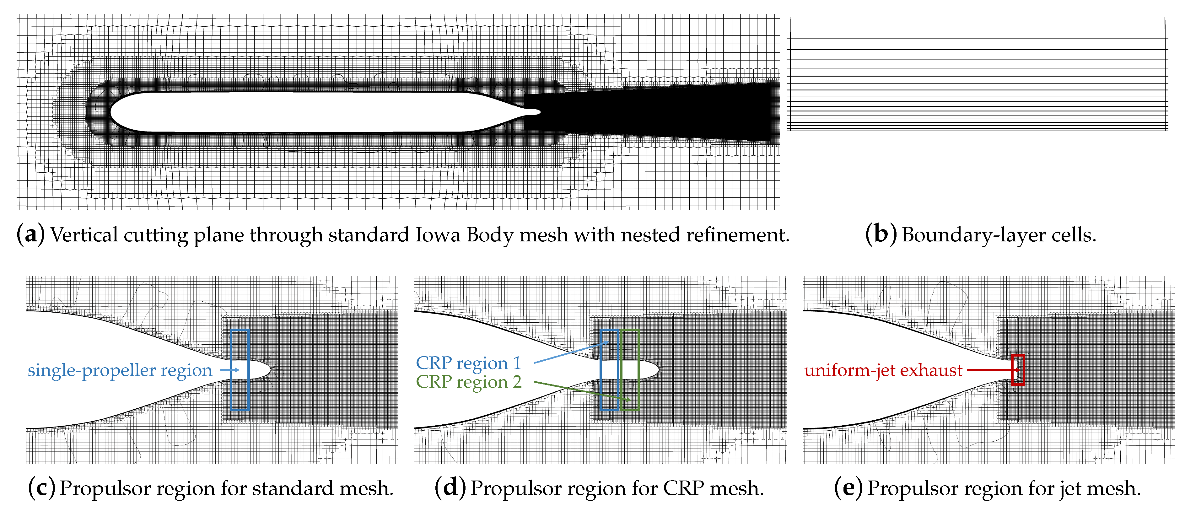
The three computational meshes were generated using the software cfMesh [36]. Cells are focused near the body, the propulsor region, and in the wake. The hull is located at a depth of one body length. The inlet, outlet, and far-field boundaries are located two body lengths away from the hull. Comparison to simulations from spatially-larger meshes showed that the boundaries of the computational domain did not affect the solution. Mesh design and quality features are listed in Table 3. Because wall functions are used in the computation of turbulence variables, the dimensionless wall distance requirement of y + < 100 can capture the boundary layer effects and the viscous drag of the hull even for boundary cells where y + 100 . A grid-refinement study of the propeller- and wake-region cells showed that 100 cells/ D p adequately resolved the AL model and downstream wake cross-plane profiles. These meshes are also visualized in Figure 3. Cutting planes reveal the distribution of cells surrounding the hull and in the wake region. Views of the propulsor region show how the mesh is modified for each configuration. A single AL-modeled propeller is implemented within the highlighted region for the single-propeller case. For the CRP configuration, the hub is extended with one AL-modeled propeller placed behind the first. There is no AL model for the jet configuration since there is no propeller. Instead, fluid is exhausted from the truncated hub.

2.7. Numerical Methods

The Navier–Stokes unsteady mass and momentum equations are solved using the Pressure-Implicit with Splitting of Operators (PISO) method [37]. This segregated approach decouples operations on pressure and velocity variables. At each time step, the following procedure is followed in the customized OpenFOAM solver. First, the momentum equations are solved to provide velocity by using pressure from the previous time step. Next, the pressure-Poisson equation is solved iteratively with corrections to velocity to conserve mass. Three inner iterations are are used in the present study, each with an additional mesh non-orthogonality correction step. After completion of these inner iterations, turbulence quantities are solved for, followed by salinity and temperature. The time step is then advanced.
Implicit, second-order, backward differencing is used in temporal discretization, while the cell-centered finite volume method is used in spatial discretization. A second-order, linear-upwind scheme is applied to the advective term of the momentum equations. A first-order, upwind scheme is applied to turbulence quantities, and a second-order, linear scheme is applied to all other divergence terms. Laplacian terms are discretized using a second-order, linear scheme that is partially-limited to correct for mesh non-orthogonality.
Two iterative methods are employed to solve the resulting systems of algebraic equations. The pressure equation is solved using the Preconditioned Conjugate Gradient (PCG) method with a residual tolerance of 10 6 . The momentum, scalar transport, and turbulence equations are solved using the Pre-Conditioned Bi-Conjugate Gradient (PBiCG) scheme with a residual tolerance of 10 8 .

2.8. Initial and Boundary Conditions

Several boundary conditions are employed. Velocity at the inlet is set to the freestream velocity U 0 through a Dirichlet boundary condition. The no-slip condition is set on the hull boundary, and the slip condition is set in the far field. Zero-gradient conditions are specified for velocity and pressure in the outlet. Background turbulence values of k and ω are computed assuming a turbulence intensity of 1% and eddy viscosity ratio ν t / ν of 100. Turbulence variables on the hull boundary are computed with wall functions. Other variables satisfy the zero-gradient Neumann boundary condition.
Initial conditions for pressure and velocity are computed by solving the potential flow equations. The PISO algorithm is then used in the transient simulation. Distributed body forces from the propeller-blades rotate at each time step at the propeller’s rotation rate. The simulation is then run until initial-transient flow features advect far downstream and a periodic wake flow field is found.

2.9. Flow Field Analysis

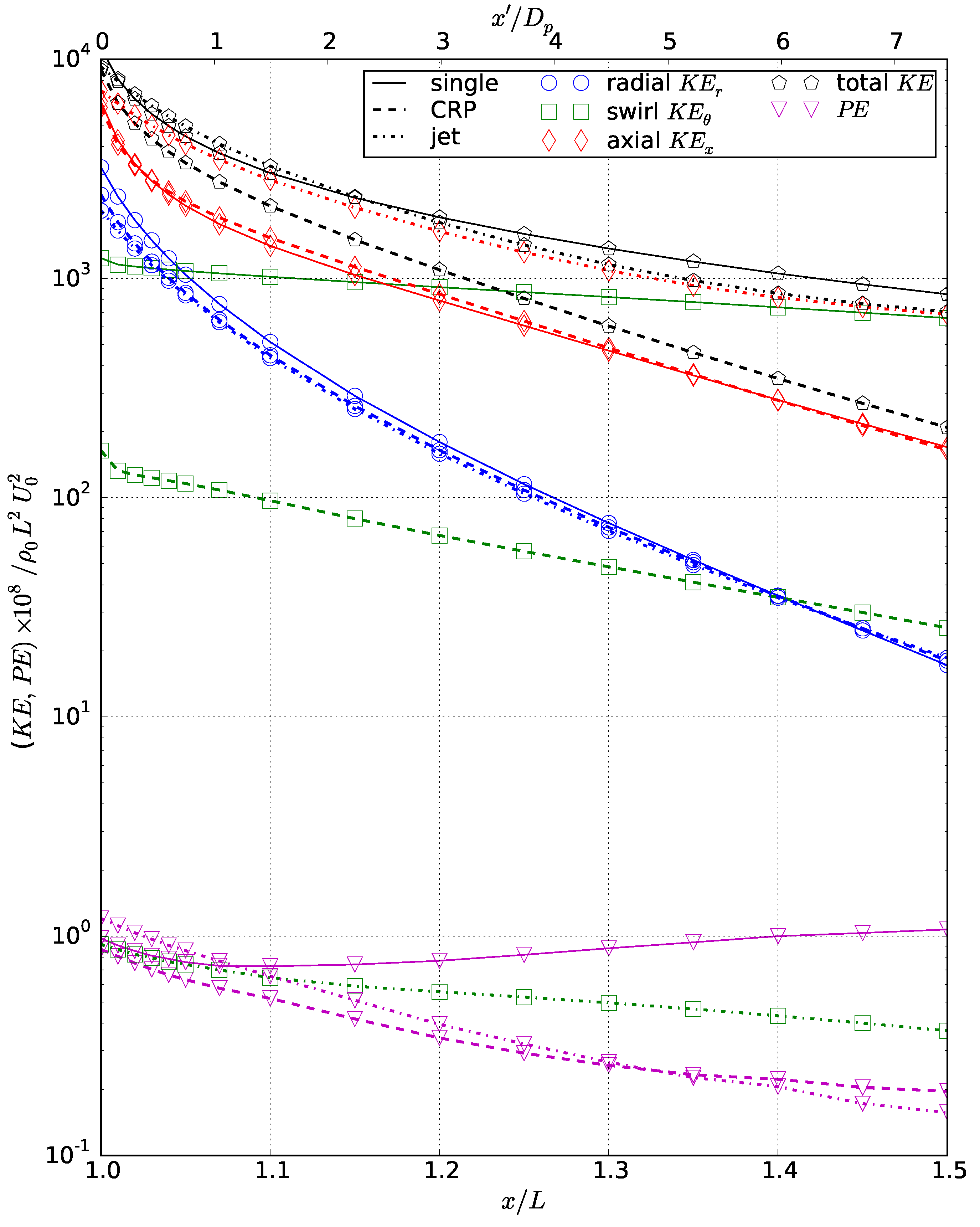
This study examines primary flow variables including: deviation of temperature from the background Δ T and the axial, radial, and azimuthal velocities U x , U r , and U θ , respectively. The second invariant of the velocity gradient tensor Q is computed to visualize vortical structures. The cross-plane-integrated kinetic and potential energies are examined, where the kinetic energy is considered exclusively for each of the three components of velocity K E x , K E r , and K E θ . Data are extracted in axial planes within 0.9755 x / L 1.5 where x is the downstream distance from the bow of the body and L is the body length.

2.10. Flow Coefficients and Case Studies

Several of the important flow coefficients for this propeller-driven flow are the Reynolds number R e L , advance ratio J, thrust coefficient C T , and torque coefficient C Q . An alternate expression for the thrust coefficient C T * is computed for comparison to the jet configuration.
R e L = U 0 L ν , J = U 0 n D p , C T = F T ρ 0 n 2 D P 4 , C T * = F T 1 2 ρ 0 U 0 2 π R 2 , C Q = F Q ρ 0 n 2 D P 5
For these expressions, U 0 is the freestream velocity, ν is kinematic viscosity, D p is the diameter of the propeller, R is the radius of the Iowa Body, n is the propeller speed in revolutions per second, F T is the thrust, and F Q is the torque. The thrust-to-drag ratio is F T / F D . The Reynolds number for this study is R e L = 3.1 × 10 8 , a typical operating condition in the ocean. Other coefficients are listed in Table 4. The fore and aft propellers are listed individually for the CRP case, and total thrust is equivalent for all cases.
The Froude number F r provides a measure of the density stratification, where an infinite F r means zero stratification, and a small F r means high levels of stratification. The present study considers a linearly varying temperature stratification, typical of an ocean environment, with a Froude number of F r = 350 , where,
F r = 1 N U 0 D , and N = 1 2 π g ρ 0 ρ z .
In these expressions N is the Brunt Väisälä frequency, g is acceleration due to gravity, and z is the vertical coordinate. The influence of buoyancy on the near-wake fluid dynamics is often small and can be quantified by the Richardson number R i , which is the ratio of buoyancy to flow gradient terms [15].
R i = g T 0 d T ¯ / d z ( d U ¯ / d z ) 2
where T 0 is a reference temperature, T ¯ is the mean temperature, and U ¯ is the mean velocity. For the single-propeller case, R i 2.54 × 10 3 which indicates that the near-wake inertial forces of the propeller dominate the buoyancy forces. As the local velocity U x decays, R i increases and buoyancy forces become important further downstream in the far wake, beyond the geometric bounds of these simulations.

3. Results

3.1. Near-Wake Transition

Individual vortices are visualized using the second invariant of the velocity gradient tensor Q. Figure 4 shows contour surfaces of the non-dimensionalized ( L / U 0 ) 2 Q = 16.9 with a vertical cutting plane colored by axial velocity defect U x / U 0 1 that extends to half of a body length downstream where x / L = 1.5 . For the single-propeller case, root and tip vortices induced by the propeller are apparent. These vortices follow a helical path and disappear by x / L 1.25 . For the CRP case, additional complexity is introduced by the interaction between the two propellers. Complicated vortical structures are visible until x / L 1.35 . Negligible vortical structures are found in the case of the zero-swirl jet. This figure illustrates the complexity introduced by contra-rotating propellers in comparison to the other two cases.
To better understand the transition from near to far wake regimes in the propeller-driven cases, axial planes behind in the propulsor are examined. Figure 5 compares the instantaneous and time-averaged axial velocity defect field U x / U 0 1 for the single propeller case. Instantaneous fields are taken at an arbitrary time long after initial-transient features have disappeared from the simulation and the flow field has become periodic. Time-averaging occurs over temporal interval of two periods of the propeller. Near the propellers, at x / L = 1.01 and x / L = 1.10 , individual propeller-blade wakes can be seen in the instantaneous field. These blade wakes follow the azimuthal motion of the propellers directly upstream. The time-averaged field, by contrast, is axisymmetric. Further downstream at x / L = 1.3 , only a small variation is seen between the instantaneous and time-averaged fields, and by x / L = 1.45 , the two contour maps are nearly identical showing that the wake is steady and axisymmetric. By half of a body length downstream, the flow is stationary in time and space when viewed from a body-fixed reference frame.
For the CRP case shown in Figure 6, similar observations are drawn. Unsteadiness is apparent for x / L 1.10 , however by x / L = 1.45 the cross-plane profile is temporally stationary. In this case, a unique hexagonal shape is formed due to the interaction between the two opposing three-bladed propellers. This shape is still present at half of a body length downstream of the propulsor.

3.2. Velocity Profiles

The evolution of the near wake may also be described by circumferentially-averaged velocity profiles. Figure 7 shows the circumferentially-averaged velocity defect profiles U x / U 0 for the three self-propelled configurations at the downstream positions x / L = 1.01 , x / L = 1.3 , and x / L = 1.5 . Just behind the propulsor at x / L = 1.01 , the jet is shown to have uniform, positive velocity leaving the exhaust port, while negative velocity due to drag appears for r / R p > 0.2 . By x / L = 1.3 and further at x / L = 1.5 , the jet profile appears as a classical net-zero-momentum wake and may be described using the analytical formulation of the disc-with-center-jet.
Circumferentially averaged profiles of the swirl component of velocity U θ are shown in Figure 8. The jet configuration profile exhibits zero swirl because there are no sources of swirl for this case. The jet exhaust contains uniform axial velocity, the body is axisymmetric, and buoyancy forces are relatively small. The single-propeller configuration at x / L = 1.01 , shows swirl imparted by the propeller and rotating hub. By x / L = 1.3 and x / L = 1.5 , most of the momentum due to swirl exists in a region centered at r / R p 0.4 . In the case of the CRP, regions of positive and negative swirl develop due to interference between the opposing, contra-rotating blades. Throughout the near wake, the CRP swirl magnitude is attenuated, remaining less than half of that of the single propeller, which is explained by the interactions of opposing azimuthal forces of the two propellers.
The propeller-driven cases show their own unique profiles. Positive momentum from the propellers exists in a region near r / R p 0.6 , while negative momentum due to drag from the body exists near the center and further outward. These two circumferentially-averaged profiles are nearly equivalent and decay at similar rates, which is explained by the similar distributions of axial momentum. They also may be defined analytically using a process described in Jones and Paterson [27]. For all configurations, the positive momentum decays more quickly than the negative momentum, which is a feature of idealized wakes described by Tennekes and Lumley [38]. The theoretical, axisymmetric drag wake decays with the power of −2/3, while the theoretical, axisymmetric jet decays with the power of −1.

3.3. Velocity and Temperature Fields in the Mixed-Patch

The wake is mixed by half of a body length downstream of the stern. Unsteadiness from the propulsor has disappeared and axial gradients are small in comparison to the transverse. This location is significant because a cross-plane profile may be considered as the initial data plane (IDP) for further far-wake simulations, which is beyond the scope of this paper. Unique features of the IDP cross-plane profiles of velocity and temperature deviation are presented.

3.3.1. Velocity Field

Cross-plane contour maps of the axial velocity defect U x / U 0 1 at x / L = 1.5 are shown for the single propeller and CRP cases in Figure 9. For the single propeller, axial velocity is axisymmetric and has previously been fit to an analytical curve as a function of radial distance [27]. The CRP, however, is not axisymmetric, and a steady, hexagonal profile is formed. The geometric shape is attributed to the two three-bladed propellers interacting with one another. Unlike the single-propeller profile, the CRP profile is a function of both radial and azimuthal positions. To create an analytical expression as a function of radial position alone, the profile must first be circumferentially averaged.
The swirl component of velocity U θ / U 0 is shown in Figure 10. Again, the single-propeller velocity is axisymmetric, while the CRP velocity has discernible geometry. The magnitude of swirl velocity is much higher for the single propeller case, since the CRP propulsor imparts opposing azimuthal forces. Swirl velocity from the CRP is less than half of that of the single propeller and varies in azimuthal sign.

3.3.2. Temperature Field

Because these simulations take place in a thermally-stratified environment, any vertical redistribution of the fluid will generate potential energy. Mixing in the wake plays an important role in the redistribution of temperature T. Given that the background temperature field T b is initially linearly stratified, mixing from the wake develops a temperature deviation Δ T = T T b . This field is non-dimensionalized by the linear change in temperature over the depth of one propeller-blade length Δ T R p .
Figure 11 shows Δ T / Δ T R p for the single-propeller case. Additional radial profiles help to visualize how the field varies in polar coordinates. A unique cross-plane profile shape is formed that is steady in time. Colder fluid has been driven to the top, while warmer fluid has been driven to the bottom of the wake. A maximum is found near the center of the warm region and a minimum is found near the center of the colder region. Two “tails” are shown trailing off of the warm and cold regions as a result of the counter-clockwise swirling motion of the fluid due to the propeller.
The mixed-patch Δ T / Δ T R p cross-plane profile of the CRP case is shown in Figure 12. Compared to the single-propeller case, the magnitude of Δ T / Δ T R p is less than half. The profile is split between an inner region where clockwise-swirling fluid dominates and an exterior region where counter-clockwise-swirling fluid dominates as shown previously in Figure 8. The complexity and lower Δ T / Δ T R p magnitude in the profile arise directly from the initial interactions of the opposing azimuthal forces of the contra-rotating blades that drive the swirling fluid. While a single propeller can transport the temperature field across the swirling wake region unimpeded, the addition of an opposing propeller directly counters this effect. The net-swirl in the wake is reduced and regions of both positive and negative swirl exist. The inner, negative-swirl region forms a Δ T / Δ T R p profile that mirrors the single-propeller case because of the sign difference in swirl. The outer, positive swirl region shares the same sign of Δ T / Δ T R p as the single-propeller case. In effect, the net loss in swirl reduces the overall potential energy.
Finally, the mixed-patch Δ T / Δ T R p cross-plane profile of the jet case is shown in Figure 13. For this configuration, the magnitude of Δ T / Δ T R p is the smallest due to the absence of swirl. Instead, the shearing of axial momentum and potential effects from the body control the shape of the profile. The positive-momentum “jet” core entrains fluid from the negative-momentum “drag” periphery of the wake. Potential effects from the body further influence the temperature distribution. The resulting transport of Δ T / Δ T R p suspends warmer fluid above colder fluid in the center, and the reverse in sign in the periphery. Without swirl, the distribution of Δ T / Δ T R p in the central core of the jet wake is opposite in sign to that of the single-propeller case.

3.3.3. Comparison to a Perfectly-Mixed Temperature Field

The simulated cross-plane profiles may be compared to the idealized, perfectly-mixed profile shown in Figure 14. This conceptual profile assumes perfect mixing such that the temperature distribution T is uniform up until the boundary of the wake disc, beyond which T = T b . The temperature deviation Δ T = T T b , however, varies because of changes from the background stratification within the disc. Given the linear background stratification, Δ T also varies linearly in the vertical direction. The single propeller case relates most closely to this idealized profile, but, because it does not perfectly-mix T, differences can be observed. The upper and lower regions of colder and warmer fluid are shifted from the centerline, and the maximum temperature deviations are not on the wake boundary but instead closer inward. Results from the single propeller case show that T is not mixed uniformly within the disc of the swirling wake.

3.4. Potential and Kinetic Energy Evolution

Kinetic and potential energy is integrated along axial planes downstream for the three configurations, as shown in Figure 15. Kinetic energy K E is computed individually for the three components of velocity, namely radial, swirl, and axial as K E r , K E θ , and K E x , respectively, as well as for the velocity magnitude, K E . Downstream distance is described both by x / L measured from the bow and by x / D p measured from the stern.
For all three cases, K E r decays more rapidly than K E x and K E θ . The swirl component notably exhibits the slowest decay in the near wake, an observation consistent with Sirviente and Patel [9]. For the single-propeller case, this relative persistence leads to a rise in P E due to expansion of the wake and entrainment of the surrounding passive scalar T, indicating a change in density. For the CRP, the P E does not grow due to the opposing regions of positive and negative swirl velocity. Instead, the P E decays with a rate similar to the zero-swirl jet. This result shows that the contra-rotating blades can effectively reduce P E , which will reduce the strength of buoyancy effects in the far wake.
Comparing the swirl component for the three cases, K E θ of the CRP is an order of magnitude lower than that of the single propeller. Counteracting azimuthal momentum leads to a reduction in the swirl kinetic energy. The reduced K E θ of the CRP is consistent with its reduced P E . The jet K E θ is small because of the initial absence of swirl.
Additionally, comparison of the total K E shows that the CRP is the most-effective configuration for the total reduction of energy by x / L = 1.5 . This increased decay rate suggests that the CRP far wake will decay more quickly than the single propeller and jet cases. The single propeller is less effective than the jet due to persisting K E θ from its unidirectional swirling velocity.

4. Conclusions

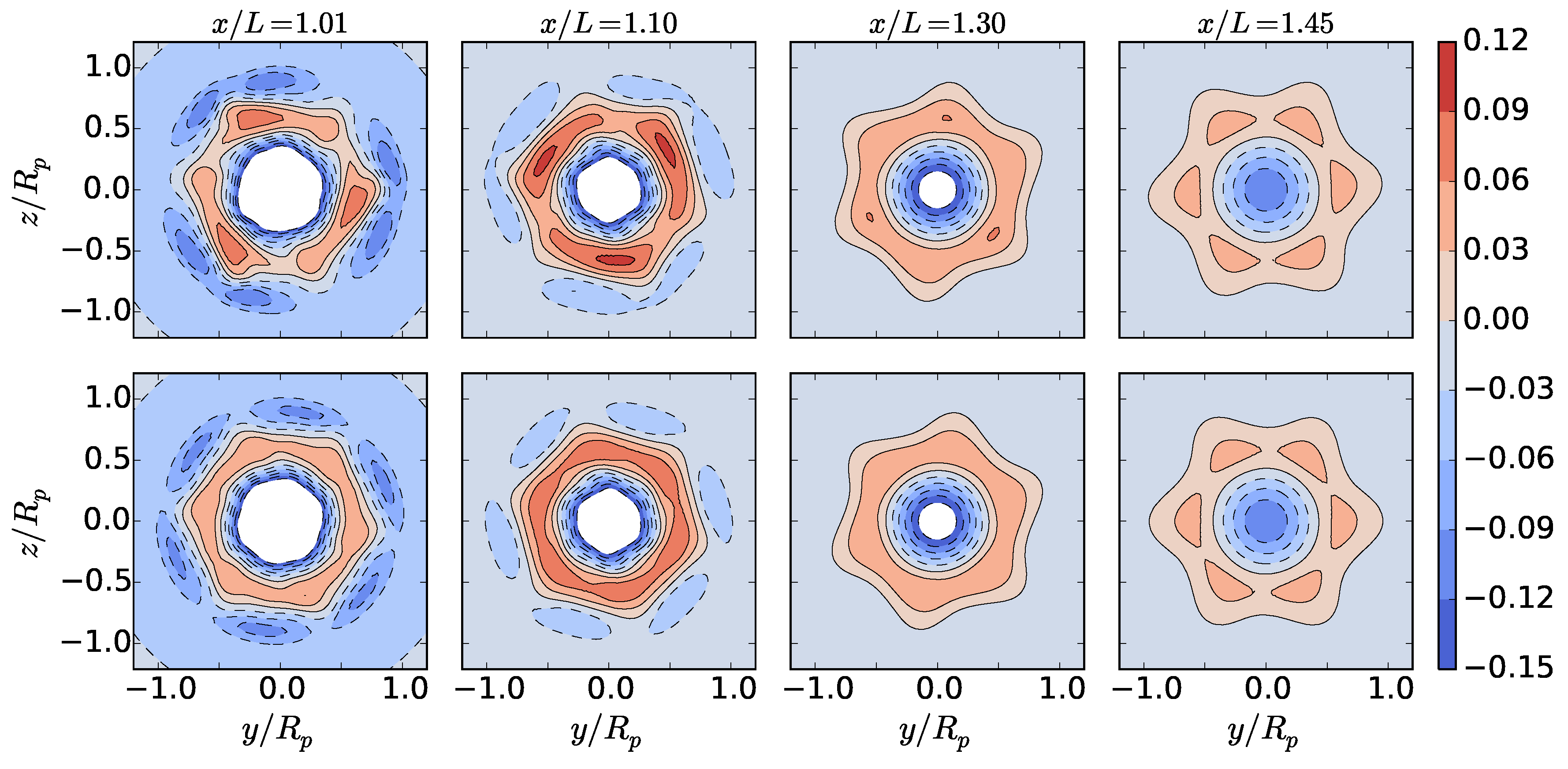
The influence of swirl on the evolution of self-propelled, stratified near wakes and the development of the mixed patch has not previously been well-characterized. In this study, the linearly stratified near wake of the Iowa body was investigated with three separate propulsor configurations: single propeller, contra-rotating propellers, and a zero-swirl, uniform-velocity jet. Unsteady, rotating propeller blades were simulated using an AL model in a URANS computation. Comparison between the configurations revealed unique differences in the evolution of the near wake.
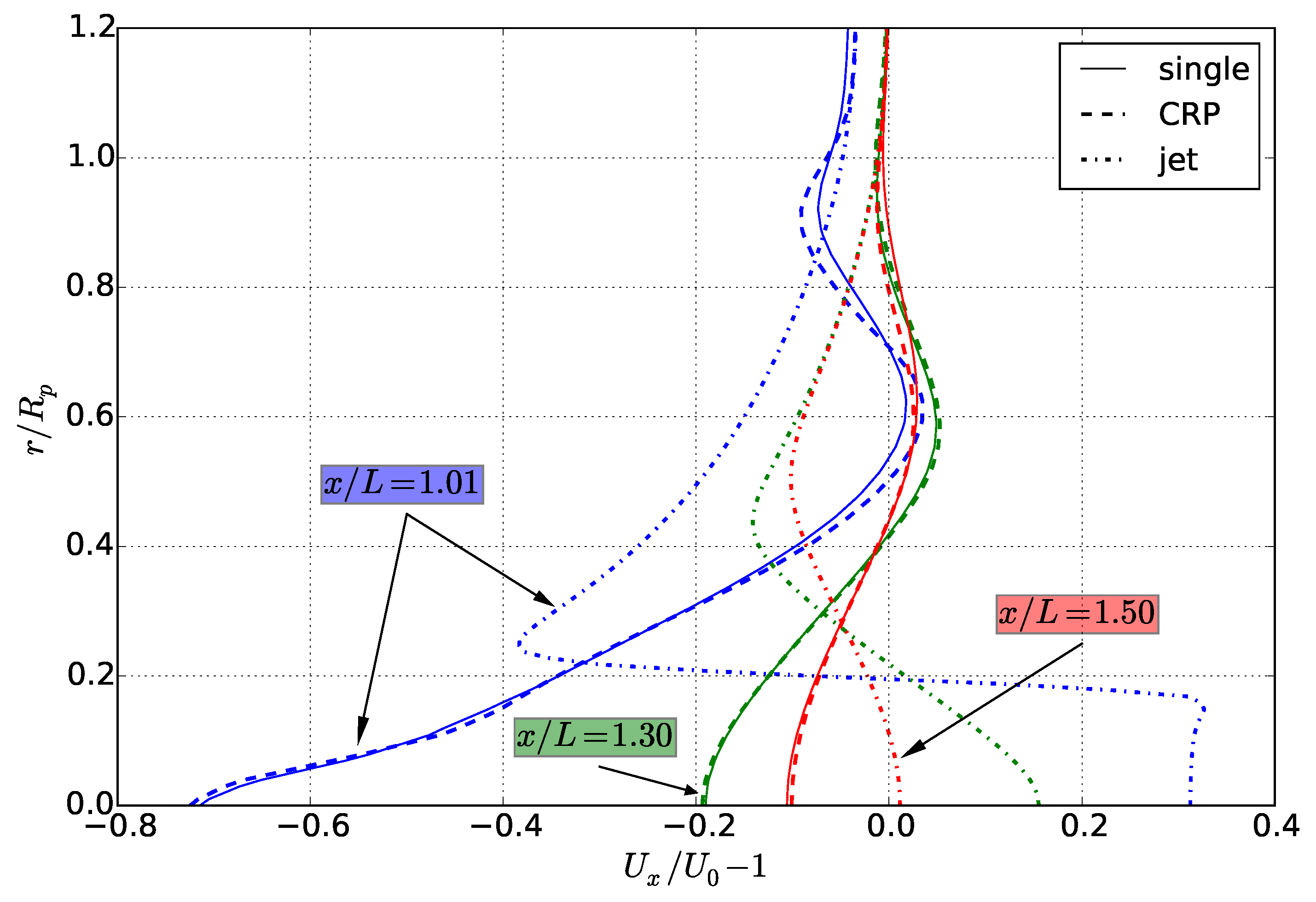
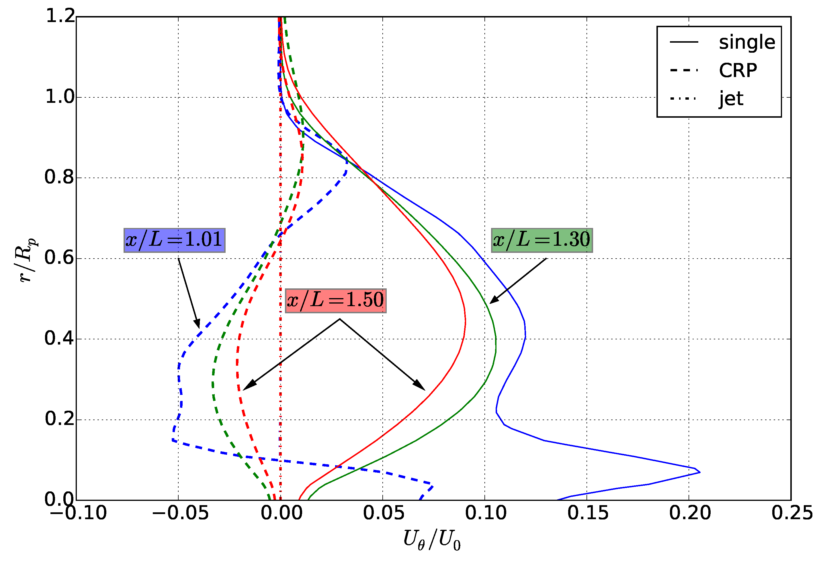
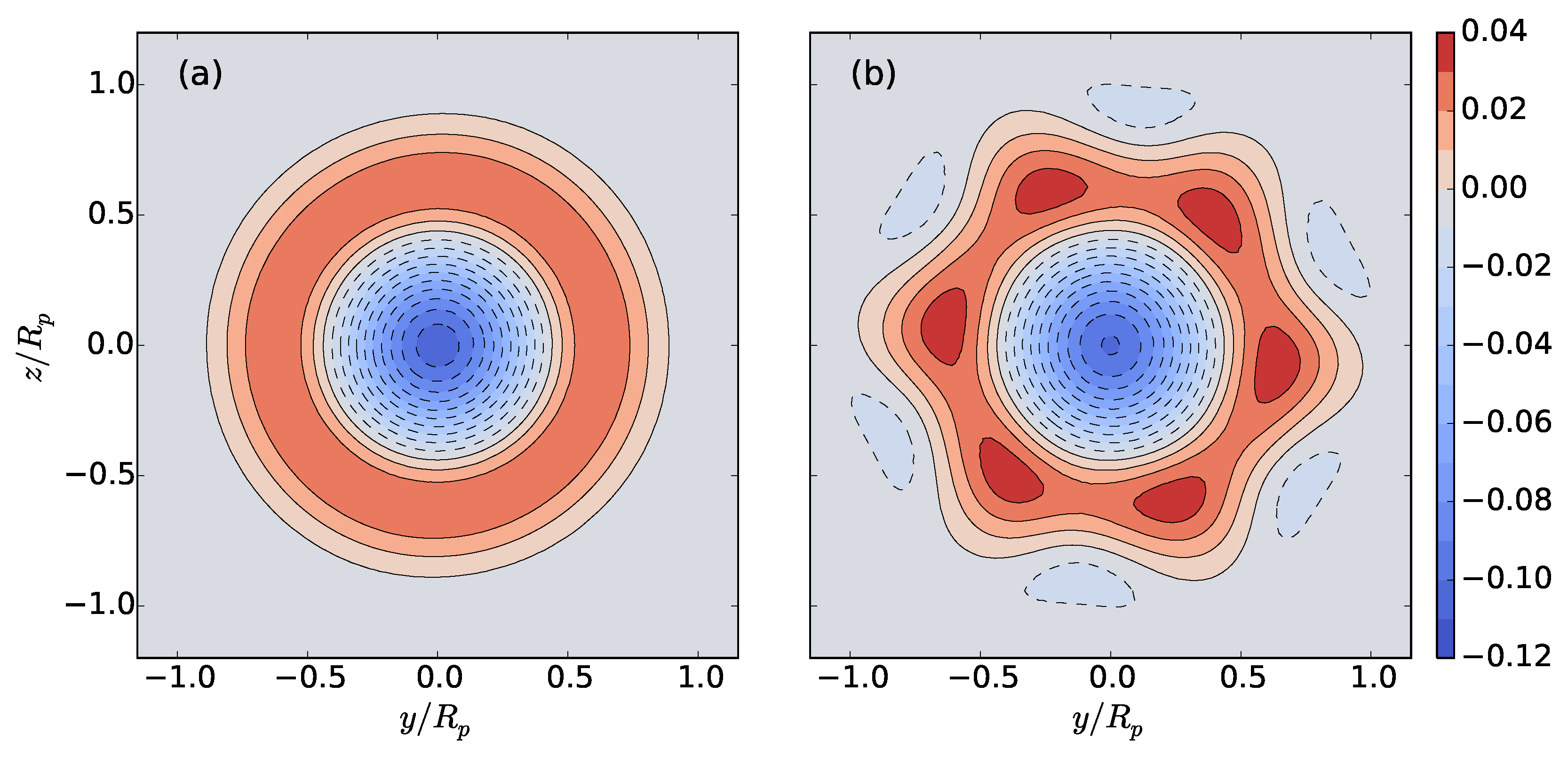
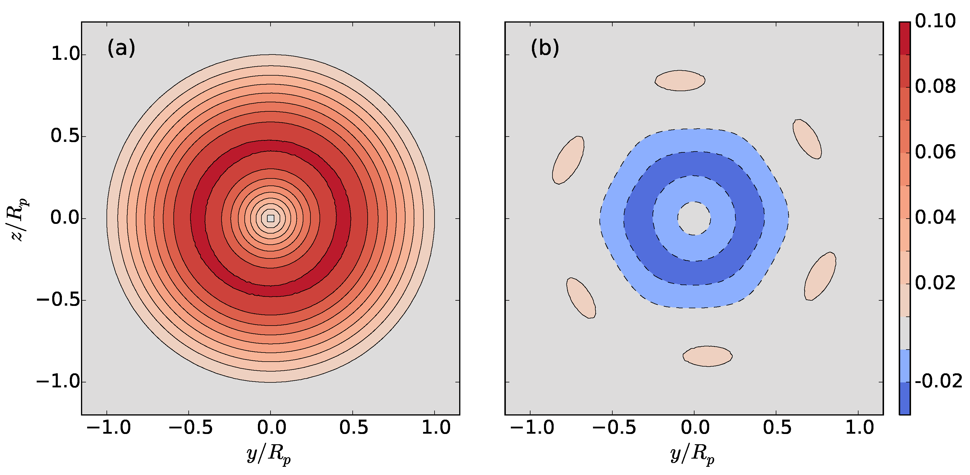
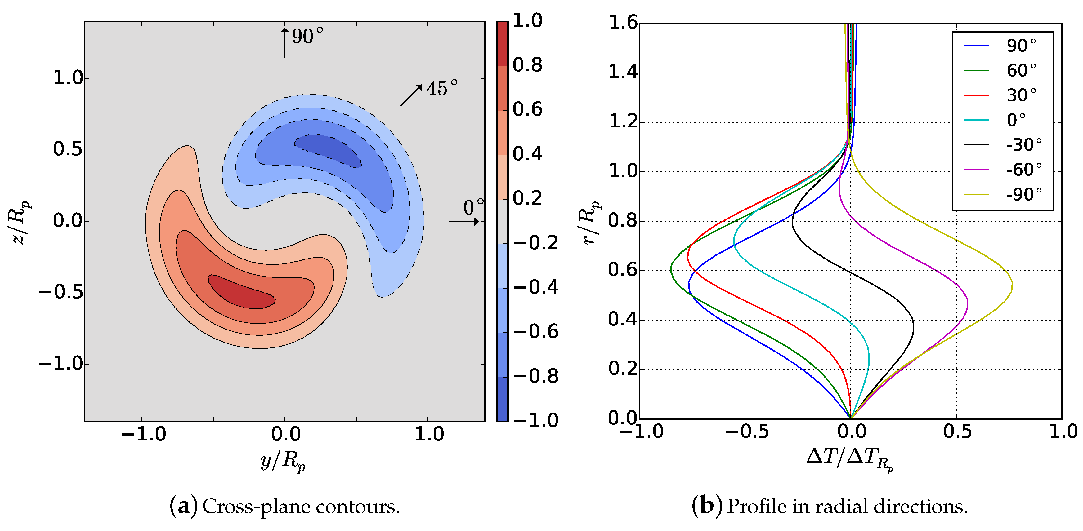
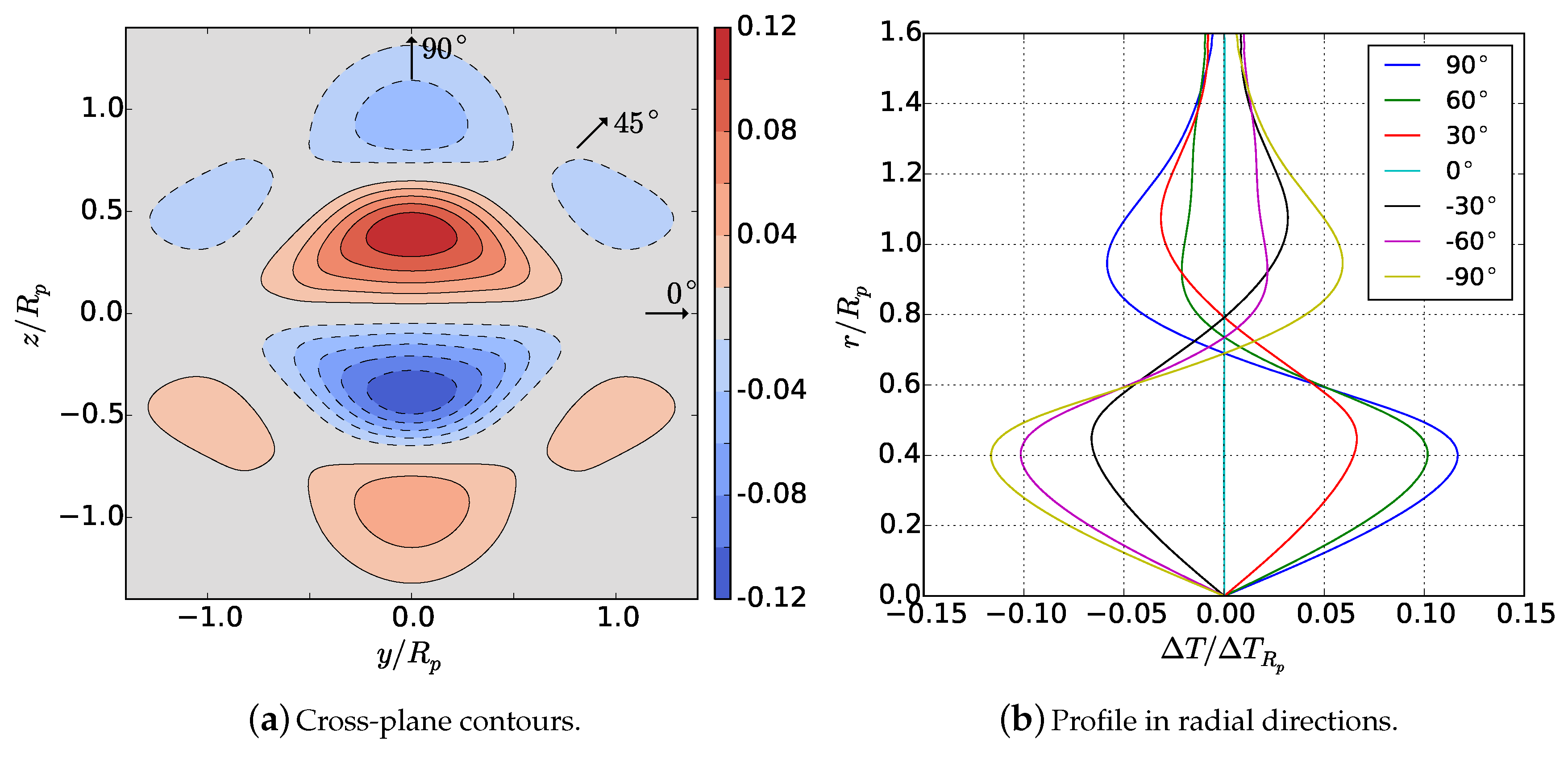
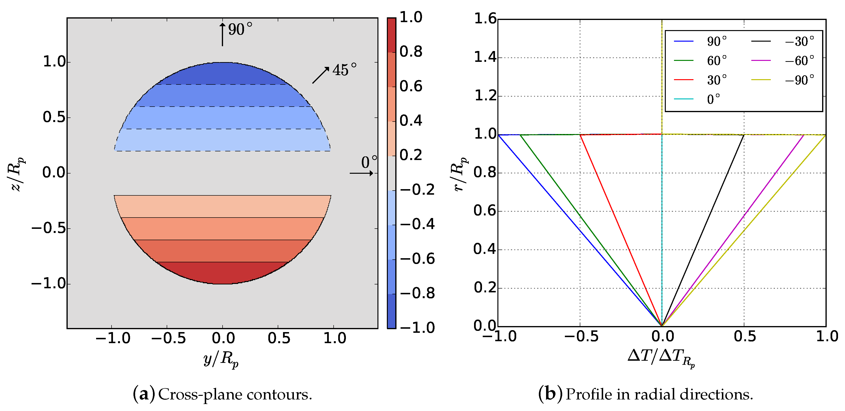
While clear root and tip vortices were visible in the single-propeller case, the CRP disrupted these structures, introducing additional complexity in the wake evolution. Nevertheless, by half of a body length downstream, the wake flow fields were steady in time. The single-propeller and CRP cases shared similar circumferentially-averaged axial velocity defect profiles due to similar spanwise loading in the propulsor. Swirl velocity, however, varied between the two propeller-driven cases, with the CRP introducing both positive and negative swirl regions exhibiting half of the magnitude of the single-propeller case. Furthermore, by half of a body length downstream, the magnitude of the temperature deviation Δ T / Δ T R p for the CRP was less than half of that of the single propeller. The jet Δ T / Δ T R p magnitude was the smallest, due to the absence of swirl. Contour maps of velocity revealed that the single propeller has an axisymmetric profile, whereas the CRP exhibits a unique hexagonal structure as a result of its two three-bladed propellers. The evolution of kinetic and potential energy varied as a direct result of the swirl imparted by each propulsor. Because of the interaction of positive and negative swirl, the CRP configuration showed an order of magnitude lower swirling kinetic energy compared to the single propeller configuration. Additionally, its potential energy was similar in decay and magnitude to that of the swirl-free jet, and the total kinetic energy decayed most rapidly out of the three propulsion schemes. These results indicate that the CRP can effectively reduce potential energy that would otherwise develop from a single-propeller configuration. By removing potential energy, buoyancy effects in the far wake will be weakened.

Author Contributions

Matthew C. Jones implemented the SOWFA actuator-line method into in-house code, conducted and analyzed the simulations, and wrote the paper. Eric G. Paterson is Principal Investigator of the research and dissertation adviser to the first author .

Acknowledgments

The first author has been supported by a Rolls-Royce Commonwealth Graduate Fellowship at Virginia Tech. Virginia Tech Advanced Research Computing is also acknowledged for providing high-performance computing resources. Finally, Matt Churchfield is acknowledged for advising in the implementation of the actuator-line model code from the SOWFA library.

Conflicts of Interest

The authors declare no conflict of interest.

Abbreviations

The following abbreviations are used in this manuscript:
ALActuator line
DNSDirect Numerical Simulation
CRPContra-rotating propeller
SOWFASimulator fOr Wind Farm Applications
URANSunsteady Reynolds-Averaged Navier–Stokes

References

  1. Hyun, B.S. Measurements in the Flow Around a Marine Propeller at the Stern of an Axisymmetric Body. Ph.D. Thesis, University of Iowa, Iowa City, IA, USA, 1990. [Google Scholar]
  2. Hyun, B.S.; Patel, V.C. Measurements in the flow around a marine propeller at the stern of an axisymmetric body. Exp. Fluids 1991, 11, 33–44. [Google Scholar] [CrossRef]
  3. Sirviente, A.; Patel, V.C. Wake of a self-propelled body, part 1: Momentumless wake. AIAA J. 2000, 38, 613–619. [Google Scholar] [CrossRef]
  4. Posa, A.; Balaras, E. A numerical investigation of the wake of an axisymmetric body with appendages. J. Fluid Mech. 2016, 792, 470–498. [Google Scholar] [CrossRef]
  5. Felli, M.; Camussi, R.; Di Felice, F. Mechanisms of evolution of the propeller wake in the transition and far fields. J. Fluid Mech. 2011, 682, 5–53. [Google Scholar] [CrossRef] [Green Version]
  6. Posa, A.; Balaras, E. Large-eddy simulations of a propelled submarine model. In Proceedings of the APS Division of Fluid Dynamics Meeting Abstracts, Boston, MA, USA, 22–24 November 2015. [Google Scholar]
  7. Posa, A.; Balaras, E. Large–eddy simulations of a notional submarine in towed and self–propelled configurations. Comput. Fluids 2018, 165, 116–126. [Google Scholar] [CrossRef]
  8. Lucca-Negro, O.; O’Doherty, T. Vortex breakdown: A review. Progress Energy Combust. Sci. 2001, 27, 431–481. [Google Scholar] [CrossRef]
  9. Sirviente, A.; Patel, V.C. Wake of a self–propelled body, part 2: Momentumless wake with swirl. AIAA J. 2000, 38, 620–627. [Google Scholar] [CrossRef]
  10. Esmaeilpour, M.; Martin, J.E.; Carrica, P.M. Near-field flow of submarines and ships advancing in a stable stratified fluid. Ocean Eng. 2016, 123, 75–95. [Google Scholar] [CrossRef]
  11. Hassid, S. Collapse of turbulent wakes in stably stratified media. J. Hydronaut. 1980, 14, 25–32. [Google Scholar] [CrossRef]
  12. Chernykh, G.; Voropayeva, O. Numerical modeling of momentumless turbulent wake dynamics in a linearly stratified medium. Comput. Fluids 1999, 28, 281–306. [Google Scholar] [CrossRef]
  13. Meunier, P.; Spedding, G.R. Stratified propelled wakes. J. Fluid Mech. 2006, 552, 229–256. [Google Scholar] [CrossRef]
  14. Brucker, K.A.; Sarkar, S. A comparative study of self–propelled and towed wakes in a stratified fluid. J. Fluid Mech. 2010, 652, 373–404. [Google Scholar] [CrossRef]
  15. Lin, J.; Pao, Y.H. Wakes in stratified fluids. Ann. Rev. Fluid Mech. 1979, 11, 317–338. [Google Scholar] [CrossRef]
  16. Spedding, G. Wake signature detection. Ann. Rev. Fluid Mech. 2013, 46, 273–302. [Google Scholar] [CrossRef]
  17. Pal, A.; de Stadler, M.B.; Sarkar, S. The spatial evolution of fluctuations in a self–propelled wake compared to a patch of turbulence. Phys. Fluids 2013, 25, 095106. [Google Scholar] [CrossRef]
  18. Pal, A. Dynamics of Stratified Flow Past a Sphere: Simulations Using Temporal, Spatial and Body Inclusive Numerical Models; University of California: San Diego, CA, USA, 2016. [Google Scholar]
  19. Pal, A.; Sarkar, S. Effect of external turbulence on the evolution of a wake in stratified and unstratified environments. J. Fluid Mech. 2015, 772, 361–385. [Google Scholar] [CrossRef]
  20. De Stadler, M.B.; Sarkar, S. Simulation of a propelled wake with moderate excess momentum in a stratified fluid. J. Fluid Mech. 2012, 692, 28–52. [Google Scholar] [CrossRef]
  21. Spedding, G. The evolution of initially turbulent bluff–body wakes at high internal Froude number. J. Fluid Mech. 1997, 337, 283–301. [Google Scholar] [CrossRef]
  22. Pal, A.; Sarkar, S.; Posa, A.; Balaras, E. Direct numerical simulation of stratified flow past a sphere at a subcritical reynolds number of 3700 and moderate froude number. J. Fluid Mech. 2017, 826, 5–31. [Google Scholar] [CrossRef]
  23. Naudascher, E. Flow in the wake of self–propelled bodies and related sources of turbulence. J. Fluid Mech. 1965, 22, 625–656. [Google Scholar] [CrossRef]
  24. Lin, J.; Pao, Y. Velocity and Density Measurements in the Turbulent Wake of a Propeller-Driven Slender Body in a Stratified Fluid; Flow Research Inc.: Middlesex, MA, USA, 1974. [Google Scholar]
  25. Schetz, J.; Jakubowski, A. Experimental studies of the turbulent wake behind self–propelled slender bodies. AIAA J. 1975, 13, 1568–1575. [Google Scholar] [CrossRef]
  26. Sanderse, B.; Pijl, S.; Koren, B. Review of computational fluid dynamics for wind turbine wake aerodynamics. Wind Energy 2011, 14, 799–819. [Google Scholar] [CrossRef]
  27. Jones, M.C.; Paterson, E.G. Evolution of the propeller near-wake and potential energy in a thermally- stratified environment. In Proceedings of the OCEANS 2016 MTS/IEEE Monterey, Monterey, CA, USA, 19–23 September 2016; pp. 1–10. [Google Scholar]
  28. Jones, M.C.; Paterson, E.G. Influence of propulsion type on the near-wake evolution of kinetic and potential energy. In Proceedings of the Fifth International Symposium on Marine Propulsors, Helsinki, Finland, 12–15 June 2017; pp. 1–8. [Google Scholar]
  29. Menter, F.R. Two-equation eddy-viscosity turbulence models for engineering applications. AIAA J. 1994, 32, 1598–1605. [Google Scholar] [CrossRef]
  30. Fofonoff, N.P.; Millard, R.C. Algorithms for computation of fundamental properties of seawater. UNESCO Tech. Pap. Mar. Sci. 1983, 44, 1–53. [Google Scholar]
  31. Holliday, D.; McIntyre, M.E. On potential energy density in an incompressible, stratified fluid. J. Fluid Mech. 1981, 107, 221–225. [Google Scholar] [CrossRef]
  32. NWTC Information Portal (SOWFA). Available online: https://nwtc.nrel.gov/SOWFA (accessed on 21 April 2016).
  33. Troldborg, N. Actuator Line Modeling of Wind Turbine Wakes. Ph.D. Thesis, Technical University of Denmark, Lyngby, Denmark, 2008. [Google Scholar]
  34. Martınez, L.A.; Leonardi, S.; Churchfield, M.J.; Moriarty, P.J. A comparison of actuator disk and actuator line wind turbine models and best practices for their use. In Proceedings of the 50th AIAA Aerospace Sciences Meeting including the New Horizons Forum and Aerospace Exposition, Nashville, TN, USA, 9–12 January 2012. [Google Scholar]
  35. Brockett, T. Minimum Pressure Envelopes for Modified Naca-66 Sections with Naca a = 0.8 Camber and Buships Type 1 and Type 2 Sections; Technical Report; DTIC Document: Fort Belvoir, VA, USA, 1966. [Google Scholar]
  36. cfMesh 1.1.1. Available online: http://www.cfmesh.com/ (accessed on 16 February 2016).
  37. Issa, R.I. Solution of the implicitly discretised fluid flow equations by operator-splitting. J. Comput. Phys. 1986, 62, 40–65. [Google Scholar] [CrossRef]
  38. Tennekes, H.; Lumley, J.L. A First Course in Turbulence; MIT Press: Cambridge, MA, USA, 1972. [Google Scholar]
Figure 1. Non-dimensional body force on mesh slice at propeller plane | f p | / ( ρ 0 R p rps 2 ) for the single-propeller case.
Jmse 06 00046 g001
Figure 2. Standard Iowa Body profile.
Jmse 06 00046 g002
Figure 3. Computational meshes generated for each configuration.
Jmse 06 00046 g003
Figure 4. Flow visualization for x/L ≤ 1.5 using Q-criterion visualization non-dimensionalized as (L/U0)2Q = 16.9 colored by Ux/U0 − 1 with vertical cutting plane through mesh.
Jmse 06 00046 g004
Figure 5. Instantaneous (top); and time-averaged (bottom) velocity defect U x / U 0 1 for the single propeller case.
Jmse 06 00046 g005
Figure 6. Instantaneous (top); and time-averaged (bottom) velocity defect U x / U 0 1 for the CRP case.
Jmse 06 00046 g006
Figure 7. Circumferentially-averaged velocity defect U x / U 0 1 profiles for each configuration at various distances downstream.
Jmse 06 00046 g007
Figure 8. Circumferentially-averaged swirl velocity U θ / U 0 profiles for each configuration at various distances downstream.
Jmse 06 00046 g008
Figure 9. Velocity defect U x / U 0 1 profiles at x / L = 1.5 for single propeller (a) and CRP (b) cases.
Jmse 06 00046 g009
Figure 10. Swirl velocity U θ / U 0 profiles at x / L = 1.5 for single propeller (a) and CRP (b) cases.
Jmse 06 00046 g010
Figure 11. Single propeller ΔTTRp at x/L = 1.5.
Jmse 06 00046 g011
Figure 12. CRP ΔTTRp at x/L = 1.5.
Jmse 06 00046 g012
Figure 13. Jet configuration ΔTTRp at x/L = 1.5.
Jmse 06 00046 g013
Figure 14. Idealized mixed-patch profile of ΔTTRp for a wake region of constant T.
Jmse 06 00046 g014
Figure 15. Integrated energy evolution downstream of the vehicle for each configuration, with x measured from the bow of the hull and x measured from the stern.
Jmse 06 00046 g015
Table 1. Coefficients in UNESCO equation of state for seawater.
CoefficientValueCoefficientValueCoefficientValue
a 0 9.998425 × 10 2 b 0 8.2449 × 10 1 c 0 5.7247 × 10 3
a 1 6.793952 × 10 2 b 1 4.0899 × 10 3 c 1 1.0227 × 10 4
a 2 9.095290 × 10 3 b 2 7.6438 × 10 5 c 2 1.6546 × 10 6
a 3 1.001685 × 10 4 b 3 8.2467 × 10 7 d 0 4.8314 × 10 4
a 4 1.120083 × 10 6 b 4 5.3875 × 10 9
a 5 6.536332 × 10 9
Table 2. Iowa Body geometry.
FeatureValue
L / D 10.90
D / D p 1.369
D p / D h 6.266
Hub location 0.9688 < x / L < 0.9832
Propeller location x / L = 0.9755
Number of blades3
Propeller hydrofoilNACA 66-Modified
Table 3. Mesh design and quality features.
Mesh FeatureValue
Boundary layer cells > 20
Near-wall mesh spacing y + < 100
Propulsor and wake cells/ D p 100
Wake region extends to x / L = 1.6
Total number of cells 2 × 10 7
Maximum aspect ratio AR < 170
Maximum non-orthogonality < 45
Maximum skewness < 0.8
Table 4. Flow coefficients.
ConfigurationJ C T C T * C Q F T / F D
Single0.860.0470.0840.0110.99
CRP (fore)0.900.0240.0410.00710.50
CRP (aft)0.860.0230.0410.00720.50
Jet--0.08201.07

