Article

Prediction of the Open-Water Performance of Ducted Propellers with a Panel Method

by
João Manuel Baltazar
1,*,
Douwe Rijpkema
2,
José Falcão de Campos
1 and
Johan Bosschers
2
1
Department of Mechanical Engineering, Instituto Superior Técnico, Av. Rovisco Pais 1, Universidade de Lisboa, 1049-001 Lisboa, Portugal
2
Maritime Research Institute Netherlands, 2 Haagsteeg, 6708 PM Wageningen, The Netherlands
*
Author to whom correspondence should be addressed.
J. Mar. Sci. Eng. 2018, 6(1), 27; https://doi.org/10.3390/jmse6010027
Submission received: 16 January 2018 / Revised: 21 February 2018 / Accepted: 11 March 2018 / Published: 19 March 2018
(This article belongs to the Special Issue Marine Propulsors)

Abstract

:
In the present work, a comparison between the results obtained by a panel code with a Reynolds-averaged Navier-Stokes (RANS) code is made to obtain a better insight on the viscous effects of the ducted propeller and on the limitations of the inviscid flow model, especially near bollard pull conditions or low advance ratios, which are important in the design stage. The analysis is carried out for propeller Ka4-70 operating inside duct 19A. From the comparison, several modelling aspects are studied for improvement of the inviscid (potential) flow solution. Finally, the experimental open-water data is compared with the panel method and RANS solutions. A strong influence of the blade wake pitch, especially near the blade tip, on the ducted propeller force predictions is seen. A reduction of the pitch of the gap strip is proposed for improvement of the performance prediction at low advance ratios.

1. Introduction

In recent years, substantial progress is being made in the computation of the flow around ducted propeller systems with Reynolds-averaged Navier-Stokes (RANS) equations by several research groups. For example, Sánchez-Caja et al. [1] used a RANS solver to simulate incompressible viscous flow around a propeller in the presence of a duct. Posteriorly, the influence of the rudder was also taken into account in the calculation of the viscous flow [2]. In addition, Abdel-Maksoud and Heinke [3], and Bhattacharyya et al. [4] have investigated the scale effects on ducted propellers numerically using RANS. Alternatively, Kim et al. [5] presented detailed RANS simulations for a ducted propeller system including verification and validation studies. Subvisual cavitation and acoustics modelling were also investigated in this work. However, the computational effort is still reasonably high due to the need for good numerical resolution in small flow regions dominated by strong viscous effects such as in the gap between the propeller blade tip and duct. This requirement poses considerable demands in the number of grid cells needed for accurate computations with associated long computational times, which still makes the method less useful for routine design studies.
On the other hand, in the past a number of methods based on inviscid potential flow theory have been proposed for the analysis of ducted propellers. Kerwin et al. [6] combined a panel method for the duct with a vortex lattice method for the propeller. This method was compared with experimental data available from open-water tests by Hughes et al. [7]. Later, Hughes [8] presented a complete three-dimensional panel method for both the propeller and duct, where a special procedure for modelling the gap flow is implemented. More recently, Lee and Kinnas [9] described a panel method for the unsteady flow analysis of ducted propeller with blade sheet cavitation. These methods are nowadays very efficient from the computational point of view which makes them particularly suited for design studies.
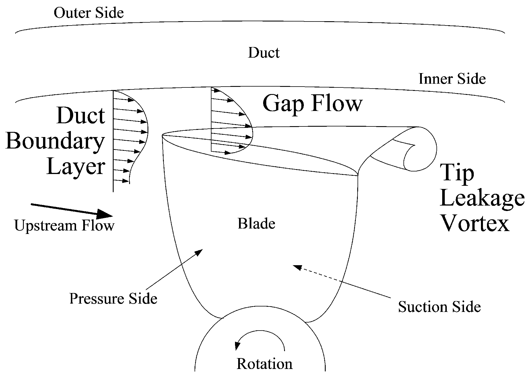
However, the inviscid methods have met serious limitations in their practical applications related to their inability to adequately model viscous effects occurring in a ducted propeller system, especially in the gap region and in the duct boundary layer leading to separation phenomenon. Due to the relative motion between the duct and the propeller blades, combined with the pressure difference across the gap, different viscous mechanisms occur simultaneously in this region, such as the tip-leakage vortex and the gap flow due to the duct and blade boundary layers. Schematics of this process are shown in Figure 1. The flow in the gap region is rather complex, since the duct and blade boundary layers influence the gap flow and consequently the characteristics of the tip-leakage vortex. The tip-leakage vortex is also responsible for the different loading of the ducted propeller in comparison with the open propeller and must be taken into account in the inviscid model. An extensive experimental investigation to examine the tip-leakage flow on ducted propulsors was carried out by Oweis et al. [10]. Another important viscous effect is the flow over the surface of the duct, where separation of the boundary layer creating a recirculation region may occur due to the thick blunt trailing-edge, which also affects the duct loading.
The calculation of the flow around a ducted propeller system in open-water with a panel code has been the subject of investigation by Instituto Superior Técnico (IST) and Maritime Research Institute Netherlands (MARIN), see [11,12,13]. In these studies, a low-order panel method has been used to predict the open-water diagram of a ducted propeller system, where several modelling aspects have been analysed for the improvement of the inviscid (potential) flow solution. The investigation comprehended the influence of the Kutta condition, gap flow model and wake model on the performance prediction. A similar method has also been implemented by MARIN in an in-house panel code [14,15].
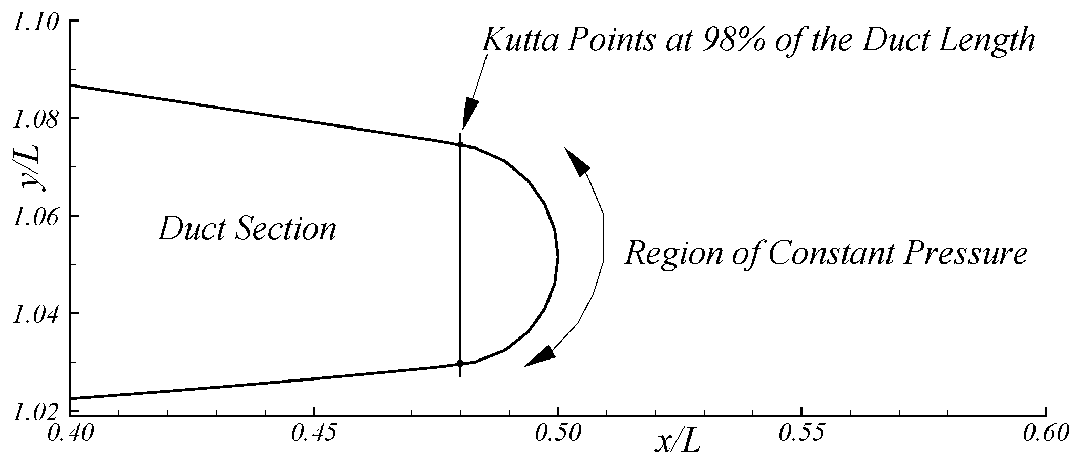
In this investigation, an alternative Kutta condition has been proposed for the duct trailing-edge, which has a thick round geometry in comparison to the sharp trailing-edge of the propeller blades. In this new Kutta condition, the chordwise location for pressure equality on both sides of the duct trailing-edge has a strong influence on the propeller and duct force predictions.
To account for the gap flow between the blade tip and duct inner side, Hughes [8] proposed an iterative procedure where the gap flow is treated as a two-dimensional orifice. In his model, the gap between the blade tip and the duct inner surface is modelled as a rigid surface, named in this study as the gap strip. Then, transpiration velocities are computed from the pressure-difference in the gap strip, where an empirical discharge coefficient is used to take into account the loss of energy as the fluid passes through the gap. A similar gap model has been combined with a vortex-lattice method by Gu and Kinnas [16]. From previous comparative studies, see [11,13], similar results were found between the closed (sealed) gap model and the gap flow model with transpiration velocity based in the work of Hughes [8]. Therefore, the closed gap model is usually preferred in potential flow methods [13,15,17], since a negligible effect on the overall performance is obtained.
The influence of the blade wake geometry on the prediction of the ducted propeller performance with a panel method has been studied in detail, see [11,13]. In this work, the blade wake pitch is aligned with the local flow velocity using an Euler scheme, leading to an improvement in the prediction of the propeller forces. A similar model for alignment of the blade wake was presented by Kinnas et al. [17], and Kim et al. [18] extended the wake alignment scheme for both the blade wake and duct wake. However, from the work carried out by IST and MARIN [11], the loading predictions of the ducted propeller system were found to be critically dependent on the blade wake pitch especially at the tip. In this way, a simple model for the interaction between the blade wake and the boundary layer on the duct inner side was implemented in combination with the wake alignment model [11,13]. With this model, a reasonable to good agreement was obtained between the inviscid predictions and the experimental data from open-water tests [13]. However, significant differences were still seen in the open-water predictions at low advance ratios.
It is known that the prediction of the propeller performance at bollard pull conditions is important in the design stage. In the present work, a comparison between the results obtained by the panel method with RANS calculations is made to obtain a better insight on the viscous effects of the ducted propeller and on the limitations of the inviscid flow model. The comparison focuses mainly at the low advance ratios, where a new approach for the gap strip is proposed in the panel method. The paper is organised as follows: a description of the numerical methods is given in Section 2; the comparison of the inviscid predictions with the RANS calculations and the experimental open-water data is presented in Section 3; in Section 4 the main conclusions are drawn.

2. Numerical Methods

2.1. Problem Definition

Let us consider a propeller of radius R with a finite number of blades symmetrically distributed around an axisymmetric hub, rotating with constant angular velocity Ω inside a duct and advancing with constant axial speed U along its axis. The duct is also considered to be axisymmetric of inner radius at the propeller plane R d > R which defines a gap height h = R d R .
We introduce a Cartesian coordinate system ( x , y , z ) rotating with the propeller blades, with the x-axis positive downstream, the y-axis direction coincident with the propeller reference line, and the z-axis completing the right-hand-system. In this rotating reference frame the flow field is steady. We will use a cylindrical coordinate system ( x , r , θ ) which is related to the Cartesian system by the transformation
y = r cos θ , z = r sin θ .
The undisturbed inflow velocity in the rotating frame is
U = U e x + Ω r e θ ,
where ( e x , e r , e θ ) are the unit vectors of the cylindrical coordinate system. Figure 2 shows the coordinate systems used to describe the geometry and the fluid domain around the ducted propeller.

2.2. Panel Code PROPAN

Assuming an incompressible, ideal and irrotational flow at an infinity domain in all directions, the flow around the ducted propeller can be treated with a potential flow model. PROPAN is a IST in-house code which implements a low-order potential-based panel method for the calculation of the incompressible potential flow around marine propellers. The code has been widely used in the calculation of the three-dimensional potential flow around ducted propellers, [11,13,19].
Applying Green’s second identity and using the so-called Morino formulation [20], which assumes that the perturbation potential is zero in interior region to the blade surfaces S B , duct surface S D and hub surface S H , we obtain the integral representation of the perturbation potential ϕ at a point p on the body surface,
2 π ϕ p = S B S D S H ϕ q n q 1 R ( p , q ) ϕ n q 1 R ( p , q ) d S + S W Δ ϕ q n q 1 R ( p , q ) d S , p S B S D S H ,
where R p , q is the distance between the field point p and the point q on the boundary S B S D S H S W . The perturbation potential must satisfy the Neumann boundary condition at the body surface,
ϕ n n · ϕ = n · U on S B S D S H ,
where / n denotes differentiation along the normal and n is the unit vector normal to the surface directed outward from the body. Equation (3) is a Fredholm integral equation of the second kind in the dipole distribution μ ( q ) = ϕ ( q ) on the surfaces S B , S D and S H . The Kutta condition yields the additional relationship to determine the dipole strength Δ ϕ ( q ) in the wake surfaces S W .
For the numerical solution of Equation (3), we discretise the body surfaces S B , S D and S H , and the wake surfaces S W in bi-linear quadrilateral elements which are defined by four points on the surface. We assume a constant strength of the dipole and source distributions on each element. In the numerical solution of the integral equation, Equation (3), the integrals over the body and wake surfaces are approximated by the summation of the integrals on the elements discretising the surfaces. The element integrals are calculated analytically following the formulation of Morino and Kuo [20].
To determine the dipole strength on the wake surfaces, an iterative pressure Kutta condition at the blade and duct trailing edges is applied. However, different forms of the Kutta condition are considered, since the blade trailing-edge has a sharp geometry, whereas the duct trailing-edge presents a blunt round geometry. For the blade trailing-edge, equal pressure on the collocation points of the panels adjacent to the trailing-edge on the upper and lower sides is considered. For the duct trailing-edge, the chordwise location of pressure equality on both sides is specified, which controls the strength of the shed vorticity. Due to the possible occurrence of flow separation, a constant pressure distribution downstream of the Kutta points is assumed in this model. Note that the potential flow solution at the duct trailing edge satisfies the integral equation, Equation (3), but the corresponding pressure distribution is disregarded aft the Kutta points. A schematic drawing of the pressure Kutta condition for a thick round trailing edge is shown in Figure 3. A detailed description of the iterative method for solution of the pressure Kutta condition may be found in [19].
For the wake geometry, two wake models are considered: a rigid wake model (RWM) and a wake alignment model (WAM). In the rigid wake model, the geometry of the wake surfaces is specified empirically. For the blade wake, the pitch of the vortex lines is assumed constant along the axial direction and equal to the blade pitch. For the duct, the wake leaves the trailing edge at the bisector with constant radius. In the wake alignment model, the blade wake pitch is aligned with the local fluid velocity, while the radial position of the vortex lines is fully prescribed. The new axial x i + 1 ( n + 1 ) and circumferential θ i + 1 ( n + 1 ) coordinates of the wake strip i + 1 at the ( n + 1 ) th iteration are determined by using an Euler scheme:
x i + 1 ( n + 1 ) = x i ( n ) + V x x i ( n ) , r i ( n ) , θ i ( n ) Δ t θ i + 1 ( n + 1 ) = θ i ( n ) + V θ x i ( n ) , r i ( n ) , θ i ( n ) V θ x i ( n ) , r i ( n ) , θ i ( n ) r i ( n ) r i ( n ) Δ t ,
where V x and V θ are the components of the mean vortex sheet velocity along the axial and circumferential directions, respectively, and Δ t is the pseudo-time step for the Euler vortex convection scheme. The velocity components are calculated from the integral equation of the velocity, obtained by taking the gradient of Equation (3). For the time discretisation, an angular time step Δ θ = Ω Δ t is introduced, which can also be expressed in terms of the number of time steps per propeller revolution N θ = 2 π / Δ θ . To account for the interaction between the blade wake and the duct boundary layer on the inner side, see Figure 1, a correction to the blade wake pitch near the tip is introduced in the wake alignment model, whereas a reduction in the axial velocity is taken into account in the convection of the vorticity generated by the blade. Considering δ as the duct boundary layer thickness and assuming a power law distribution for the velocity profile, we have
V x R d r V x δ = R d r δ 1 n .
From Equation (6) the velocity deficit in the axial direction due to the duct boundary layer is taken into account in the wake alignment model, introducing a reduction in the pitch of the blade wake geometry near the tip. However, to avoid zero axial velocity at the duct inner surface in the wake alignment model, which would cause zero pitch for the tip vortex line and a mismatch with the duct grid, a linear variation of the axial velocity is considered in the gap region ( R r R d ) . The corrected axial velocity at the duct surface V x ( 0 ) is obtained by linear extrapolation from the axial velocity at the gap V x ( h ) , and at the edge of the duct boundary layer V x ( δ ) . This correction is applied along the entire length of the blade wake sheet.
The gap between the blade tip and the duct inner surface is modelled as a rigid surface, named in this study as the gap strip, and where the transpiration velocity is neglected. In this closed gap model, the boundary condition on the gap panels sets the source strength to cancel the normal component of the inflow velocity leading to the Neumann boundary condition, Equation (4). The gap strip extends from the blade tip to the duct inner side.

2.3. RANS Code ReFRESCO

Alternatively, in order to address the viscous effects a RANS solver can be used for the simulation of the incompressible viscous flow around ducted propellers. In the present study RANS code ReFRESCO version 2.1 is considered. ReFRESCO (www.refresco.org) is a community-based open-usage CFD code for the maritime world [21] and is currently being developed within a cooperation led by MARIN. It solves the steady incompressible RANS equations, complemented with turbulence models. The time-averaged continuity and momentum equations (RANS equations) written in the differential form and using the tensor notation are:
V i x i = 0 , ρ V j V i x j = p x i + x j μ V i x j + V j x i + τ i j x j ,
where x i ( x 1 , x 2 , x 3 ) are the coordinates of the reference system ( x , y , z ) , V i are the components of the mean velocity vector, ρ the fluid density, p the fluid static pressure, μ the fluid viscosity and τ i j are the Reynolds stresses produced by the averaging process of the momentum equations. In this work, the selected turbulence model is based on the Boussinesq eddy-viscosity hypothesis that determines the Reynolds stresses from
τ i j = μ t V i x j + V j x i 2 3 ρ k δ i j ,
where μ t is the eddy-viscosity, δ i j is the Kronecker symbol and k is the turbulence kinetic energy. For all RANS calculations presented in this paper, the k ω SST two-equation eddy-viscosity turbulence model proposed by Menter et al. [22] is used. In this model, two transport equations are solved: the turbulent kinetic energy k and the specific turbulent dissipation rate ω .
The equations are discretised using a face-based finite-volume approach with cell-centred collocation variables. A strong-conservation form and a pressure-correction equation based on the SIMPLE algorithm is used to ensure mass conservation. For open-water (steady) calculations the equations are solved in the body-fixed reference frame which is rotating with velocity Ω . A second-order convection scheme (QUICK) is used for the momentum equations and a first-order upwind scheme is used for the turbulence model equations.

3. Results

3.1. Grids and Numerical Set-Up

Results are presented for the propeller Ka4-70 with pitch-diameter ratio P / D = 1.0 inside the duct 19A operating in open-water conditions. The length-diameter ratio L / D of duct 19A is 0.5 . The gap between the duct inner side and the blade tip is uniform and equal to 0.8 % of the propeller radius. The geometry of the Ka-series and duct section is given by Kuiper [23].
The propeller operating conditions are defined by the advance coefficient J = U / ( n D ) , where n = Ω / 2 π is the rate of revolution and D = 2 R is the propeller diameter. The open-water characteristics are expressed in the propeller thrust coefficient K T P , the duct thrust coefficient K T D , the torque coefficient K Q and the open-water efficiency η 0 :
K T P = T P ρ n 2 D 4 , K T D = T D ρ n 2 D 4 , K Q = Q ρ n 2 D 5 , η 0 = U ( T P + T D ) 2 π n Q ,
where T P is the propeller thrust, T D the duct thrust and Q the propeller torque. Other used quantities are the vorticity ω = × V and the pressure coefficient C p = ( p p ) / ( 1 / 2 ρ | U | 2 ) , where p is the undisturbed static pressure.
Convergence studies of the inviscid solution have been carried out for the panel method with the rigid wake model. The propeller blade discretisations ranged from 20 × 11 to 70 × 36, corresponding to the chordwise and spanwise radial directions, respectively. The number of panels on the duct, hub and wakes is modified according to the number of panels on the blade. The iterative pressure Kutta condition is applied which, in general, converged after three iterations to a precision of | Δ C p | 10 3 at the Kutta points.
The variation in thrust and torque for the different grid sizes obtained from the panel method computations at J = 0.5 is shown in Table 1. The variation of the open-water characteristics decrease with the grid refinement level. Differences lower than 1% are obtained for the 50 × 26 blade grid in comparison to the finest grid. In addition, the computational time for the 50 × 26 blade grid relative to the finest grid is in the order of 27%. Therefore, the 50 × 26 blade grid is used in the subsequent studies carried out with both the rigid wake and wake alignment models. For the wake alignment model, the wake geometry is obtained after five iterations using an angular step of Δ θ = 4 degrees. In combination with the wake alignment model, a duct boundary layer correction is applied with a thickness equal to δ / R = 4 % and a power law velocity profile with exponent equal to 1 / 7 .
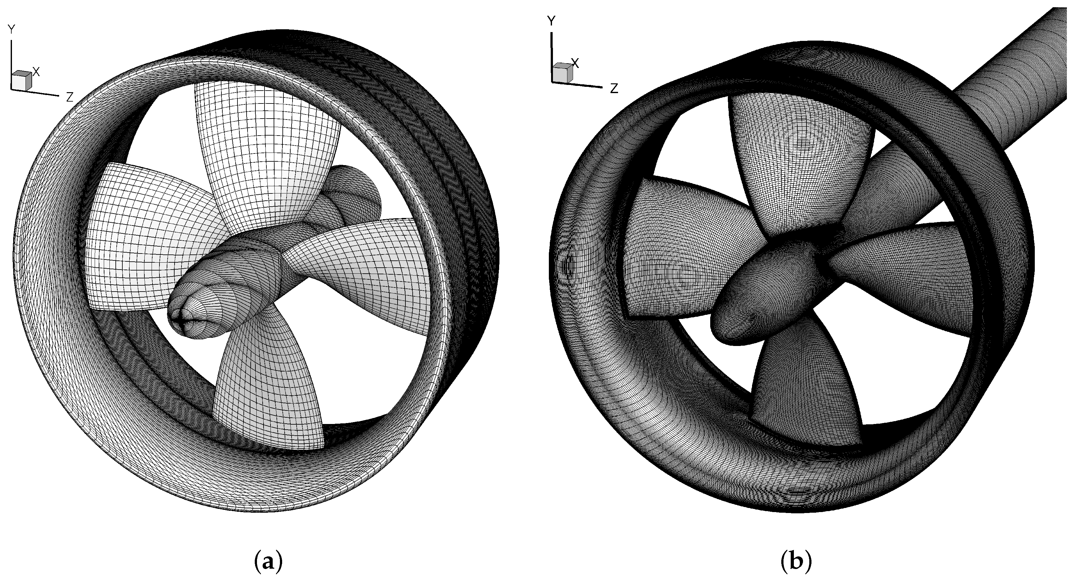
For the RANS simulations, the computational domain is defined as a cylindrical domain with a length of 5 propeller diameters in all directions. For this problem, five nearly-geometrically similar multi-block structured grids were generated using the commercial grid generation package GridPro (www.gridpro.com). The grids range from 1.1 to 26.8 million cells. A fine boundary-layer resolution is considered for all grids, where the maximum dimensionless distance to the wall of the first cell, known as y + , is lower than 1. For the boundary conditions a uniform flow at the inlet and constant pressure at the outer boundary is applied. At the outlet, an outflow condition of zero downstream gradient is used. For the propeller blades, duct and hub, a non-slip boundary condition is set. A rotational velocity is prescribed to the blades and hub, while the duct does not rotate.
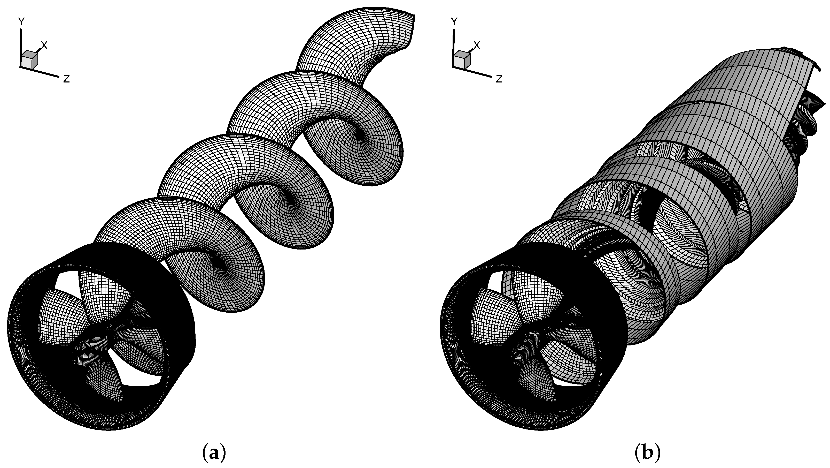
In Figure 4 an overview of the grids used for the calculations with panel code PROPAN and RANS code ReFRESCO is shown.
The variation in thrust and torque for the different grid sizes is listed in Table 2 at J = 0.5 . A reduction in the variation of the open-water quantities with the increased number of cells is observed. Although the differences are less than 1% for the grid with 12.9 million cells, the finest grid (26.8 million cells) is used in the comparative study, since not only the propeller forces, but also local flow quantities are considered in the present analysis. For the prediction of the open-water performance, the ducted propeller is tested for a range of advance coefficients between 0.0 and 0.8 corresponding to Reynolds numbers from 3.5 × 10 5 to 3.8 × 10 5 , where the Reynolds number is defined based on the propeller blade chord length at 0.7 R and the resulting onset velocity at that radius.

3.2. Influence of the Wake Model

In this section the influence of the wake model is studied. The analysis is presented for three advance coefficients: 0.1 , 0.2 and 0.5 . The advance coefficients 0.1 and 0.2 refer to highly loaded conditions from where significant differences are still obtained with the present inviscid model, see Baltazar et al. [11,13].
The inviscid thrust and torque coefficients are compared with experimental open-water data in Table 3. Significant differences are seen in the propeller thrust and torque at low advance coefficients with the rigid wake model. By using the wake alignment model, which includes a correction in the axial velocity due to the interaction between the blade wake and the duct boundary-layer, a reduction in the propeller force coefficients is obtained and lower differences in comparison with the experimental data are observed. This effect has been studied before [11] and is related to the local reduction of the blade wake pitch near the tip which is responsible for lower incidence angles to the blade sections and as a consequence lower propeller forces. Figure 5 presents the blade wake geometries obtained with the rigid wake model (a) and wake alignment model (b) for J = 0.2 . As we can see from Figure 5 the correction in the axial velocity due to the duct boundary-layer introduces a significant reduction in the vortex pitch at the blade wake tip.
Still, an over-prediction of the propeller forces is obtained with the panel method (
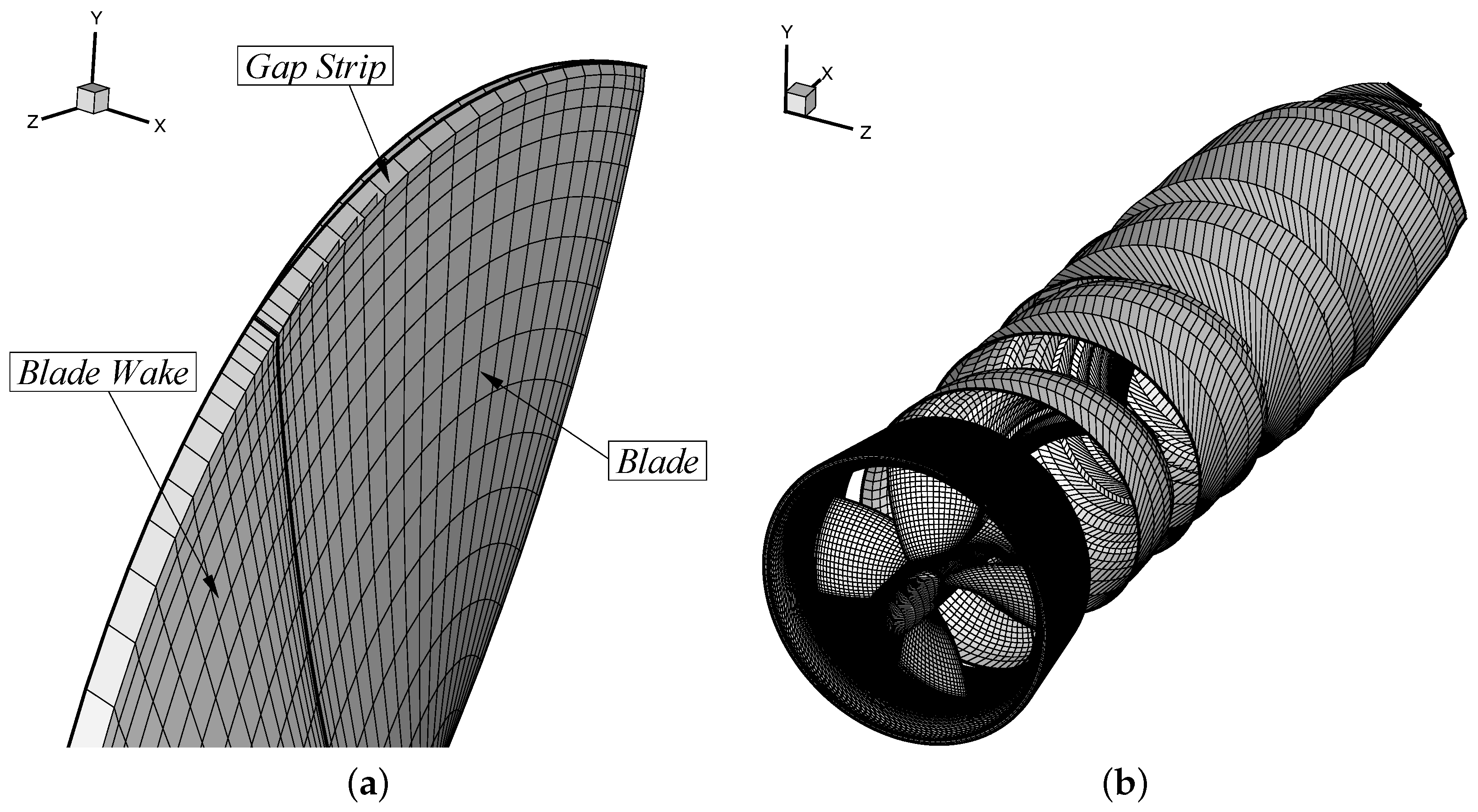
Table 3). These differences suggest that larger corrections to the blade wake pitch are needed and a new wake model is considered, where the gap strip is rotated from the leading edge to reduce its pitch. In this study, the pitch of the gap strip is assumed to be equal to P / D = 0.9 , whereas the blade pitch is constant and equal to P / D = 1.0 . In Figure 6a detail of the gap strip and the obtained blade wake geometry are shown. We note that the gap strip is modelled as a rigid surface and is disconnected from the wake alignment model. The blade wake pitch near the tip may be controlled by the duct boundary-layer correction, Equation (6). However, for low advance ratios large corrections are needed and this has led to divergence of the Kutta condition and non-smooth surface grids. Therefore, the reduction of the gap strip pitch has proven to be a robust technique and can be applied at low advance ratios. As expected, a higher reduction in the propeller thrust and torque is obtained with the wake alignment model using a reduced pitch for the gap strip and approaches the results of the experimental data, see 
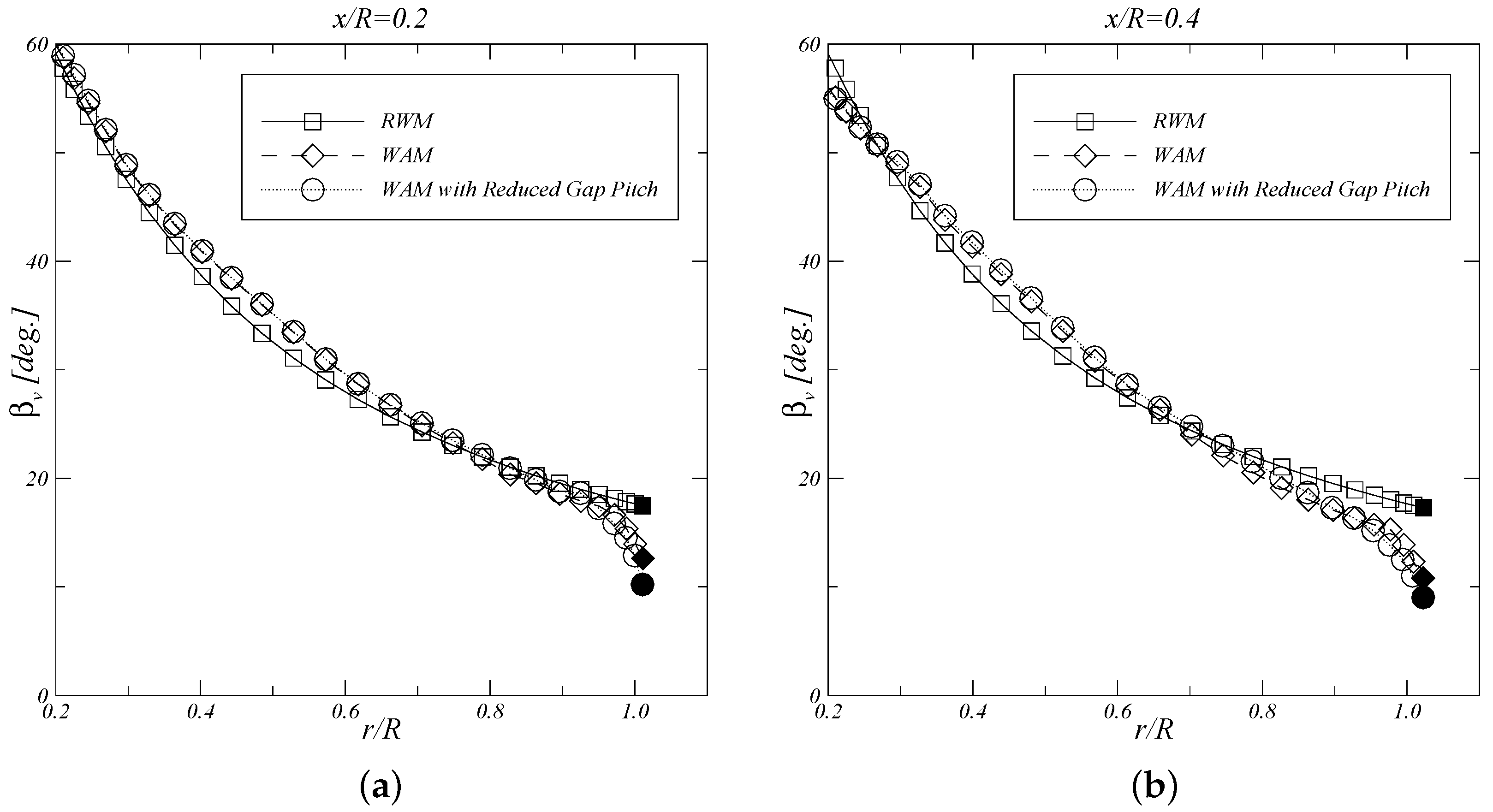
Table 3. The pitch angle of the blade wake β v at the axial positions x / R = 0.2 and 0.4 downstream from the propeller is illustrated in Figure 7, where the local reduction of the wake pitch near the tip is visible.

3.3. Comparison Between PROPAN and ReFRESCO

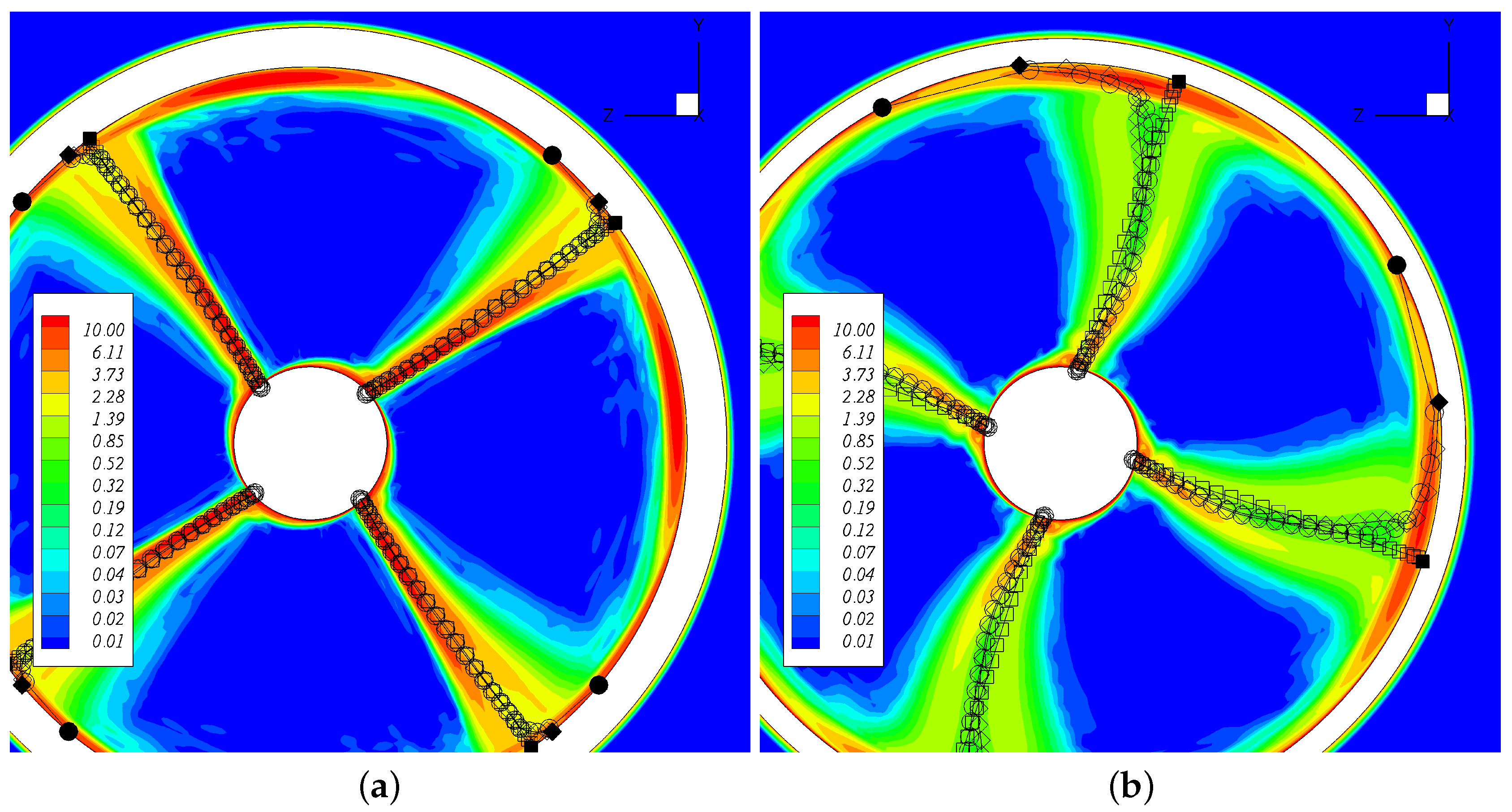
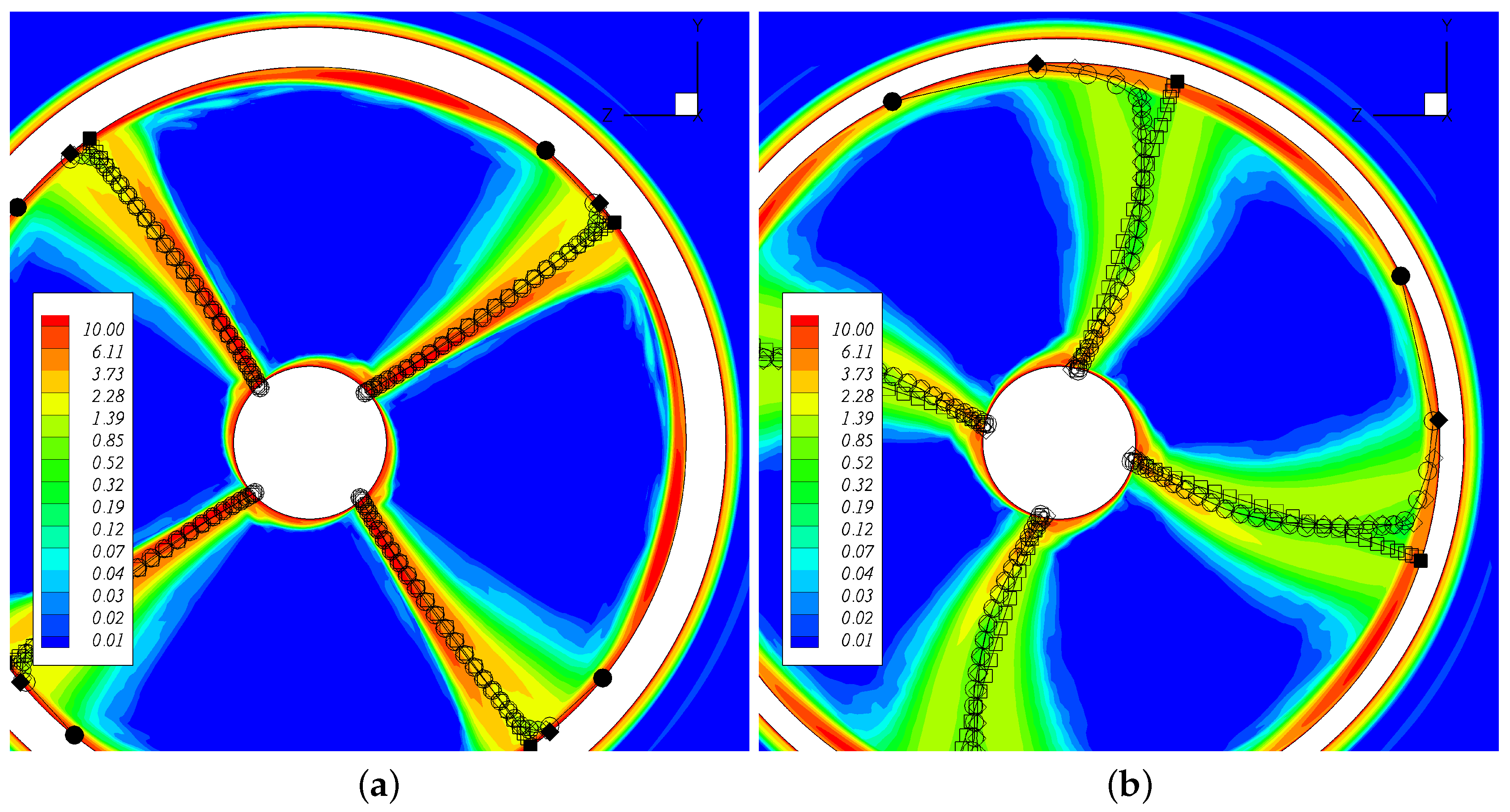
In order to assess on the quality of the inviscid potential model, the results obtained with the panel code PROPAN and RANS code ReFRESCO are compared. The inviscid wake geometry obtained with the three wake models is compared with the vorticity field at the planes x / R = 0.2 and x / R = 0.4 downstream from the propeller, and the blade and duct pressure distributions are shown for the same advance ratios in Figure 8, Figure 9, Figure 10, Figure 11, Figure 12 and Figure 13.
Once again, a reduction in the pitch of the tip vortex is seen when changing from the rigid wake model to the wake alignment model. However, the assessment of the correct location of the tip vortex core from the ReFRESCO calculations is difficult to make due to the interaction between the tip vortex and the duct boundary-layer, creating a viscous flow region at the duct inner side.
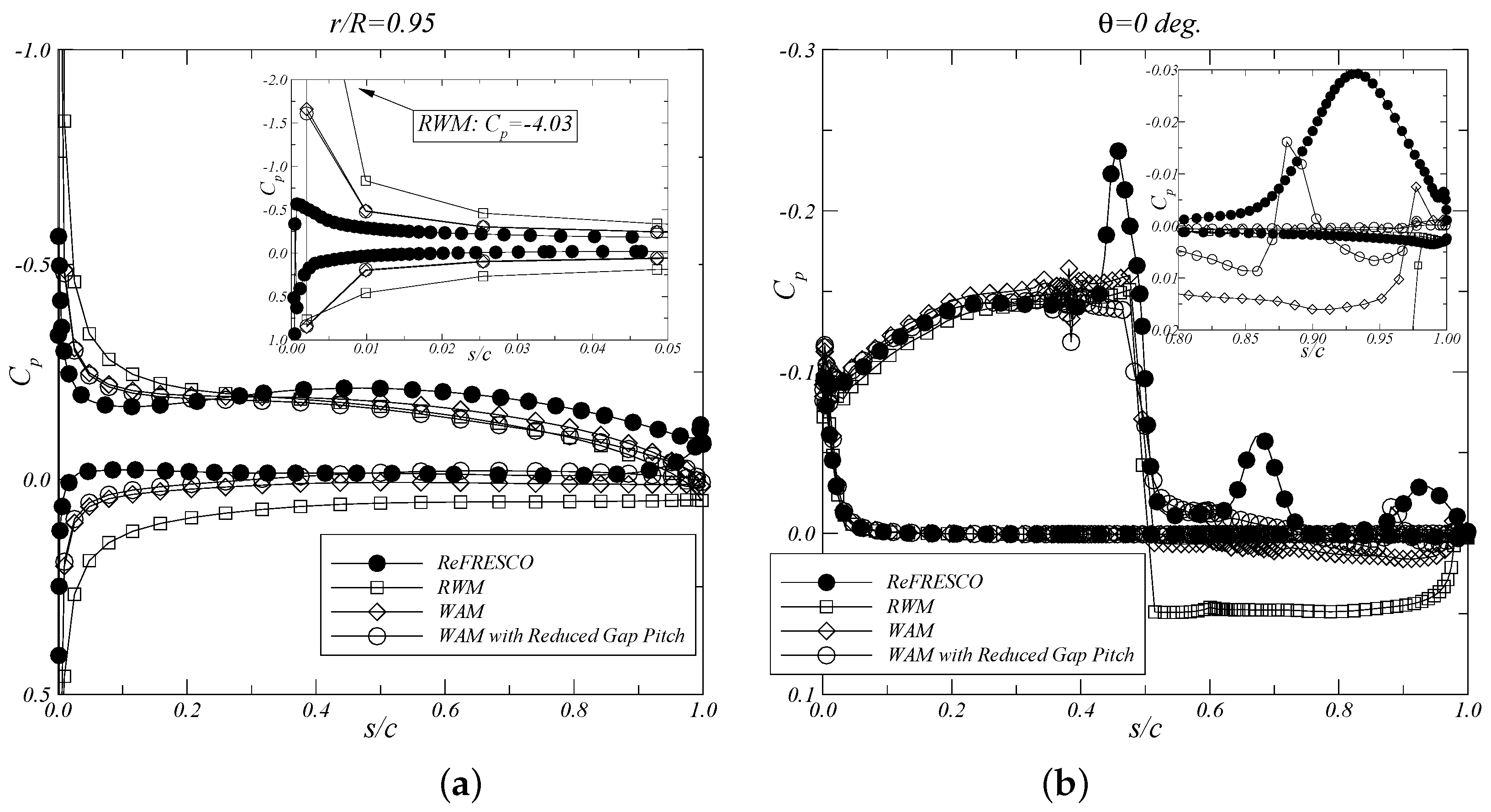
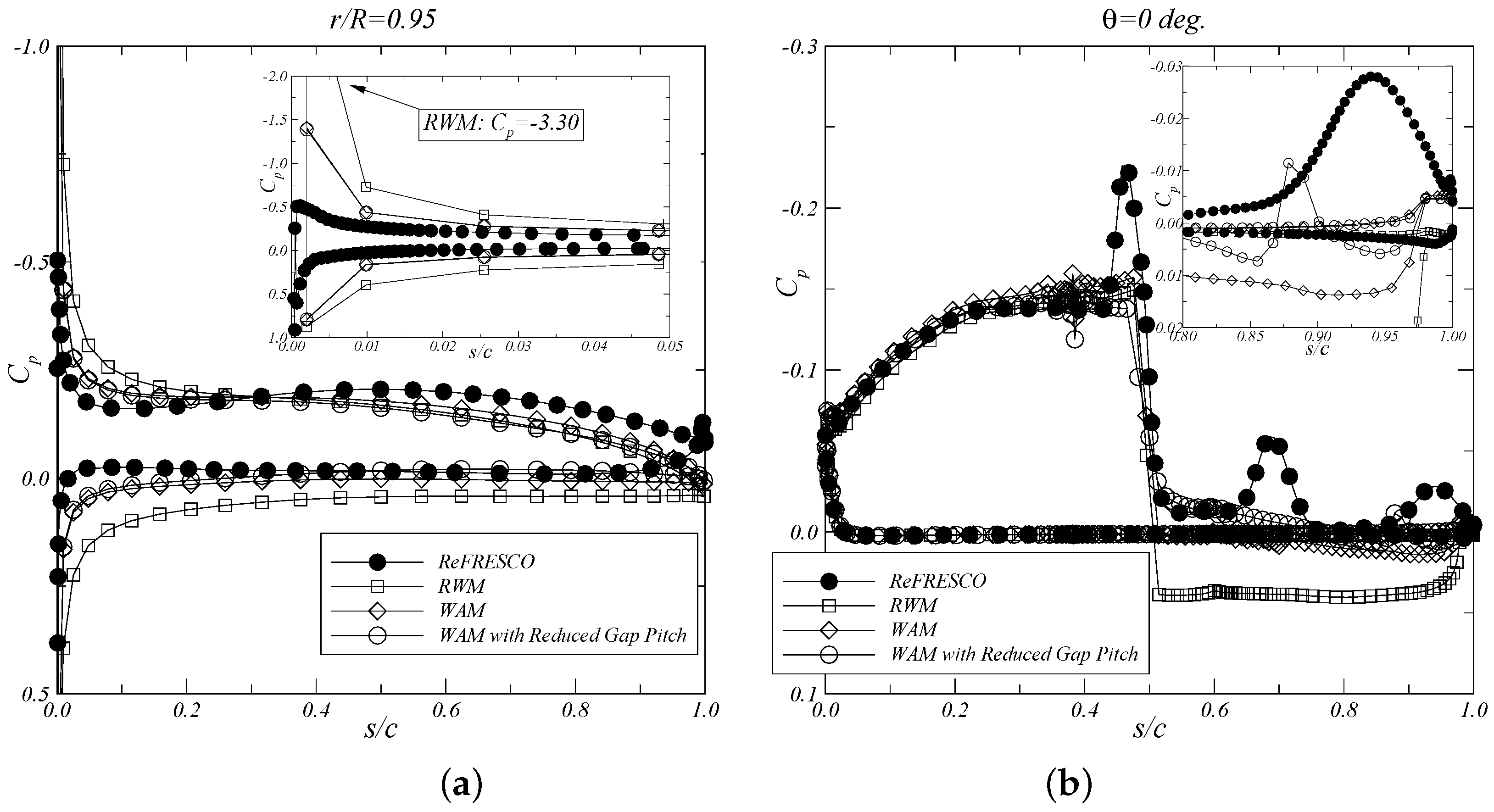
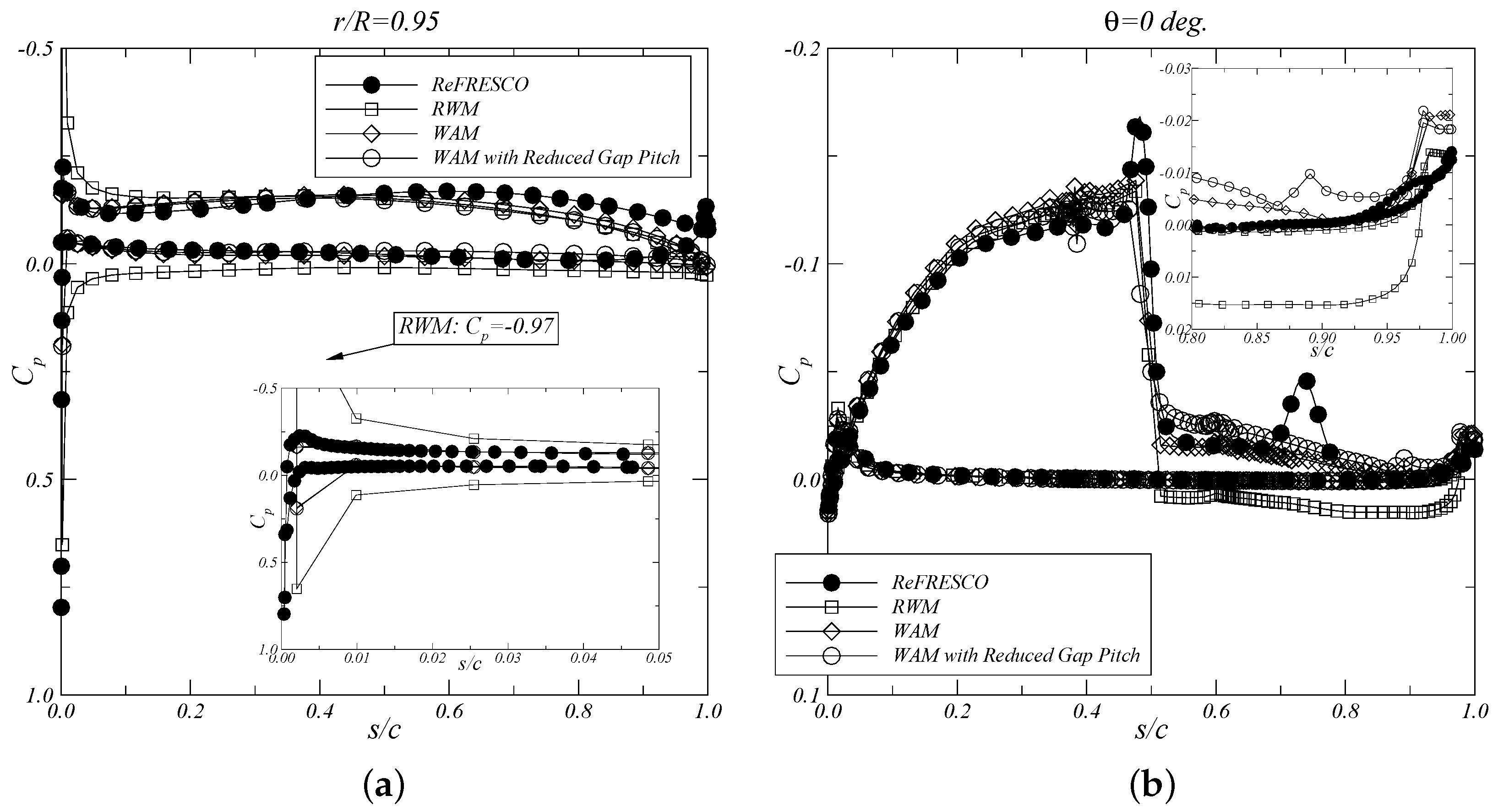
The comparison of the blade and duct pressure distributions is presented along the chordwise direction s / c at the radial section r / R = 0.95 and circumferential position θ = 0 degrees, respectively. For the advance ratios 0.1 and 0.2 , an improvement in the agreement between the inviscid and viscous pressure distributions is obtained when using the wake alignment model with reduced pitch for the gap strip. This comparison shows the influence of the tip vortex pitch on the prediction of the pressure distribution, especially on the duct inner side downstream of the propeller. A decrease in the duct pressure downstream of the propeller is obtained with the reduction of the tip vortex pitch, which is consistent with the viscous results. A reduction in the suction peak at the blade leading edge is also visible, since the blade wake sheet strongly affects the local flow direction to the blade sections. For the pressure distribution at J = 0.5 , a good agreement in the blade suction peak and duct pressure distribution downstream from the propeller is achieved with the wake alignment model. In this case, no significant improvements are obtained when combining the wake alignment model with the reduced gap pitch. For this advance coefficient, the assumption of a duct thickness equal to δ / R = 4 % is sufficient for the correct prediction of the propeller and duct loads.
However, from this study two exceptions are observed in the comparison of the pressure distributions: at the blade leading edge near the tip and in the duct inner side. For the blade pressure, a larger suction peak is obtained with the inviscid model. This suction peak decreases with the reduction of the blade wake pitch at the tip. For the duct pressure at the inner side, local pressure minima are observed in the viscous computations, which are related to the passage of the tip vortices from the different blades. This effect is not captured by the inviscid calculations due to the closed gap model, where the blade wake is attached to the duct inner side.
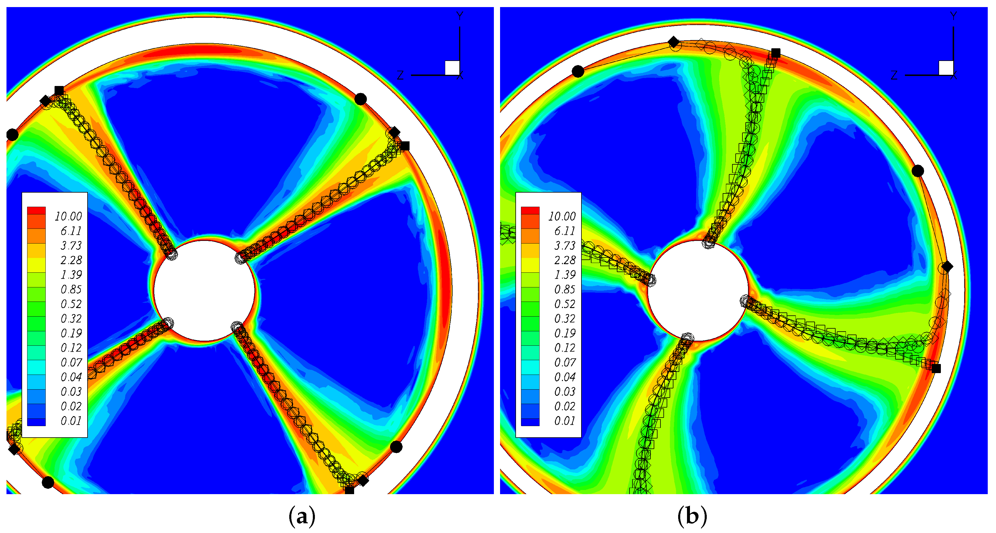
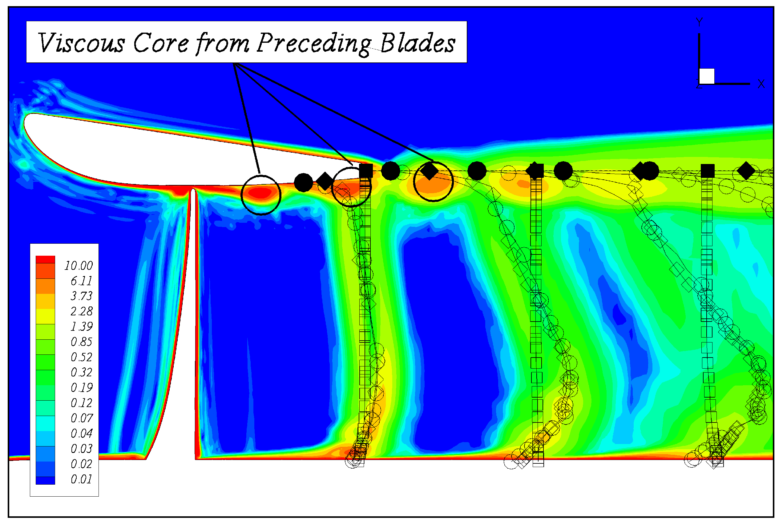
The correlation between the position of the tip vortex core and the peaks of low pressure is illustrated in Figure 14 for the plane z = 0 at J = 0.2 , which corresponds to the circumferential position θ = 0 degrees. In this figure the inviscid wake geometries are compared with the viscous total vorticity field along the longitudinal direction. A good agreement is obtained with the aligned wakes, except near the blade wake tip, where some differences are still observed.

3.4. Prediction of the Open-Water Performance

In this section the predicted thrust and torque coefficients are compared with experimental data available from open-water tests [23]. In the wake alignment model the duct boundary-layer thickness ( δ / R = 4 % ) is assumed independent of the inflow conditions for the entire open-water range. In addition, in the wake alignment model with reduced gap pitch a constant value of P / D = 0.9 is also considered for all advance coefficients. The ReFRESCO calculations are also included in the comparison. 
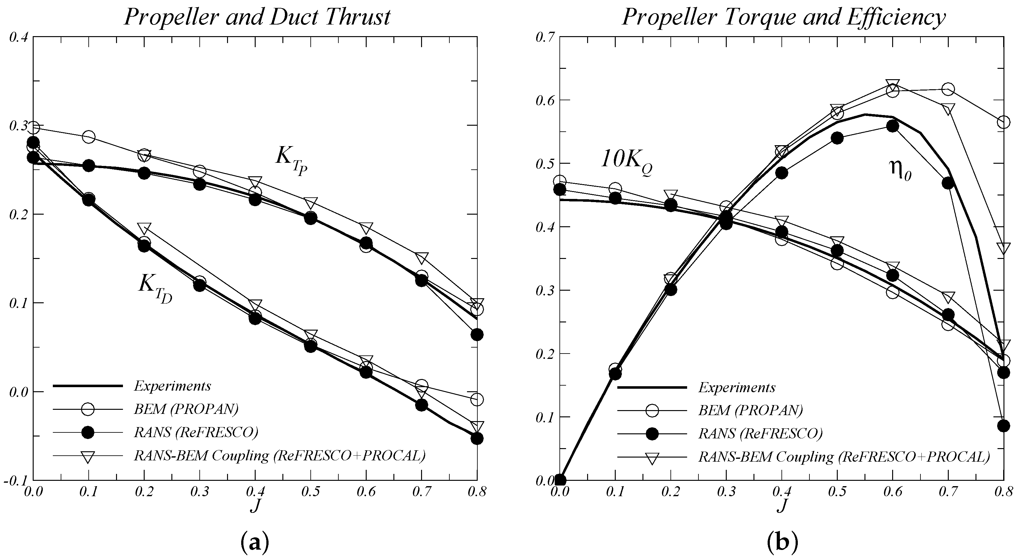
Figure 15 illustrates the comparison of the thrust and torque coefficients with the experiments. A section viscous drag coefficient of 0.007 and suppression of the chordwise component of the blade section lift are considered for all inviscid computations. This suppression models the effect of flow separation which eliminates the non-physical suction peaks at the leading edge in the potential flow theory. No viscous drag correction to the duct thrust has been applied.
As expected, a significant over-prediction of the propeller thrust and torque is obtained with the rigid wake model. This result shows that the prescribed wake geometry with constant pitch and equal to the blade pitch completely misses the propeller and duct loads. Alternatively, the propeller thrust and torque are well predicted for the advance ratios higher than 0.3 when using the wake alignment model without gap pitch correction. For the advance ratios lower than 0.3 a significant improvement in the comparison with the experiments is obtained with the wake alignment model using a reduced pitch for the gap strip.
Although the assumptions of constant duct boundary-layer thickness and gap strip pitch independent of the inflow conditions are questionable, a reasonable to good agreement of the propeller forces is obtained with the wake alignment model when compared with the experiments. For example, at J = 0.1 the differences between the measured and the predicted propeller thrust reduce from 20% to 7% by applying the gap pitch reduction. For the propeller torque, the differences decrease from 12% to 0.3% with the reduced gap pitch. A smaller influence of the gap pitch is observed for the higher advance coefficients, which is due to the decrease of the tip vortex strength. The duct thrust coefficient agrees well with the measurements for low advance coefficients. For high advance coefficients, an over-prediction of the duct thrust is seen, which is due to the occurrence of flow separation on the outer side of the duct and it is not modelled in the inviscid method.
A good agreement of the propeller forces with the experimental data is obtained with the viscous calculations using code ReFRESCO for advance ratios up to 0.7 . In this range the differences are in the order of 1%. This agreement legitimates the use of RANS simulations for the present comparison study.

4. Conclusions

The investigation presented in this paper focused on the improvement of the inviscid performance predictions with a panel method for ducted propellers. For this study, a comparison between the results obtained by a panel method with a RANS solver is made to obtain a better insight on the viscous effects of the ducted propeller and on the limitations of the inviscid potential flow model. Special attention is given near bollard pull conditions, which are important in the design of ducted propeller systems. Results show that an alignment model of the wake geometry with the local flow is essential for an accurate prediction of the propeller and duct loads. Due to the strong interaction between the blade wake and the boundary-layer on the duct inner side, a correction in the axial velocity is also taken into account in the wake alignment model. As a consequence, a local reduction of the blade wake pitch near the tip is obtained influencing the propeller loading. However, this mechanism is not sufficient to correctly predict the propeller forces near bollard pull and an additional correction is proposed for the gap strip. In the present work, the pitch of the gap strip is empirically prescribed in a first attempt to model the tip leakage vortex. In this way, a stronger reduction in the blade wake pitch is obtained and the agreement of the propeller forces with the experiments improves significantly over the entire open-water range. The wake alignment scheme combined with empirical corrections for the blade wake pitch near the tip and gap strip, to take into account the viscous effects of the gap flow in the potential flow model, has proven to be robust, efficient and to provide accurate predictions of the open-water performance of ducted propellers.

Acknowledgments

The authors acknowledge the Laboratory for Advanced Computing at University of Coimbra (www.lca.uc.pt) for providing computing resources that have contributed to part of the results reported in this paper.

Author Contributions

J.M.B. and J.F.C. developed the inviscid panel method with the contribution from J.B. in the implementation of the wake alignment model. D.R. generated the grids and conduct the viscous calculations with the RANS solver. J.M.B. ran the inviscid code, analysed the output data and compared the inviscid and viscous results. J.B. provided scientific advice and supervision throughout. All authors discussed the results and commented on the manuscript.

Conflicts of Interest

The authors declare no conflict of interest.

Abbreviations

The following abbreviations are used in this manuscript:
ISTInstituto Superior Técnico
MARINMaritime Research Institute Netherlands
QUICKQuadratic upwind interpolation for convective kinematics
RANSReynolds-averaged Navier-Stokes
RWMRigid wake model
SIMPLESemi-implicit method for pressure linked equations
SSTShear stress transport
WAMWake alignment model

References

  1. Sánchez-Caja, A.; Rautaheimo, P.; Siikonen, T. Simulation of Incompressible Viscous Flow Around a Ducted Propeller Using a RANS Equation Solver. In Proceedings of the Twenty-Third Symposium on Naval Hydrodynamics, Val de Reuil, France, 17–22 September 2000; The National Academies Press: Washington, DC, USA, 2001; pp. 527–539. [Google Scholar]
  2. Sánchez-Caja, A.; Pylkkänen, J.V.; Sipilä, T.P. Simulation of the Incompressible Viscous Flow Around Ducted Propellers With Rudders Using a RANSE solver. In Proceedings of the 27th Symposium on Naval Hydrodynamics, Seoul, Korea, 5–10 October 2008; Curran Associates, Inc.: Red Hook, NY, USA, 2010; pp. 968–982. [Google Scholar]
  3. Abdel-Maksoud, M.; Heinke, H.-J. Scale Effects on Ducted Propellers. In Proceedings of the Twenty-Fourth Symposium on Naval Hydrodynamics, Fukuoka, Japan, 8–13 July 2002; The National Academies Press: Washington, DC, USA, 2003; pp. 744–759. [Google Scholar]
  4. Bhattacharyya, A.; Krasilnikov, V.; Steen, S. Scale effects on open water characteristics of a controllable pitch propeller working within different duct designs. Ocean Eng. 2016, 112, 226–242. [Google Scholar] [CrossRef]
  5. Kim, J.; Paterson, E.G.; Stern, F. RANS simulation of ducted marine propulsor flow including subvisual cavitation and acoustic modeling. ASME J. Fluids Eng. 2006, 128, 799–810. [Google Scholar] [CrossRef]
  6. Kerwin, J.E.; Kinnas, S.A.; Lee, J.-T.; Shih, W.-Z. A Surface Panel Method for the Hydrodynamic Analysis of Ducted Propellers. In Transactions of Society of Naval Architects and Marine Engineers; Society of Naval Architects and Marine Engineers: New York, NY, USA, 1987; p. 4. [Google Scholar]
  7. Hughes, M.J.; Kinnas, S.A.; Kerwin, J.E. Experimental validation of a ducted propeller analysis method. ASME J. Fluids Eng. 1992, 114, 214–219. [Google Scholar] [CrossRef]
  8. Hughes, M.J. Implementation of a Special Procedure for Modeling the Tip Clearance Flow in a Panel Method for Ducted Propulsors. In Proceedings of the Propellers & Shafting ’97 Symposium, Virginia Beach, VA, USA, 23–24 September 1997; Society Naval Architects and Marine Engineers: Alexandria, VA, USA, 1997. Paper Number 17. [Google Scholar]
  9. Lee, H.; Kinnas, S.A. Prediction of Cavitating Performance of Ducted Propellers. In Proceedings of the Sixth International Symposium on Cavitation, Wageningen, The Netherlands, 11–15 September 2006. [Google Scholar]
  10. Oweis, G.F.; Fry, D.; Jessup, S.D.; Ceccio, S.L. Development of a tip-leakage flow—Part 1: The flow over a range of Reynolds numbers. ASME J. Fluid Eng. 2006, 128, 751–764. [Google Scholar] [CrossRef]
  11. Baltazar, J.; Falcão de Campos, J.A.C.; Bosschers, J. Open-water thrust and torque predictions of a ducted propeller system with a panel method. Int. J. Rotating Mach. 2012, 2012, 474785. Available online: https://www.hindawi.com/journals/ijrm/2012/474785/ (accessed on 16 January 2018). [CrossRef]
  12. Baltazar, J.; Rijpkema, D.; Falcão de Campos, J.A.C. A Comparison of Panel Method and RANS Calculations for a Ducted Propeller System in Open-Water. In Proceedings of the Third International Symposium on Marine Propulsors, Launceston, Australia, 5–8 May 2013; Binns, J., Brown, R., Bose, N., Eds.; Australian Maritime College, University of Tasmania: Newnham, TAS, Australia, 2013; pp. 338–346. [Google Scholar]
  13. Baltazar, J.; Falcão de Campos, J.A.C.; Bosschers, J. Potential Flow Modelling of Ducted Propellers with a Panel Method. In Proceedings of the Fourth International Symposium on Marine Propulsors, Austin, TX, USA, 31 May–4 June 2015; Kinnas, S.A., Ed.; The University of Texas at Austin: Austin, TX, USA, 2015; pp. 184–192. [Google Scholar]
  14. Vaz, G.; Bosschers, J. Modelling Three Dimensional Sheet Cavitation on Marine Propellers Using a Boundary Element Method. In Proceedings of the Sixth International Symposium on Cavitation, Wageningen, The Netherlands, 11–15 September 2006. [Google Scholar]
  15. Bosschers, J.; Willemsen, C.; Peddle, A.; Rijpkema, D. Analysis of Ducted Propellers by Combining Potential Flow and RANS Methods. In Proceedings of the Fourth International Symposium on Marine Propulsors, Austin, TX, USA, 31 May–4 June 2015; Kinnas, S.A., Ed.; The University of Texas at Austin: Austin, TX, USA, 2015; pp. 639–648. [Google Scholar]
  16. Gu, H.; Kinnas, S.A. Modeling of Contra-Rotating and Ducted Propellers via Coupling of a Vortex-Lattice with a Finite Volume Method. In Proceedings of the Propellers & Shafting 2003 Symposium, Virginia Beach, VA, USA, 17–18 September 2003; Society Naval Architects and Marine Engineers: Alexandria, VA, USA, 2003. [Google Scholar]
  17. Kinnas, S.A.; Fan, H.; Tian, Y. A Panel Method with a Full Wake Alignment Model for the Prediction of the Performance of Ducted Propellers. J. Ship Res. 2015, 59, 246–257. [Google Scholar] [CrossRef]
  18. Kim, S.; Du, W.; Kinnas, S.A. Panel Method for Ducted Propellers with Sharp and Round Trailing Edge Duct With Fully Aligned Wake on Blade and Duct. In Proceedings of the Fifth International Symposium on Marine Propulsors, Espoo, Finland, 12–15 June 2017; Sánchez-Caja, A., Ed.; VTT Technical Research Center of Finland Ltd.: Espoo, Finland, 2017; pp. 627–636. [Google Scholar]
  19. Baltazar, J. On the Modelling of the Potential Flow About Wings and Marine Propellers Using a Boundary Element Method. Ph.D. Thesis, Instituto Superior Técnico, Lisbon, Portugal, 30 September 2008. [Google Scholar]
  20. Morino, L.; Kuo, C.-C. Subsonic potential aerodynamics for complex configurations: A general theory. AIAA J. 1974, 12, 191–197. [Google Scholar]
  21. Vaz, G.; Jaouen, F.; Hoekstra, M. Free-Surface Viscous Flow Computations. Validation of URANS Code FreSCo. In Proceedings of the ASME 28th International Conference on Ocean, Offshore and Arctic Engineering, OMAE2009-79398, Honolulu, HI, USA, 31 May–5 June 2009; pp. 425–437. [Google Scholar]
  22. Menter, F.; Kuntz, M.; Langtry, R. Ten Years of Industrial Experience With the SST Turbulence Model. In Proceedings of the Fourth International Symposium on Turbulence, Heat and Mass Transfer, Antalya, Turkey, 12–17 October 2003; Hanjalić, K., Nagano, Y., Tummers, M.J., Eds.; Begell House: Danbury, CT, USA, 2003; pp. 625–632. [Google Scholar]
  23. Kuiper, G. The Wageningen Propeller Series; Maritime Research Institute Netherlands: Wageningen, The Netherlands, 1992; ISBN 9090072470. [Google Scholar]
Figure 1. Schematic overview of the flow in the gap region between blade tip and duct inner side.
Jmse 06 00027 g001
Figure 2. Propeller coordinate systems.
Jmse 06 00027 g002
Figure 3. Pressure Kutta condition for the duct trailing edge with a thick round geometry and L denoting the duct length.
Jmse 06 00027 g003
Figure 4. Overview of the surface grids used for the inviscid calculations with PROPAN (a) and RANS calculations with ReFRESCO (b).
Jmse 06 00027 g004
Figure 5. Panel arrangement for propeller blades, duct, hub and blade wake at J = 0.2 . Rigid wake model (a); Wake alignment model (b). Only one wake surface is shown.
Jmse 06 00027 g005
Figure 6. Wake alignment model with reduced gap pitch of P / D = 0.9 . Detail of the gap strip and blade wake sheet (a); Overview of one blade wake geometry for J = 0.2 (b).
Jmse 06 00027 g006
Figure 7. Vortex pitch β v distribution at x / R = 0.2 (a) and x / R = 0.4 (b) for J = 0.2 . Influence of the wake model. The filled symbols refer to the tip vortex.
Jmse 06 00027 g007
Figure 8. Wake geometry at x / R = 0.2 (a) and x / R = 0.4 (b) for J = 0.1 . The contours represent the ReFRESCO total vorticity field | ω | / Ω . The symbols represent the PROPAN wake geometry: rigid wake model (squares), wake alignment model (diamonds) and wake alignment model with reduced gap pitch (circles). The filled symbols refer to the tip vortex.
Jmse 06 00027 g008
Figure 9. Blade chordwise pressure distribution at r / R = 0.95 (a); Duct chordwise pressure distribution at θ = 0 degrees (b). J = 0.1 .
Jmse 06 00027 g009
Figure 10. Wake geometry at x / R = 0.2 (a) and x / R = 0.4 (b) for J = 0.2 . The contours represent the ReFRESCO total vorticity field | ω | / Ω . The symbols represent the PROPAN wake geometry: rigid wake model (squares), wake alignment model (diamonds) and wake alignment model with reduced gap pitch (circles). The filled symbols refer to the tip vortex.
Jmse 06 00027 g010
Figure 11. Blade chordwise pressure distribution at r / R = 0.95 (a); Duct chordwise pressure distribution at θ = 0 degrees (b). J = 0.2 .
Jmse 06 00027 g011
Figure 12. Wake geometry at x / R = 0.2 (a) and x / R = 0.4 (b) for J = 0.5 . The contours represent the ReFRESCO total vorticity field | ω | / Ω . The symbols represent the PROPAN wake geometry: rigid wake model (squares), wake alignment model (diamonds) and wake alignment model with reduced gap pitch (circles). The filled symbols refer to the tip vortex.
Jmse 06 00027 g012
Figure 13. Blade chordwise pressure distribution at r / R = 0.95 (a); Duct chordwise pressure distribution at θ = 0 degrees (b). J = 0.5 .
Jmse 06 00027 g013
Figure 14. Wake geometry at z = 0 for J = 0.2 . The contours represent the ReFRESCO total vorticity field | ω | / Ω . The symbols represent the PROPAN wake geometry: rigid wake model (squares), wake alignment model (diamonds) and wake alignment model with reduced gap pitch (circles). The filled symbols refer to the tip vortex.
Jmse 06 00027 g014
Figure 15. Comparison between numerical and experimental data from open-water tests. Propeller and duct thrust (a); Propeller torque and open-water efficiency (b).
Jmse 06 00027 g015
Table 1. Variation of open-water characteristics with different grid sizes compared to the finest grid. Panel method computations at J = 0.5 .
Grid Size (Blade + Duct + Hub) 1 Δ K T P Δ K T D Δ K Q
20 × 11 + 100 × 40 + 39 × 32−4.76%−7.42%−5.97%
30 × 16 + 130 × 80 + 51 × 48−0.60%−3.34%−1.42%
40 × 21 + 160 × 120 + 63 × 64−0.79%−1.30%−1.23%
50 × 26 + 190 × 160 + 75 × 80−0.49%−0.37%−0.74%
60 × 31 + 220 × 200 + 87 × 96−0.15%−0.19%−0.25%
70 × 36 + 250 × 240 + 98 × 112
1 The grid size refers to the chordwise and spanwise radial directions for each propeller blade, and to the streamwise and circumferential directions for the duct and hub.
Table 2. Variation of open-water characteristics with different grid sizes compared to the finest grid with M denoting million. RANS computations at J = 0.5 .
Grid Size Δ K T P Δ K T D Δ K Q
1.1 M3.25%2.39%3.55%
2.6 M2.78%2.78%2.75%
7.7 M0.67%1.99%0.69%
12.9 M0.21%0.99%0.28%
26.8 M
Table 3. Inviscid thrust and torque coefficients for J = 0.1 , 0.2 and 0.5 and comparison with experimental data [23]. Influence of the wake model.
Model K T P K T D 10 K Q
J = 0.1
RWM0.4120.2060.5882
WAM0.3130.2310.4664
WAM with Reduced Gap Pitch0.2840.2260.4228
Experiments0.2540.2140.4387
J = 0.2
RWM0.3830.1600.5538
WAM0.2970.1760.4456
WAM with Reduced Gap Pitch0.2730.1710.4083
Experiments0.2480.1660.4279
J = 0.5
RWM0.2660.0540.4041
WAM0.2080.0570.3246
WAM with Reduced Gap Pitch0.1930.0550.3010
Experiments0.1960.0530.3506

